Randomized maximum likelihood based posterior sampling
←
→
Page content transcription
If your browser does not render page correctly, please read the page content below
Noname manuscript No.
                                           (will be inserted by the editor)

                                           Randomized maximum likelihood based posterior
                                           sampling

                                           Yuming Ba · Jana de Wiljes · Dean S.
                                           Oliver · Sebastian Reich
arXiv:2101.03612v2 [math.NA] 17 Aug 2021

                                           Received: date / Accepted: date

                                           Abstract Minimization of a stochastic cost function is commonly used for ap-
                                           proximate sampling in high-dimensional Bayesian inverse problems with Gaus-
                                           sian prior distributions and multimodal posterior distributions. The density of
                                           the samples generated by minimization is not the desired target density, unless
                                           the observation operator is linear, but the distribution of samples is useful as
                                           a proposal density for importance sampling or for Markov chain Monte Carlo
                                           methods. In this paper, we focus on applications to sampling from multimodal
                                           posterior distributions in high dimensions. We first show that sampling from
                                           multimodal distributions is improved by computing all critical points instead of
                                           only minimizers of the objective function. For applications to high-dimensional
                                           geoscience inverse problems, we demonstrate an efficient approximate weight-
                                           ing that uses a low-rank Gauss-Newton approximation of the determinant of
                                           the Jacobian. The method is applied to two toy problems with known posterior
                                           distributions and a Darcy flow problem with multiple modes in the posterior.

                                           Yuming Ba
                                           School of Mathematics, Hunan University, Changsha 410082, China
                                           E-mail: yumingb9630@163.com
                                           Present address: School of Mathematics and Systems Science, Guangdong Polytechnic Nor-
                                           mal University, Guangzhou 510665
                                           Jana de Wiljes
                                           Universität Potsdam, Institut für Mathematik, Karl-Liebknecht-Str. 24/25, D-14476 Pots-
                                           dam, Germany
                                           E-mail: wiljes@uni-potsdam.de
                                           Dean S. Oliver
                                           NORCE Norwegian Research Centre, Bergen, Norway
                                           E-mail: dean.oliver@norceresearch.no
                                           Sebastian Reich
                                           Universität Potsdam, Institut für Mathematik, Karl-Liebknecht-Str. 24/25, D-14476 Pots-
                                           dam, Germany
                                           E-mail: sebastian.reich@uni-potsdam.de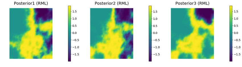
2                                       Y. Ba, J. de Wiljes, D. S. Oliver and S. Reich

Keywords Randomized maximum likelihood · Importance sampling ·
Minimization · Multimodal posterior · Bayesian inverse problem

1 Introduction

In several fields, including groundwater management, groundwater remedia-
tion, and petroleum reservoir management, there is a need to characterize
permeable rock bodies whose properties are spatially variable. In most cases,
the reservoirs are deeply buried, the number of parameters needed to charac-
terize the porous medium is large and the observations are sparse and indirect
[33]. In these applications, the problem of estimating model parameters is al-
most always underdetermined and the desired solution is not simply a best
estimate, but rather a probability density on model parameters conditioned to
the observations and to the prior knowledge [39]. Because the model dimension
in geoscience applications is always large, the posterior distribution is often
represented empirically by samples from the posterior distribution.
    Unfortunately, the posterior probability density for reservoir properties,
conditional to rate and pressure observations, is typically complex and not
easily sampled. Several authors have shown that the log-posterior for subsur-
face flow problems is not convex in some situations [46, 40, 34] so that Gaussian
approximations of the posterior distribution appear to be dangerous. Markov
chain Monte Carlo methods (MCMC) are often considered to provide the gold
standard for sampling from the posterior. It is frequently suggested to be the
method against which other methods are compared [23], yet it can be difficult
to design efficient transition kernels [13, 11] and convergence of MCMC can be
difficult to assess [17]. The number of likelihood function evaluations required
to obtain a modest number of independent samples may be excessive for highly
nonlinear flow problems [35].
    Importance sampling methods can also be considered to be exact sam-
pling methods as they implement Bayes rule directly. They are very difficult
to apply in high dimensions, however, as an efficient implementation requires a
proposal density that is a good approximation of the posterior [5, 28]. Various
methods have been developed in the data assimilation community to ensure
that particles are located in regions of high probability density [24]. Although
not introduced as importance sampling approaches, a variety of methods based
on minimization of a stochastic objective function have been developed, begin-
ning with Kitanidis [21] and Oliver et al. [36] who introduced minimization of
a stochastic objective function as a way of simulating samples from an approx-
imation of the posterior when the prior distribution is Gaussian and the errors
in observations are Gaussian and additive. The distribution of samples based
on minimizers of the objective function was shown to be correct for Gauss-
linear problems, but when the observation operator g(m) is nonlinear, it was
necessary to weight the samples because the sampling was only approximate
in that case.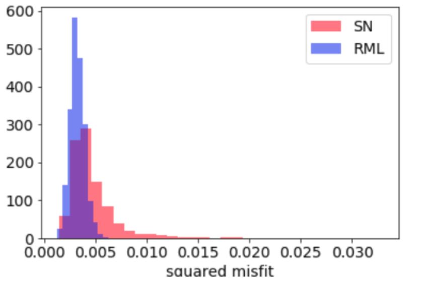
RML based posterior sampling                                                    3

    The randomized maximum likelihood (RML) method approach to sam-
pling has been used without weighting in high dimensional inverse problems
with Gaussian priors [16, 14, 9, 7]. Weights are seldom computed for several rea-
sons: computation of exact weights is infeasible in large dimensions because
the computation of weights requires the second derivative of the observation
operator, the proposal density does not always cover the target density, and
sampling without weighting sometimes provides a good approximation of the
posterior even in posterior distributions with many modes [32]. In practice,
the most popular implementations are the ensemble-Kalman based forms of
the RML method [10, 38, 45, 20] in which a single average sensitivity is used
for minimization so that weighting of samples is not possible.
    Bardsley et al. [3] proposed another minimization-based sampling method-
ology, randomize-then optimize (RTO), in which the need for computation of
the second derivative of the observation operator is avoided for weighting. The
RTO method has then been modified to allow application in very high dimen-
sions [4], but the method is restricted to posterior distributions with a single
mode. Wang et al. [44] discussed the relationship between the cost function in
the RML method and the cost function in the RTO method, and showed that
the methods are equivalent for linear observation operators. Wang et al. also
showed that some approximations to the weights in RML could be computed
in high dimensions and provided a useful comparison of sampling distributions.
    For nonconvex log-posteriors, there could be many (local) minimizers of
the RML and RTO cost functions. Oliver et al. [36] and Oliver [32] suggested
that only the global minimizer should be used for sampling, although finding
the global minimizer would be difficult to ensure. To improve the likelihood
of converging to the global minimizer, they suggested using the unconditional
sample from the prior as the starting point for minimization. In contrast, Wang
et al. [44] investigated the effect of various strategies for choosing the initial
guess on sample distribution and found that a random initial guess worked
well.
    Unlike previous methods that compute minimizers only, we show that exact
sampling is possible when all critical points of a stochastic objective function
are computed and properly weighted. Computing the weights accurately, how-
ever, for all critical points in high dimensions does not appear to be feasible,
but we demonstrate that Gauss-Newton approximations of the weights provide
good approximations for minimizers of the objective function in problems with
multimodal posteriors. The Gauss-Newton approximations of weights can be
obtained as by-products of Gauss-Newton minimization of the objective func-
tion, or as low-rank approximations using stochastic sampling approaches. We
also show that valid sampling can be performed without computing all critical
points, but by instead randomly sampling of the critical points.
    We investigated the performance of both exact sampling and approximate
sampling on two small toy problems for which the sampled distribution can be
compared with the exact posterior probability density. For a problem with two
modes in the posterior pdf, the distribution of samples from weighted RML
using all critical points appears to be correct. Approximate sampling using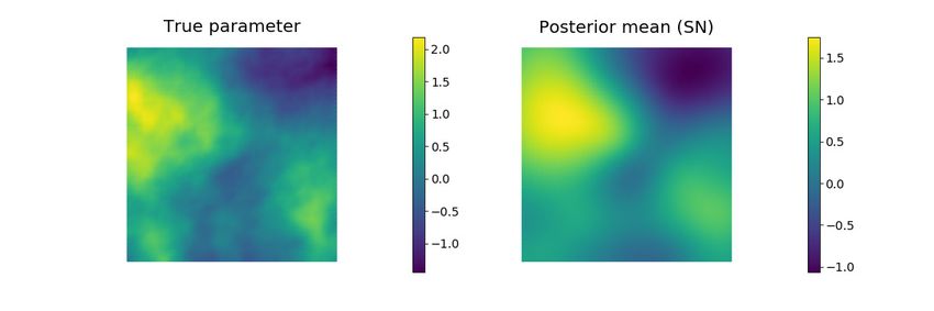
4                                        Y. Ba, J. de Wiljes, D. S. Oliver and S. Reich

Gauss-Newton approximation of weights and minimizers samples well from
both modes, but under-samples the region between modes. The data misfit is
not a useful approximation of the weights in this case.
    We also applied the approximate sampling method to the problem of esti-
mating permeability in a 2D porous medium from 25 measurements of pres-
sure. In this case, the distribution of weights was relatively large, even when
the log-permeability was distributed as multivariate normal. High-dimensional
state spaces such as considered here have a severe effect on importance sam-
pling and remedies such as tempering are suggested to reduce the impact of
the dimensionality on the estimation [6].

2 RML sampling algorithm

Given a prior Gaussian distribution N(m̄, CM ) on a set of model parameters
m ∈ RNm and observations do ∈ RNd which are related to the model param-
eters through a forward map g : RNm → RNd for unknown m∗ and unknown
measurement errors  ∼ N(0, CD ), i.e.,
                                  do = g(m∗ ) + ,                                 (1)
we wish to generate samples mi , i = 1, . . . , Ne , from the posterior distribution

                                 πM D (m, do )
                   πM (m|do ) =                ∝ exp(−L(m))                 (2)
                                    πD (do )
with negative log likelihood function
            1          T   −1            1            T   −1
   L(m) = (m − m̄) CM         (m − m̄) + (g(m) − do ) CD     (g(m) − do ) . (3)
            2                            2
The normalisation constant πD (do ) is unknown, in general. We will use πM (m) :=
πM (m|do ) in order to simplify notation.
    In this paper, we will show how to use the RML method in order to produce
independent weighted Monte Carlo samples from the posterior distribution (2).
Posterior sampling problems of the form (2) with negative log likelihood func-
tion (3) arise from many practical Bayesian inference problems. In practical
applications, where the number of model parameters is typically large, the
computation of exact weights is infeasible. For those cases we suggest approx-
imations.

2.1 The trial distribution: RML as proposal step

The RML method draws samples (m0i , δi0 ), i = 1, . . . , Ns , from the Gaussian
distribution
                                         1
    qM 0 ∆0 (m0 , δ 0 ) =      N  N  /2
                          (2π)  m  d    |CM |1/2 |CD |1/2

                       1   0      T    −1     0          1 0 o T −1 0 o
       × exp − (m − m̄) CM (m − m̄) − (δ − d ) CD (δ − d )                (4)
                       2                                 2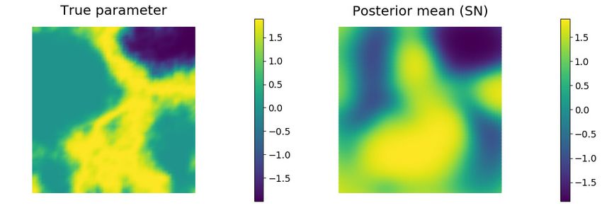
RML based posterior sampling                                                                 5

for given m̄ and do and then computes critical points of the cost functional
             1           T −1             1             T −1
 Li (m) =      (m − m0i ) CM  (m − m0i ) + (g(m) − δi0 ) CD  (g(m) − δi0 ) . (5)
             2                            2
by solving
                                      ∇m Li (m) = 0,                                       (6)
for m. Dropping the subscript i, this leads to a map from (m, δ) to (m0 , δ 0 )
defined by          (
                                          −1
                      m0 = m + CM GT CD      (g(m) − δ)
                       0
                                                                         (7)
                      δ =δ
which we denote compactly as

                                         z 0 = Ψ (z),                                      (8)

where z = (m, δ), z 0 = (m0 , δ 0 ) and the differential of g is denoted G = Dg(m).
The mapping (8) is, in general, not invertible and, hence, a single draw (m0i , δi0 )
from (4) can lead to multiple critical points (mj , δj ).1 We therefore introduce
the set-valued
                                    Mz0 = Ψ −1 (z 0 )
and denote its elements by zj (z 0 ) ∈ Mz0 , j = 1, . . . , n(z 0 ), where n(z 0 ) denotes
the cardinality of Mz0 . Each z leads to a unique z 0 , hence the sets Mz0 are
disjoint. Let us denote the set of all z 0 for which n(z 0 ) > 0 by U and let us
assume for now that U agrees with the support of the distribution qM 0 ∆0 .2
    A distribution q(z 0 ) transforms under a map (8) into a distribution p(z)
according to
                                         X p(zi )
                               q(z 0 ) =                                               (9)
                                               J(zi )
                                            zi ∈Mz0

with Jacobian J(z) = det(DΨ (z)). We will frequently use the abbreviation |A|
for the determinant det(A) of a matrix A. An explicit expression for p(z) is
obtained via
                         p(z) = n(z 0 )−1 J(z) q(z 0 )
for all z ∈ Mz0 , which satisfies (9). In the original notation and employing
(7), the transformed distribution pM ∆ is given by

   pM ∆ (m, δ) := n(m0 )−1 qM 0 ∆0 (m0 , δ 0 ) J(m, δ)
                                            −1
                 = n(m0 )−1 qM 0 m + CM GT CD

                                               (g(m) − δ) q∆0 (δ) J(m, δ) .

Here n(m0 ) is the total number of critical points of (5) for each (m0 , δ 0 ) and
J(m, δ) denotes the Jacobian determinant associated with the map (m, δ) →
  1 See Sec. 3.1 for a sampling problem with a quadratic observation operator, g, resulting

in a non-invertible mapping. In that example, (7) is cubic in the variable m. Non-invertible
mappings appear to be common for Darcy flow problems (e.g., Sec. 3.3.3).
  2 If there are points z 0 for which M 0 is the empty set, that is, n(z 0 ) = 0, we adjust the
                                          z
PDF qM 0 ∆0 such that qM 0 ∆0 (z 0 ) = 0 for Mz0 = ∅.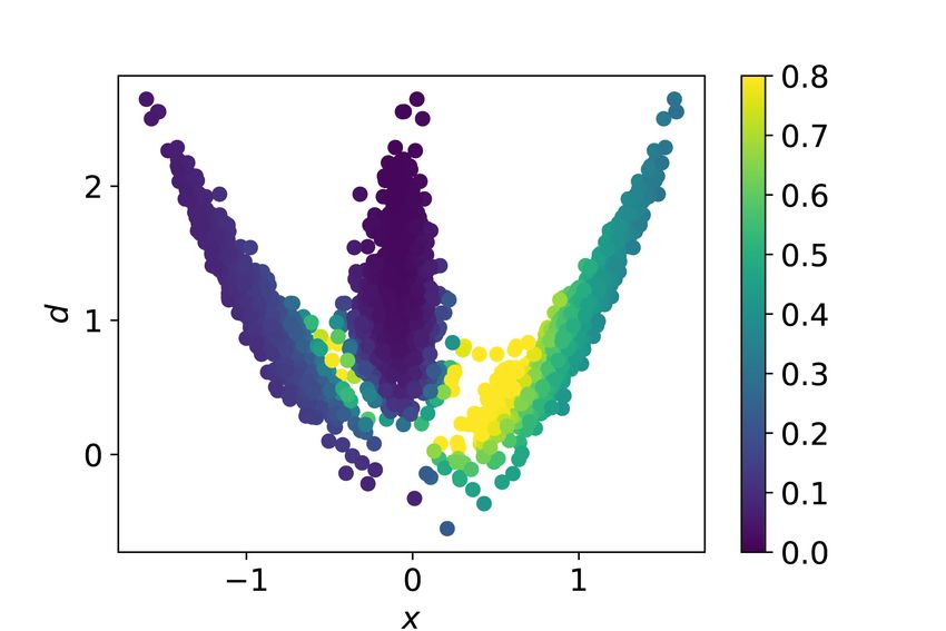
6                                        Y. Ba, J. de Wiljes, D. S. Oliver and S. Reich

(m0 , δ 0 ). In the following, we assume that J 6= 0 everywhere, i.e., the map is
locally invertible. The Jacobian matrix is provided by
                                                     −1

                              I + Db(m, δ) −CM GT CD
                                                                             (10)
                                    0           I
                          −1
with b(m, δ) = CM GT CD      (g(m) − δ).
    Hence, given samples, (m0i , δi0 ), from (4) we can easily produce samples,
(mk , δk ), from the distribution pM ∆ (m, δ) and would like to use them as im-
portance samples from the target distribution πM (m) := πM (m|do ) as defined
by (2). Note that the target density πM (m) does not specify a distribution in
δ and we will explore this freedom in the subsequent discussion in order to
define an efficient importance sampling procedure.
    Indeed, we may introduce an extended target distribution by
                         πM ∆ (m, δ) := πM (m) π∆ (δ|m)
without changing the marginal distribution in m. The conditional distribution
π∆ (δ|m) will be chosen to make the proposal density similar to the target
density, i.e.,
                             πM ∆ (m, δ) ≈ pM ∆ (m, δ).
We will find that equality can be achieved for linear forward maps, g(m) = Gm.
In all other cases, samples, (mk , δk ) from pM ∆ (m, δ) will receive an importance
weight
                                        πM ∆ (mk , δk )
                                wk ∝                                           (11)
                                        pM ∆ (mk , δk )
                             PNe
subject to the constraint k=1       wk = 1. Note that all involved distributions
need only to be available up to normalisation constants which do not depend
on m or δ.
    The subsequent discussion will reveal a natural choice for π∆ (δ|m) and will
lead to an explicit expression for (11). Let us therefore go through the analysis
to factor
                    pM ∆ (m, δ) = n(m0 )−1 qM 0 ∆0 (m0 , δ 0 ) J(m, δ)
to determine a candidate π∆ (δ|m). First, we expand the negative log density
− log qM 0 ∆0 , ignoring the normalization constant:
    1                  −1
                                    T −1                       −1
      m − m̄ + CM GT CD                        m − m̄ + CM GT CD

                          (g(m) − δ) CM                             (g(m) − δ)
    2
                            1         T −1
                         + (δ − do ) CD       (δ − do )
                            2
      1        T −1              1
    = (m − m̄) CM    (m − m̄) + (g(m) − δ)T Cd−1 GCM GT CD     −1
                                                                  (g(m) − δ)
      2                          2
           1                              1          T
        + (g(m) − δ)T Cd−1 G (m − m̄) + (m − m̄) GT CD    −1
                                                             (g(m) − δ)
           2                              2
         1          T −1                    1           T −1
      + (g(m) − do ) CD     (g(m) − do ) + (g(m) − δ) CD      (g(m) − δ)
         2                                  2
           1         T −1                   1            T −1
        − (g(m) − δ) CD      (g(m) − do ) − (g(m) − do ) CD     (g(m) − δ) .
           2                                2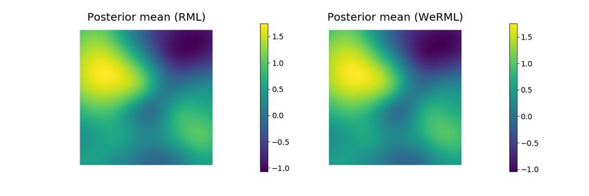
RML based posterior sampling                                                 7

To simplify the notation we will use

                               V := CD + GCM GT                          (12)

and
                      η(m) := G(m − m̄) − (g(m) − do ).                  (13)
Then, using the new definitions to simplify notation, we obtain
 pM ∆ (m, δ) =
                                    πM (m)
 z                          }|                             {
         1        T −1          1         o T −1         o
 A0 exp − (m − m̄) CM (m − m̄) − (g(m) − d ) CD (g(m) − d )
         2                      2
                                        π∆ (δ|m)
        z                                  }|                         {
               1/2       1                 −1
                                               T                −1

      × A1 |V | exp − δ − g(m) − V η(m) V δ − g(m) − V η(m)
                         2

                                         1
             × n(m0 )−1 A2 |V |−1/2 exp η(m)T V −1 η(m) J(m, δ),
                                         2
                                                                    (14)
where A0 , A1 , and A2 are all normalisation constants,
                                                  R      independent of m and
δ. A0 is determined from the requirement that R     π M (m) dm = 1. Similarly,
A1 is determined from the requirement Rthat π∆ (δ|m) dδ = 1. Finally, A2 is
determined from the requirement that pM ∆ (m, δ) dm dδ = 1. The last line
of (14) is exactly the difference between the proposal density and the target
density, which determines the importance weights (11).
    Note that if the observation operator is linear, then n(m0 ) = 1 and all
terms on the last line of (14) are independent of m so the target and proposal
densities are equal: pM ∆ = qM ∆ .

2.2 Weighting of RML samples

To weight the RML samples, we compute the weights by
                                  πM (mk ) π∆ (δi |mk )
                           wk ∝
                                    pM ∆ (mk , δk )
with π∆ (δ|m) as defined in (14). So the weight on a sample is

                                     1
           w ∝ n(m0 ) |V |1/2 exp − η(m)T V −1 η(m) J −1 (m, δ).         (15)
                                     2
The Jacobian determinant and the gradient of the misfit term with respect
to the parameter are necessary for the computation of weights. For the low-
dimensional space, it is easy to calculate them. However, the computation of
the Jacobian determinant and the gradient is difficult when the problems are
strongly nonlinear.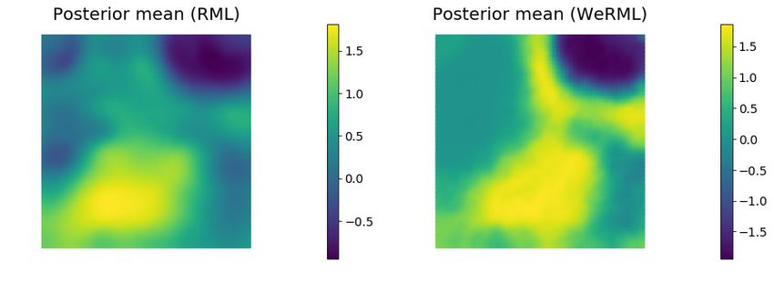
8                                        Y. Ba, J. de Wiljes, D. S. Oliver and S. Reich

   In this section, we use the low-rank approximation to get the Jacobian de-
terminant and det V . Using the Gauss-Newton approximation for the Jacobian
matrix given by (10), we have
                                              −1
                        J(m, δ) ≈ |I + CM GT CD  G|

and J becomes independent of δ. Let mMAP and Hmisfit denote the minimizer
point of (6) and the Hessian matrix of Li (m) with respect to the misfit term
at mMAP , respectively. Thus the Hessian matrix of Li (m) at mMAP is given
by
                                     −1
                           Hmap = CM    + Hmisfit .
To compute its determinant, we would like to approximate Hmap with a rel-
atively small number of terms. Thus we solve the following generalized eigen-
value problem (GEP): find U ∈ RNm ×Nm and Λ = diag(λi ) ∈ RNm ×Nm , which
are the generalized eigenvectors and eigenvalues of the matrix pair Hmisfit and
  −1
CM   , respectively:
                                           −1
                             Hmisfit U = CM   U Λ,
such that
                   −1                                −1         −1
              U T CM  U =I     and        Hmisfit = CM  U ΛU T CM  .

   For the large-scale flow problem, we consider the Whittle-Matérn prior
covariance operator based on the inverse of an elliptic differential operator,

                   Cprior = (−γ∆ + αI)−2 ,
                                         !                    !
                              1      r                   r                        (16)
                          =       p        K1         p
                            4πγα    γ/α                γ/α

where K1 denotes the modified Bessel function of the second kind of order
1. Eq. (16) provides a sparse representation of the inverse covariance and a
square root factorization that is useful for computing a low-rank approximation
                                                                         −1
of the Hessian matrix [8]. From (16) the variance is pseen to be (4παγ) and
the range of the covariance to be proportional to γ/α. CM is given by the
discretization of Cprior and the inverse of CM can be easily factored
                                 −1
                                CM  = QQT .

So we have

             Hmap = QQT U ΛU T QQT + QQT = QÛ (Λ + I)Û T QT ,

where Û = QT U is the matrix of orthonormal eigenvectors for Q−1 Hmisfit Q−T .
We actually want the determinant
                                                               Nm
                                     T                         Y
        |CM Hmap | = |Q−1 Hmap Q− | = Û (Λ + I)Û T =               (1 + λi ).
                                                               i=1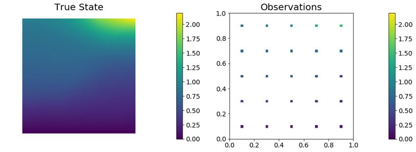
RML based posterior sampling                                                   9

When the generalized eigenvalues {λi } decay rapidly, we can use a low-rank
approximation of Hmisfit by retaining only the r largest eigenvalues and cor-
responding eigenvectors, i.e.,

                          Hmisfit ≈ QQT Ur Λr UrT QQT .

Thus we have
                                           r
                                           Y
                               J(m, δ) ≈       (1 + λi ).
                                           i=1

    We also need the determinant of V for the computation of weights in (15).
In section 3.3, we will use a diagonal matrix for CD , i.e., CD = σ 2 I. Due to
               −1
Hmisfit ≈ GT CD   G, we have

                                        −1         −1
                          GT σ −2 IG ≈ CM  U ΛU T CM  .

Then
                                                 −1
                           CM GT G ≈ σ 2 U ΛU T CM  .

The determinant of V

          |V | = |σ 2 I + GCM GT | = σ 2(Nd −Nm ) |σ 2 I + CM GT G|
                                                                        −1
                                    ≈ σ 2(Nd −Nm ) |σ 2 I + σ 2 U ΛU T CM  |
                                    = σ 2Nd |I + QT U ΛU T Q|
                                    = σ 2Nd |I + Û ΛÛ T |
                                             Yr
                                    ≈ σ 2Nd     (1 + λi ).
                                             i=1

Thus the determinant of V can be also replaced by a low-rank approximation.
σ 2Nd is not necessary in |V | because it appears in all weights and can be
factored out. Then (15) can be approximated by
                                      Yr
                      0    1    T −1
            w ∝ n(m ) exp − η(m) V η(m)    (1 + λi )−1/2 .
                           2            i=1

    In the approach described above, the computation of G for the weights is
necessary. To obtain G for the flow problem in section 3.3, we solve an adjoint
system [42]. In section 3.1, we investigate the effect of a Gauss-Newton ap-
proximation for the weights for cases in which all the critical points and only
minimizers of (6) are obtained, respectively. As the Gauss-Newton approxima-
tion of the weights is shown to be poor for maximizers of the objective function,
we only consider the minimizers in the Darcy flow example (Sec. 3.3).
10                                        Y. Ba, J. de Wiljes, D. S. Oliver and S. Reich

2.3 Weighted RML sampling algorithm

In this section, we consider two possible situations when seeking independent
samples from (2) for a log-posterior of the form (3). In both cases, we allow for
the possibility that the stochastic cost function (5) is nonconvex. Note that
in this case the number of critical points may be greater than 1. In the first
algorithm, we assume that all critical points can be identified, while in the
second case, we suppose that it is only possible to identify a single critical
point, but that the total number of critical points is unknown.

2.3.1 All critical points found

For problems in low dimensions, with polynomial observation operators g, or
convex cost functions, it may be feasible to find all critical points for each pair
(m0 , δ 0 ). If the ith sample of (m0 , δ 0 ), generates a cost function Li (m) with
nci critical points, it is possible to sample correctly by weighting each critical
point using (15).

 Algorithm 1: Weighted RML – computing all the critical points
     i = 1, k = 1
     while k ≤ Ne
         generate samples m0i and δi0 from qM 0 ∆0 (m0 , δ 0 )
         for j = 1 to nci
              solve (6) for m(j) and set δ (j) = δi0
              compute w(j) using (15)
              assign mk = m(j) and wk0 = w(j)
              k =k+1
         i=i+1
     assign wk = wk0 / k wk0
                        P

    Note that when the forward operator g is linear, i.e., g(m) = Gm, the
stochastic cost function is convex for each pair (m0 , δ 0 ). The log-posterior has a
single critical point, which is the minimizer. Thus, for linear forward operators,
we just need to compute the minimizers and the weights are all equal by using
(15).

2.3.2 One critical point found

Finding all the critical points is not feasible when the problem dimension and
the complexity increases. In these cases, it is unlikely that even the number
of critical points will be known. Instead of seeking to compute all critical
points, we compute a single critical point using a random starting point for the
optimization. We assume, without evidence, that the optimization performed
this way uniformly samples the critical points, in which case the resulting
RML based posterior sampling 11
Pnc
j=1 m(j) w(j) provides an unbiased estimator in the same manner as it is
obtained from computing all critical points.
Algorithm 2: Weighted RML – sample one critical point
for i = 1 to Ne
generate samples m0i and δi0 from qM 0 ∆0 (m0 , δ 0 )
randomly generate minit (initial guess)
solve (6) for mi and set δi = δi0
compute wi0 using 0
P 0(15) with n(m ) = 1
0
assign wi = wi / i wi
2.3.3 Local minimizers only
Due to the high dimension of most realistic applications, solutions of (6) are
much more difficult to obtain than local minimizers of L, although local max-
imizers can clearly be easily found as minimizers of −Li . In general, however,
it appears that in high dimensions, minimizers of Li are far more important
than maximizers. When that is the case, a Gauss-Newton approximation of
the Jacobian determinant can be made with little loss of accuracy
−1
J = |I + D(CM GT CD (g(m) − δ))|
−1
≈ |I + CM GT CD G| .
Thus, in the Darcy flow problem, we will solve for random minimizers
instead of solving for random critical points and we will compute a Gauss-
Newton approximation of the Jacobian determinant. The consequence of this
approximation is that the distribution of samples will not be exact. In section
3.1, we investigate numerically the consequence of sampling only the minimiz-
ers.
To obtain the weights, the computation of the Jacobian determinant and
the gradient of the misfits with respect to the parameter are necessary. For
the first two examples, it is easy to compute the weights. For the large-scale
flow problem, we use the Gaussian-Newton method in the hIPPYlib [42] to
get a low-rank approximation of the Jacobian determinant. This can reduce
the cost.
3 Numerical examples
In this section, we present sampling results using test cases of increasing size
and complexity. We first demonstrate the methodology using a toy problem
that has been previously used by [44]. It is small enough that the true poste-
rior distribution is easily derived. We focus on the parameter values that are12 Y. Ba, J. de Wiljes, D. S. Oliver and S. Reich
difficult to sample correctly. This example shows the difficulty with using only
the minimizers and not accounting for the limited range in the solutions.
A second simple example is the “banana-shaped” distribution from [18]. It
has been used fairly often to test adaptive forms of MCMC [19, 43, 37, 30, 12]. It
is simple enough that computing the Jacobian determinant is not a challenge
so the focus again is on showing that if we find the roots and compute the
weights, the sampling is correct.
3.1 Bimodal posterior pdf
The first example has been previously discussed in [44] where it was used
to demonstrate properties of the randomized maximum a posteriori sampling
algorithm. One of their test problems required sampling from the distribution
1 2 1 2 2
πM (m) ∝ exp − (m − 0.8) − 2 (m − 1) .
2 2σd
Although [44] used three different values of σd , we only show results for the
most difficult value, σd = 0.5. For larger and smaller values, the posteriori
distribution is more easily modeled as a mixture of Gaussians and is therefore
easier to sample.
In our approach, approximate samples from the posteriori distribution are
obtained by solving for the critical points of
1 1
Li (m) = (m − m0i )2 + 2 (m2 − δi0 )2 (17)
2 2σd
m0i ∼ N (0.8, 1) δi0 ∼ N (1, 0.25).
Because the objective function in this case is a polynomial, it is straightforward
to obtain all real roots of (6). For most choices of (m0 , δ 0 ) there are three real
roots – Ns = 10, 000 samples of (m0 , δ 0 ) from the prior generated Ne = 25, 046
pairs of (m, δ). The locations of the roots are shown in Figure 1a. The set
of points in the center of the plot correspond to maximizers of (17). The
points on the right side correspond to the global minimum, and the points
on the left correspond to the local minimum. The colors show unnormalized
importance weights for each sample. The maximizers are generally given small
weights (Fig. 1b), although a small number of maximizers have weights that
are similar to the weights of points near the local minimum.
Because the samples are generated independently (or in groups of three),
the quality of the weighted sampling approximation to the target distribution
is limited only by sampling error – larger samples provide better approxima-
tions. Figure 2 shows results for three different sample sizes Ns (200, 1000,
5000). The number of weighted samples is larger than the ensemble size be-
cause a single sample from the prior usually results in three critical points.
For this problem, computing all real roots of (6) and computing importance
weights for each root is trivial. For large high-dimensional problems, findingRML based posterior sampling 13
minimizer
12.5 maximizer
10.0
7.5
5.0
2.5
0.0
0.0 0.2 0.4 0.6 0.8 1.0
Weight
(a) Solutions of ∇Li (m) = 0. Color indi- (b) Distribution of weights from critical
cates importance weight. points.
Fig. 1 Critical points and importance weights for the quadratic observation operator.
1.2 1.2
1.0 1.0
1.0
0.8 0.8 0.8
0.6 0.6 0.6
0.4 0.4 0.4
0.2 0.2 0.2
0.0 0.0 0.0
−1.5 −1.0 −0.5 0.0 0.5 1.0 1.5 −1.5 −1.0 −0.5 0.0 0.5 1.0 1.5 −1.5 −1.0 −0.5 0.0 0.5 1.0 1.5
(a) Ns = 200. (b) Ns = 1000. (c) Ns = 5000.
Fig. 2 Weighted sampling approximations to the true posterior distribution.
multiple roots and computing the weights will be challenging. Here we ex-
amine the consequence of three realistic approximations to correct sampling:
(1) identifying only the minimizers of the cost function, (2) using a Gauss-
Newton (GN) approximation of the Jacobian of the transformation and (3)
neglecting importance weights altogether. Fig. 3c shows that correct sampling
of the target distribution is obtained when all critical points are included and
the weights are computed accurately. If the importance samples are neglected
(Fig. 3a) or if the GN approximation of the Jacobian is used (Fig. 3b), the
distribution of samples is badly distorted. When it is not possible to compute
the Jacobian accurately in high dimensions, it appears to be advisable to only
compute the minimizers. The distribution of samples obtained using the GN
approximation applied to minimizers (Fig. 3e) is nearly as good as the results
with correct weights, and far better than results with no importance weighting.14 Y. Ba, J. de Wiljes, D. S. Oliver and S. Reich
no importance weights GN approx weighted
1.2
(a) (b) (c)
all critical pts
1.0 1.0
1.0
0.8 0.8 0.8
0.6 0.6 0.6
0.4 0.4 0.4
0.2 0.2 0.2
0.0 0.0 0.0
−1.5 −1.0 −0.5 0.0 0.5 1.0 1.5 −1.5 −1.0 −0.5 0.0 0.5 1.0 1.5 −1.5 −1.0 −0.5 0.0 0.5 1.0 1.5
1.0 (d) 1.2 (e) 1.2
(f)
1.0
1.0
minimizers
0.8
0.8
0.8
0.6
0.6 0.6
0.4
0.4 0.4
0.2 0.2
0.2
0.0 0.0 0.0
−1.5 −1.0 −0.5 0.0 0.5 1.0 1.5 −1.5 −1.0 −0.5 0.0 0.5 1.0 1.5 −1.5 −1.0 −0.5 0.0 0.5 1.0 1.5
Fig. 3 Compare distributions from approximations to sampling based on computation of
critical points of cost function.
3.2 Banana-shaped posterior pdf
The second numerical example is the widely used “banana-shaped” target
density initially presented in [18], but extended to higher dimensions by [37],
1 1
πM (m) ∝ exp − 2 m21 + m22 + · · · + m2Nm exp − 2 (4 − 10m1 − m22 )2
2σm 2σd
(18)
with σd = 4 and σm = 5. In our numerical experiment, we use parameters
values from [30], but increased the dimension of m to 4. The first term of (18)
is identified as the Gaussian prior with model covariance CM = I and the
second term as the log-likelihood, with
g(m) = 10m1 + m22 .
Because of the curved shape of the objective function (Fig. 5b), accurate
computation of minimizers of Li was relatively difficult. Three projections
of the first 3000 approximate samples obtained using the Broyden-Fletcher-
Goldfarb-Shanno algorithm for minimization are shown in Fig. 4. Each mini-
mization was initiated at the point m0i .
For this problem, which has a single critical point, the empirical distri-
bution obtained from minimization appears to be relatively good. The true
conditional distribution distribution π(m1 , m2 |m3 = 0, m4 = 0) is compared
in Fig. 5b, with a kernel estimate of the empirical marginal distribution for
m1 , m2 (dashed contours) obtained using 50,000 minimizations. Also, based
on the distribution of unnormalized importance weights (Fig. 5a), it appears
that the weights are not dominated by a few large values, which is confirmed
by a high effective sampling efficiency, Neff /Ne = 44796/50000 ≈ 0.9, based
on Kong’s estimator (19),
1
NEff = PNe , (19)
k=1 wk2RML based posterior sampling 15
(a) m1 -m2 plane. (b) m1 -m3 plane. (c) m1 -δ plane.
Fig. 4 Critical points of the banana-shaped objective function. Color indicates importance
weight on the samples. The same color scale is applied to all subplots.
PNe
where k=1 wk = 1
300
200
100
0
0.000 0.002 0.004 0.006 0.008 0.010 0.012
Weight
(a) Distribution of importance weights for the min- (b) Compare true distribution
imizers of the log posterior. with estimation from weighted
minimizers (m1 -m2 plane).
Fig. 5 Minimizers of the banana-shaped objective function.
3.3 Darcy flow example
For the first two examples, there would be no advantage in using RML for
sampling – MCMC with a carefully chosen transition kernel would probably be
a better alternative in either case. The advantage for RML occurs in large high-
dimensional problems for which traditional methods are impractical. In this
section, we investigate the ability to quantify uncertainty in the permeability
field κ(x) from spatially distributed observation of steady-state pressure. The16 Y. Ba, J. de Wiljes, D. S. Oliver and S. Reich
pressure u(x) in this example is governed by the equation
−∇ · (κ(x)∇u(x)) = 0 in Ω = [0, 1] × [0, 1]
with the mixed boundary conditions
∇u · n = 0 on ΓN1 = 0 × [0, 1] ∪ 1 × [0, 1]
∇u · n = v(x) on ΓN2 = [0, 1] × 1
u(x) = 0 on ΓD = [0, 1] × 0.
As permeability is a positive quantity, it cannot be modelled as a Gaussian
random variable. Here, we evaluate sampling with three possible prior distri-
butions for permeability. In all cases, we define a latent variable m(x) that
is multivariate Gaussian, with a prior given by (16). We take α = 0.12 and
γ = 1.12 which results in a correlation length of approximately 2 and a variance
of 1. In the first case (Case 1), permeability
is modeled as being log-normally
distributed, i.e., κ(x) = exp m(x) , which is a typical assumption for the
distribution of permeability within a single rock type [15]. In more complex
formations, it is often useful to model permeability as being largely determined
by rock type. In that case, permeability might be largely uniform within a rock
type, but variable between rock types. We created two soft thresholding trans-
formations to model the distribution of permeability in a formation with three
rock types. In the the first of the distributions (Case 2), the permeability
is related to the latent variable through a highly nonlinear, but monotonic
transformation
κ(x) = exp tanh 4m(x) + 2 + tanh 4m(x) − 2 . (20)
In the second distribution (Case 2), the permeability is related to the latent
variable through a non-monotonic transformation
κ(x) = exp 2 tanh 4m(x) + 2 + tanh 2 − 4m(x) − 1 , (21)
which gives a permeability field with a low permeability ‘background’ and
connected high perm ’channels’ as might occur in subsurface rock forma-
tions [2]. Figure 6 shows the transformations and the three synthetic true
log-permeability fields that are used to generate observations for Case 1 (top
right), Case 2 (lower left) and Case 3 (lower right).
Figure 7 (left) shows the true pressure field for Case 1. The pressure distri-
butions for Cases 2 and 3 look similar. For each case, we take 25 pressures as
observations. The observation locations are distributed on the uniform 5 × 5
grid of the domain [0.1, 0.9] × [0.1, 0.9] as shown in Figure 7 (right). The noise
in the observations is assumed to be Gaussian and independent with standard
deviation 0.01. For the mixed boundary condition, we take v(x) = 2 for Case 1
and 0.7 for Case 2. Here the piecewise quadratic finite element is used for the
state and adjoint spaces, while piecewise linear finite element is used for the
parameter space. The forward model is solved by the finite element methodRML based posterior sampling 17
(a) Three transformations (b) Case 1
(c) Case 2 (d) Case 3
Fig. 6 The true log-permeability fields for Cases 1, 2 and 3. All cases use the same true
latent variable field.
Fig. 7 The true state (left) and observation locations (right).
with a uniform 50 × 50 grid for the three cases. Thus the dimension of the
discrete state and adjoint space is 10201 and the dimension of the parameter
space is 2601.
We used the hIPPYlib environment [41, 42] for computation of low-rank
approximations of eigenvalues of the Hessian. hIPPYlib builds on FEniCS
[27, 22] for the discretization of the PDE and uses PETSc [1, 47] for scalable
and efficient linear algebra operations and solvers. Minimizers of the objective
functions are computed using an inexact Newton-CG solver. We used default
parameters for minimization, except that we increased the maximum number18 Y. Ba, J. de Wiljes, D. S. Oliver and S. Reich
of iterations to 300. The actual average number of iterations required for con-
vergence varied considerably for the three cases. In Case 1, an average of 24
iterations were required, Case 2 required 34 iterations and Case 3 required an
average of 73 iterations.
For the Darcy flow examples, the low-rank approximation of the Jacobian
determinant J was used to reduce the cost of computation of weights. The low-
rank approximation adopts the Gauss-Newton method in the hIPPYlib [42].
To illustrate the performance of the proposed method, we compare the results
obtained by using the stochastic Newton method [29] implemented in hIPPYlib
with that of unweighted RML and weighted RML. Here the stochastic Newton
samples are generated from the Gaussian approximation of the posterior. The
observation data, prior covariance operator and sample size Ne are the same
for the RML and stochastic Newton methods. For convenience, we write the
stochastic Newton as SN, unweighted RML as RML and weighted RML as
WeRML in the figures of the three cases.
3.3.1 Case 1: permeability field is log-normal
As the permeability transformation, κ = exp m, is monotonic in this example,
we might expect the stochastic cost function Li to have a single critical point
for each sample from the prior. We confirmed this empirically through an
investigation in which we generated a single sample from the prior, but 50
randomly sampled starting points for the minimization. In the experiments,
all 50 initial starting models converged to the same model parameters. In
the results that we present, RML sampling was performed with 1000 samples
from the prior and a single random starting point for each minimization. We
dropped 15 out of 1000 samples for which the minimization routine failed to
converge to a sufficiently small value of the gradient norm in 300 iterations.
The effective sample size computed from (19), was relatively high for this
case: Neff ≈ 823 effective samples. The effective sample efficiency, Neff /Ne =
823/985 = 0.836. Unlike the toy examples, computing the minimizers and the
Jacobian determinant is necessarily approximate in the Darcy flow problem.
The expected value for the squared data misfit (with respect to the actual
observed values of pressure) is nd σd2 = 0.0025, which is somewhat smaller
than the mean of the actual squared misfits, 0.0032.
Figure 8a shows crossplots of the weights vs squared data misfit computed
using V as in (12). The approximation of log-weights is only slightly correlated
with the squared data misfit (r = −0.09) so it appears that in this case, as
in the quadratic example, the data mismatch would not serve as a viable
surrogate for weighting of samples. In addition to data mismatch, the weights
are affected by the nonlinearity of the problem – either through |V | or through
the term (g(m) − Gm), which occurs in η.
In Fig. 9, we plot the distribution of sample values of the latent variable at
three locations for which the true field has values m = 1.7, 0.04 and −1.17. For
this example, the marginal distributions of samples at observation locationsRML based posterior sampling 19
(a) Case 1 (lognormal permeability) (b) Case 2 (monotonic log-permeability)
Fig. 8 The weights vs misfits for the minimizers. Blue points show computed weights.
from unweighted RML, SN and weighted RML are all similar and approxi-
mately Gaussian.
Estimates of the posterior mean of the log-perm field from three different
sampling approaches are shown in Fig. 10. As the permeability field is a mono-
tonic function of the latent variable for this case, the estimated conditional
means of the log-perm fields are similar for the three methods.
Despite the similarity of the mean fields and the similarity of the estimates
of the posteriori standard deviation from the three methods, the realizations
from the three methods are not as similar in their ability to reproduce data
(Fig. 11). The mean squared data misfit for weighted RML is 0.0032, while
the mean squared data misfit for stochastic Newton is 0.0048. This is similar
to the observation of Liu and Oliver [25] who showed that the data mismatch
of realizations generated from the posteriori mean and covariance in a 1D
Darcy flow problem were much larger than data mismatch from MCMC or
from RML.
3.3.2 Case 2: log-permeability is monotonic function of latent variable
Although it is common to assume that permeability is log-normally distributed
within a single rock type, in many subsurface formations the distribution of
permeability is largely controlled by ‘rock type’. In Case 2 we model the spatial
distribution of rock types by applying a soft threshold to a latent Gaussian ran-
dom field. With this transformation, values of m < 1 are assigned log κ ≈ −2
and values values of m > 1 are assigned log κ ≈ 2. One practical consequence
of this transformation is that minimization of the objective function is more
difficult. The second, more important consequence is that the nonlinearity in
the neighborhood of the minimizers increases the variability in weights. So
while in Case 1, approximately 90% of the weights were between 0.0006 and
0.0015, in Case 2 approximately 90% of the weights fell between 10−4 and
9 × 10⁻³ (Fig. 8b). The effective sample size for the 930 samples that con-
verged successfully is also smaller in this case; Neff = 179 for an efficiency of
about 19.2%.20 Y. Ba, J. de Wiljes, D. S. Oliver and S. Reich Fig. 9 Density histograms of samples of the latent variable at locations (0.1,0.5), (0.5,0.1) and (0.9,0.9) using SN (upper row), unweighted RML (middle row) and weighted RML (lower row). As the posterior distribution is not even approximately Gaussian, the mean and variance may not be the best attributes for judging the quality of the data assimilation. It is common in inverse problems to judge the quality of the realizations by the data misfit after calibration. The expected value of the mean squared data mismatch with observations is 0.0025. The value computed from weighted RML (0.0029) is quite close to that value. In contrast, the value from SN realizations (0.0087) is about 3.5 times larger than expected and the value from unweighted RML (0.0033) is slightly larger than weighted RML. The distributions of squared data misfits for the three methods are shown in Fig. 12a.
RML based posterior sampling                                                            21

Fig. 10 The true log-permeability field for Case 1 (upper left) and the posterior mean log-
permeability fields from three approximate sampling methods: stochastic Newton (upper
right), RML without weighting (lower left) and RML with GN approximate weighting (lower
right).

Fig. 11 Distributions of squared data misfit from samples generated using SN and using
weighted RML.

3.3.3 Case 3: log-permeability is non-monotonic function of latent variable

Applying the transformation (21), we obtain a permeability field with a low
permeability ‘background’ and connected high perm ‘channels’. The ‘true’ la-
tent variable field and the corresponding true log-permeability field are shown
in Fig. 6. The true pressure field, from which data are generated, and obser-
vation locations are plotted in Fig. 13.
    In this example, the transformation from the Gaussian latent variable to
the permeability variable is highly nonlinear and non-monotonic, so we should
22 Y. Ba, J. de Wiljes, D. S. Oliver and S. Reich
(a) Case 2 (monotonic log-permeability) (b) Case 3 (non-monotonic log-
permeability)
Fig. 12 Compare distributions of squared data misfit for three sampling methods: RML,
weighted RML (WeRML), and stochastic Newton (SN).
Fig. 13 The true state (left) and observation locations (right)
expect to encounter two problems: convergence to the minimizer will be slow
[26] and the algorithm is likely to converge to a local minimum that does not
have large probability mass associated with it.
We focus on the distribution of samples that are obtained using a practice
that could feasibly be applied to large-scale subsurface data assimilation prob-
lems if a gradient is available – search for a single minimizer for each sample
from the prior and use the Gauss-Newton approximation of the Jacobian to
compute the weights. Here we have taken 1000 samples from the prior and per-
formed 1000 corresponding minimizations, from which we obtained Ne = 885
samples with successful termination and weights. Using (19), we compute the
effective sample size NEff ≈ 14. Because of the dimensionality of the problem,
it is not possible to completely characterize the posterior distribution for either
the latent variables, or for the log-permeability. In order to gain some under-
standing, we examine the marginal distribution of the minimizers at three
observation locations for which the true log-permeability values are approxi-
mately, -2, 0 and 2. The marginal distribution of unweighted minimizers (upper
row Fig. 14) is bimodal at two of the observation locations. The lower row ofRML based posterior sampling 23
Fig. 14 (lower row) shows the corresponding distribution of unweighted log-
permeability values at the same locations. Although the spread of m is fairly
large at each of the observation locations, the spread of the log-permeability
values are tightly centered on −2, 0 and 2 in Fig. 14 (lower row). This is a
consequence of the thresholding property of the log-permeability transform.
Fig. 14 Density histograms of values of the minimizers of the objective functions at three
observation locations (upper row) and corresponding values of the log-perm field (lower
row). Colors separate minimizers into two groups by weight.
The colors used for the density histograms in Fig. 14 separate the samples
into two groups: one in which w > 10−9 and the second for which w < 10−9 .
Note that in Fig. 14 (lower right), a substantial fraction of samples converged
to a local minimizer with log κ ≈ 0 at x, y = (0.9, 0.9), which is far from the
true value, log κtrue ≈ −2. Many of the clearly erroneous minimizers are easily
eliminated, however, by the low weights. Note that the inefficiency of the sam-
pling in this case is a result of the non-monotonic nature of the permeability
transform – to get from log κ = 0, which is a local minimizer, to the correct
root log κ = −2 it is necessary to pass through the point log κ = 2. In the
histograms, the samples with high weights (blue bars) are generally close to
the true values (red dashed line), which is as we expected.
As in the previous case, the expected value of the squared data misfit with
the actual observation is approximately 0.0025 at the global minimizer of the
stochastic cost function. This is close to the values that are obtained in the
best minimizations (Fig. 15 (right)). In this example, however, many of the24 Y. Ba, J. de Wiljes, D. S. Oliver and S. Reich
Fig. 15 The weights vs misfits for the minimizers of the stochastic cost function.
minimizations converged to minimizers with much larger misfit values (Fig. 15
(left)). The minimizations with large misfit values result from convergence to
local minima in the cost function. The number of local minima with large
numbers of samples appears to be relatively small as a result of the large
correlation range for the latent permeability variable. For this example, it
appears that many of the unwanted local minimizers could be eliminated either
through the weighting, or through the magnitude of the squared data misfit.
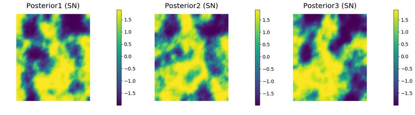
Figure 16 compares distributions of the values of the log-permeability field
obtained by the SN and the weighted RML methods at three pressure ob-
servation locations. For consistency, the same sample size was used for both
methods. The true values of the log-permeability field at the observation lo-
cations are close to −2, 0 and 2 (shown as small red dots). When using the
weighted RML samples to approximate the distribution, the samples are seen
to be concentrated close to the true values at the three observation locations
(Fig. 16 (lower)). Because of the highly nonlinear transformation of the per-
meability field, the SN method was unable to provide a good approximation
to the true posterior distribution, although it did provide plausible estimates
of uncertainty in log κ at two of the locations. At the third location (upper left
in Fig. 16) the uncertainty in log-permeability was completely misrepresented.
Although the marginal distribution of the log-permeability field is mul-
timodal at some locations before and after data assimilation, the mean of
log-permeability is useful for qualitatively gauging the quality of the data
assimilation. In Fig. 17, we compare the MAP point of SN, and the un-
weighted and weighted posterior means of RML with the true log-permeability
field. All three methods provide reasonable characterization of the mean log-
permeability in the upper right area of the grid, but only the weighted RML
method adequately characterizes log-permeability on the left side. It appears
that it would be risky to use results from RML without weighting in this case.
As the posterior distribution is multi-modal, the mean and variance may
not be the best attributes for judging the quality of the data assimilation. Two
qualitative criteria are often used in practice. First, it is common to judge the
quality of the realizations by the data misfit after calibration. The expected
value of the mean squared data mismatch with observations is 0.0025. TheRML based posterior sampling 25
Fig. 16 The histograms of values of the log-perm field at three observation locations by
using the SN (upper row) and weighted RML (lower row) methods.
value computed from weighted RML is quite close to that value, 0.0029. In
contrast, the value from SN realizations is about 10 times larger than expected
(0.0264) and the value from unweighted RML is larger still (0.0486). The dis-
tributions of squared data misfits for the three methods are shown in Fig. 12b.
Second, the samples themselves can be examined qualitatively for ‘plausibil-
ity’ – do they look like samples from the prior? Fig. 18 shows RML samples
with largest weights (bottom row) and the corresponding posterior samples for
SN (top row). In this case, the weighted and unweighted RML samples look
plausible, but the samples from SN do not.
3.4 Discussion of porous flow results
The porous flow examples were chosen to be large enough that a naı̈ve ap-
proach to particle filtering in which particles are sampled from the prior and
then weighted by the likelihood would suffer from the curse of dimensional-
ity and all the weight would fall to a single particle. The dimension of the
model space (2601 discrete parameters) was also large enough that computa-
tion of the Jacobian of the transformation from the prior distribution to the
distribution of critical points would be challenging.
Exact sampling of the posterior distribution using this methodology re-
quires either computation of all critical points of the objective function, or
random sampling of all critical points. In the porous media flow examples,26 Y. Ba, J. de Wiljes, D. S. Oliver and S. Reich Fig. 17 The true log-permeability field for Case 3 (upper left) and the posterior mean log-permeability fields from three approximate sampling methods: stochastic Newton (upper right), RML without weighting (lower left) and RML with GN approximate weighting (lower right). Fig. 18 Three posterior log-permeability samples from the stochastic Newton method (top row) and the three weighted RML samples with largest weights (bottom row). Samples can be compared with the true log-permeability distribution in Fig. 17.
RML based posterior sampling                                                   27

however, we were unable to locate any maximizers for the objective function
even for Case 3 in which the objective function had many local minima. As a
consequence, it appears that searching only for minimizers is a robust approx-
imation in high dimensions. Because we searched only for minimizers, it also
appears that the Gauss-Newton approximation of the Jacobian gave useful ap-
proximations. The terms that must be computed are then very similar to terms
that are computed in Gauss-Newton minimization of the cost function. It was
possible to compute an inexpensive estimate of the determinant of the Gauss-
Newton approximation of the Jacobian using eigenvalues of the Hessian at the
minimizers. Because the dimensions of the data space was relatively small, it
was also possible to estimate the determinant of the Jacobian using the adjoint
system. For Case 1, the estimates from the two approaches were similar, but
the differences increased as the nonlinearity increased. To evaluate the quality
of the sampling from the various methods, we used weights computed using
the adjoint system. The weights were more variable when low rank approxi-
mations were used. In that case, it was useful to account for the model error
by inflating the value of Cd used for computing weights.
    The degree of nonlinearity in the transformation from parameter to log-
permeability had a strong effect on the effective efficiency of the minimization
approach for sampling. The least nonlinear example (Case 1) had an effective
sample efficiency of 84% while the most nonlinear example (Case 3) had an
effective sample efficiency of 1.6%. It appears that the low efficiency in Case
3 was largely a result of the prevalence of many local minima in the objective
function, many of which were characterized by large data mismatch and very
small weights.
    When the posterior distribution had a single mode as in Case 1, the dis-
tribution of residual errors in the data mismatch was quite small and the
correlation between weight and data mismatch was correspondingly small
(r = −0.086). In that case, the data mismatch would not have provided a
useful proxy for weighting. In Case 2, the nonlinearity was greater but it
appears that the posterior distribution was still uni-modal. The weights did
correlate with data mismatch in that case (r = −0.485) but it appears that
the skewness of the distribution may have been the largest reason for the de-
crease in effective sample efficiency. Finally, in Case 3, the transformation from
the model parameter to log-permeability was non-monotonic and the poste-
rior distribution was characterized by a large number of local minima. Here,
the correlation between importance weight and data mismatch was almost
perfect (r = −0.999) and the data mismatch could serve as a useful tool for
eliminating samples with small weights.
    Although we did not compare the distribution of samples from weighted
RML with methods such as MCMC, we did compare with the stochastic New-
ton method because it is a practical and scalable method for approximate sam-
pling in high dimensions. For Case 1, which appears to be unimodal, the mean
log-permeability fields from SN and RML (both weighted and unweighted)
were visually similar. For Case 3, the mean permeability fields from SN and
28 Y. Ba, J. de Wiljes, D. S. Oliver and S. Reich
weighted RML are less similar, the data mismatches from SN are substantially
larger, and the samples are visually less plausible.
The documented cost of the three considered methods are substantially dif-
ferent. The computational complexity of the stochastic Newton method stems
from a single minimization to compute the MAP and the cost to generate
samples from a low-rank Gaussian approximation of the posterior. While the
sampling step contributes to the cost of the stochastic Newton, it is dominated
by minimization of the objective function. For the Darcy flow example, the
cost to generate 1000 approximate samples varied from 13 seconds for the log-
normal case to 56 seconds for the non-monotonic case.3 Note that this increase
is a result of the varying number of iterations required for the minimizer to
converge for the different settings. In case of the RML method, the cost to
generate Ne realizations is dominated by the cost to perform Ne minimiza-
tions with different cost functions. Henceforth the computational complexity
for RML can be expected to be approximately Ne times greater than the cost
for stochastic Newton method. Indeed, in our examples, the run time required
to generate 1000 samples from RML was approximately 1000 times greater,
varying from 13000 seconds for the log-normal case to 47000 seconds for the
non-monotonic case. For weighted RML, there is an additional cost incurred in
the computation of the weights. Although several of the terms in the weights
can be obtained at low cost through the same low-rank approximations that
were used for the Hessian, we chose tosolve the adjoint system Nd times to
compute the Jacobian of the data for computation of V −1 . The additional
cost for computing the weighting is thus dominated by the cost of running
the simulator an additional Nd times for each realization. Because the adjoint
system was solved to compute weights, the cost of computing weights var-
ied from 24000 seconds to 35000 seconds for 1000 samples, which was similar
to the cost of the minimization. All computational costs, including the cost
of minimization, could be reduced through careful modification of the algo-
rithms. In particular, the efficiency of the weighted RML could be improved
by tempering the objective function at early iterations to avoid convergence to
local minima with small weights. Also, the cost of computation of the weights
could be reduced by using a low-rank approximation of V as in the ensemble
Kalman filter.
4 Summary
We have presented a method for sampling from the posterior distribution
for inverse problems in which the prior distribution of model variables and
measurements errors are Gaussian. Although the method is highly efficient
when the posterior distribution is also approximately Gaussian, the target
application is to problems in which the posterior distribution is multimodal
3 Timing should be considered illustrative, but for reference all results were obtained on
a computer with a i7-5500U@2.40GHz × 4 processor with 7.5 GiB memory and a 64-bit
operating system.You can also read