Integrated multi omics analysis of ovarian cancer using variational autoencoders - Nature

Page created by Herbert Sharp
 
CONTINUE READING
Integrated multi omics analysis of ovarian cancer using variational autoencoders - Nature
www.nature.com/scientificreports

                OPEN             Integrated multi‑omics analysis
                                 of ovarian cancer using variational
                                 autoencoders
                                 Muta Tah Hira1,4, M. A. Razzaque2,4*, Claudio Angione2, James Scrivens1, Saladin Sawan3 &
                                 Mosharraf Sarkar1

                                 Cancer is a complex disease that deregulates cellular functions at various molecular levels (e.g.,
                                 DNA, RNA, and proteins). Integrated multi-omics analysis of data from these levels is necessary to
                                 understand the aberrant cellular functions accountable for cancer and its development. In recent
                                 years, Deep Learning (DL) approaches have become a useful tool in integrated multi-omics analysis
                                 of cancer data. However, high dimensional multi-omics data are generally imbalanced with too many
                                 molecular features and relatively few patient samples. This imbalance makes a DL based integrated
                                 multi-omics analysis difficult. DL-based dimensionality reduction technique, including variational
                                 autoencoder (VAE), is a potential solution to balance high dimensional multi-omics data. However,
                                 there are few VAE-based integrated multi-omics analyses, and they are limited to pancancer. In this
                                 work, we did an integrated multi-omics analysis of ovarian cancer using the compressed features
                                 learned through VAE and an improved version of VAE, namely Maximum Mean Discrepancy VAE
                                 (MMD-VAE). First, we designed and developed a DL architecture for VAE and MMD-VAE. Then we used
                                 the architecture for mono-omics, integrated di-omics and tri-omics data analysis of ovarian cancer
                                 through cancer samples identification, molecular subtypes clustering and classification, and survival
                                 analysis. The results show that MMD-VAE and VAE-based compressed features can respectively
                                 classify the transcriptional subtypes of the TCGA datasets with an accuracy in the range of 93.2-95.5%
                                 and 87.1-95.7%. Also, survival analysis results show that VAE and MMD-VAE based compressed
                                 representation of omics data can be used in cancer prognosis. Based on the results, we can conclude
                                 that (i) VAE and MMD-VAE outperform existing dimensionality reduction techniques, (ii) integrated
                                 multi-omics analyses perform better or similar compared to their mono-omics counterparts, and (iii)
                                 MMD-VAE performs better than VAE in most omics dataset.

                                  Ovarian cancer is a common and deadly gynaecological cancer with a high mortality rate in developed countries.
                                  It accounts for 5% of all cancer deaths in females in the ­UK1 and ­USA2. Ovarian cancers are generally diagnosed
                                  at an advanced age as the early-stage disease is usually asymptomatic, and symptoms of the late-stage disease
                                  are ­nonspecific3. The anatomical location and the ovaries’ position are mainly responsible for asymptomatic and
                                  nonspecific nature of the disease. Since the ovaries have limited interference with the surrounding structures,
                                  ovarian cancer is hard to detect until the ovarian mass is significant, or metastatic disease supervenes. Due to the
                                  symptoms’ nonspecific nature, it often requires multiple consultations with a primary care physician and several
                                  investigations in finding the disease and for an appropriate therapy/treatment. In this context, the development
                                  of useful tools to better understand the complex pathogenesis is needed for effective cancer management and
                                 ­prognosis3–5.
                                      Cancer is a complex and heterogeneous disease that deregulates cellular functions in different molecular
                                  levels, including DNA, RNA, proteins and metabolites. Importantly, molecules from different levels are mutu-
                                  ally associated in reprogramming the cellular ­functions6–8. Any study limited to any of these levels is insufficient
                                  to understand the complex pathogenesis of cancer. Integrated multi-omics analysis of data from these levels is
                                  essential to understand cellular malfunctions responsible for cancer and its progression holistically. Importantly,
                                  integrated multi-omics analysis, taking the advantage of various omic technologies (i.e., genomics, transcrip-
                                  tomics, epigenomics and proteomics), can identify reliable and precise biomarkers for diagnosis, treatment

                                 1
                                  School of Health and Life Sciences, Teesside University, Middlesbrough TS4 3BX, UK. 2School of Computing,
                                 Eng. & Digital Tech., Teesside University, Middlesbrough TS4 3BX, UK. 3The James Cook University Hospital,
                                 Middlesbrough TS4 3BW, UK. 4These authors contributed equally: Muta Tah Hira and M. A. Razzaque. *email:
                                 m.razzaque@tees.ac.uk

Scientific Reports |   (2021) 11:6265                | https://doi.org/10.1038/s41598-021-85285-4                                                    1

                                                                                                                                                Vol.:(0123456789)
Integrated multi omics analysis of ovarian cancer using variational autoencoders - Nature
www.nature.com/scientificreports/

                                            stratification and ­prognosis5,9. Recent advancements of omics and computational technologies, including deep
                                             learning, have boosted the research in integrated multi-omics analysis for precision medicine and cancer. In
                                             recent years, many research w    ­ orks10–12 have been published on integrated multi-omics analysis of cancer. These
                                            works are either on individual ­cancer13–18 or ­pancancer19–22. Most of these works integrated di-omics15,16, few
                                             of them integrated tri-omics23, and very few of them integrated tetra-omics24 data. There are a few integrated
                                            multi-omics analyses of ovarian cancer, including di-omics15,25 and tri-omics13,25–27 based analyses.
                                                 Due to the increasing availability of large-scale multi-omics cancer data, machine learning approaches, espe-
                                             cially DL a­ pproaches16,18,28,29 are becoming very useful and effective in integrated multi-omics analysis of cancer
                                            data. However, high dimensional omics data are normally imbalanced with a large number of molecular features
                                            and a relatively small number of available samples with clinical ­labels29. For example, DNA methylation and
                                            mRNA integrated dataset (TCGA) for ovarian cancer has 39,622 features (27,579 features for DNA methylation
                                            and 12,043 features for mRNA) for common 481 samples with clinical labels. This imbalanced dimensionality of
                                            cancer datasets makes it challenging to use a machine learning (ML) or DL in integrated multi-omics analysis,
                                            especially in individual cancers as they have few samples. For instance, TCGA ovarian cancer RNAseq dataset
                                            has only 308 samples, whereas pancancer RNAseq dataset has 9081 samples 29. Algorithms for dimensionality
                                            reduction, such as autoencoder-based DL a­ lgorithms16,18, together with conventional solutions, such as principal
                                             component analysis (PCA)30, are possible solutions to the dimensionality problem. Importantly, considering
                                            the discontinuous and non-generative nature of traditional autoencoders, ­VAEs31 have emerged as DL-based
                                            generative models for compressed features learning or dimensionality reduction. There are many works which
                                            have used VAE in their studies. However, they are mostly mono-omics studies of individual c­ ancer28,32,33 or
                                            ­pancancer29,34,35. ­OmiVAE29 is the only work that considered VAE for integrated multi-omics (di-omics) analysis
                                            of pancancer. Also, VAE may suffer in representing the input features due to uninformative compressed features
                                            and variance over-estimation in feature ­space36. None of the existing works has used MMD-VAE, and also their
                                            analyses are limited to cancer molecular subtypes classification only.
                                                 Moreover, most of the existing ­works28,32,33,35 use unsupervised dimensionality reduction methods, separating
                                            the downstream analysis from the reduction method. However, dimensionality reduction in cancer multi-omics
                                            analysis is an intermediate step toward the downstream analysis, like classification (e.g., cancer vs normal cell).
                                            Separating the dimensionality reduction and model (e.g., a classifier) learning may not be optimal for classifica-
                                            tion as datasets are not always suitable for a classification task. For example, a DNA methylation dataset that
                                            includes cancer and normal samples is readily applicable for classification due to their discriminative features.
                                            However, a DNA methylation dataset that only includes cancer samples may not be useful in classification. Due
                                            to lack of supervision during a dimensionality reduction process, some key features can be filtered before training
                                            the classifier, affecting the final p­ erformance29,37,38. In this context, supervised dimensionality reduction methods
                                            can be more useful in balancing multi-omics datasets and their integrated downstream analysis.
                                                 In this work, we did an integrated multi-omics analysis of ovarian cancer using VAE and MMD-VAE36. To the
                                             best of our knowledge, this is the first work that does a comprehensive mono-omics and integrated multi-omics
                                             (i.e., di- and tri-omics) analysis of individual cancer (ovarian) using VAE or MMD-VAE, or both. The objectives
                                             of this work are three-fold. First, we have designed and developed a DL architecture of VAE and MMD-VAE that
                                             supports unsupervised and supervised learning of latent features from mono-omics, di-omics and tri-omics data.
                                             Second, we did a dimensionality reduction performance analysis of the developed DL architecture on ovarian
                                             cancer by cancer samples identification, molecular subtypes clustering and classification. As a dimensionality
                                             reduction technique, the performance of MMD-VAE or VAE depends on input features and sample size, not on
                                             the cancer type. Hence, we have tested the developed MMD-VAE and VAE using datasets with three different
                                             sample sizes (i.e., 292, 459 and 481) to demonstrate our findings’ robustness. Finally, a survival analysis of an
                                             existing ovarian cancer dataset has been carried out using the reduced or latent features sets.

                                            Methods
                                            In the following, we briefly discuss the datasets used, data preprocessing, VAE/MMD-VAE architecture, dimen-
                                            sionality reduction and survival analysis methods.

                                            Datasets used. We used mono-omics and multi-omics (i.e., di- and tri-omics) data for the study. We gen-
                                            erated multi-omics data using different combinations of high dimensional mono-omics data. Table 1 summa-
                                            rises the datasets used in this study in terms of their key features (i) omic-count (mono/di/tri), (ii) omic type
                                            (e.g.,genomics, epigenomics, transcriptomics, and their combinations) (iii) omic data (i.e., mRNA, CNV/CNA,
                                            DNA methylation, RNAseq, and miRNA) (iv) input features dimension, (v) sample size (after processing), and
                                            (vi) the unit used for data values (e.g., beta value for DNA methylation). Here, CNV/CNA means copy num-
                                            ber variation/alteration, mRNA means gene expression array, DNA methylation means methylation of CPG
                                            islands, and RNAseq means gene expression by RNAseq. We have downloaded four mono-omics TCGA data-
                                            sets from UCSC Xena data p   ­ ortal39, one for mRNA, CNV/CNA and RNAseq, and two for DNA methylation.
                                            All the mono-omics datasets except the second DNA methylation dataset are from the TCGA Ovarian Cancer
                                            (OV) ­cohort40–43. The second DNA methylation dataset is from GDC TCGA Ovarian Cancer (OV) c­ ohort44. It
                                            includes cancer and normal samples. We have concatenated these mono-omics data to form the di-omics and
                                            tri-omics datasets. The table’s ’Feature dimension’ and ’Sample size’ columns demonstrate that all the datasets
                                            are imbalanced with too many input features and relatively too few numbers of samples with clinical labels. For
                                            example, one tri-omics (CNV + DNA methylation + RNAseq) dataset has 72,885 input features with only 292
                                            samples.

          Scientific Reports |   (2021) 11:6265 |                https://doi.org/10.1038/s41598-021-85285-4                                                      2

Vol:.(1234567890)
www.nature.com/scientificreports/

Omic count      Omic type             Omic data                         Feature size      Sample size ( 1 )   Feature & Data values (unit)                        Source
                                                                                                                                                                  41
                Genomics (G)          CNV                               24,776            481                 Gene name & Gistic2 copy number
                                                                                                                                                                  40
                                      mRNA                              12,043            481                 Gene name & log2(affy RMA)
mono-omics      Transcriptomics (T)                                                                           Gene name & pan-cancer normalized log2(norm_        42
                                      RNAseq                            20,530            292
                                                                                                              count+1)
                                                                                                                                                                  43,44
                Epigenomics (E)       DNA methylation                   27,579 / 21,675   481/886             CPG probe identifier or CG number & Beta value
                                      CNV + mRNA                        36,819            481
                G+T
                                      CNV+ RNAseq                       45,306            292
Di-omics                              DNA methylation + mRNA            39,622            481
                E+T
                                      DNA methylation + RNAseq          48,109            292                 A combination of the respective mono-omics values   2

                G+E                   CNV+ DNA methylation              52,355            481
                                      CNV+ DNA methylation + mRNA       64,398            481
Tri-omics       G+E+T
                                      CNV+ DNA methylation + RNAseq     72,885            292

                                      Table 1.  Key features of the datasets used. 1Sample size after intersection. 2Generated through the
                                      concatenation of respective mono-omics datasets.

                                      Data prepossessing. The downloaded datasets are not ready (e.g., sample sizes are not equal- CNV dataset
                                      has 579 and mRNA dataset has 593 samples) to be used in dimensionality reduction and integrated multi-omics
                                      analysis. They need to be preprocessed, such as the datasets’ sample sizes need to be same to integrate and gener-
                                      ate di- and tri-omics datasets. We have preprocessed the downloaded datasets (TCGA Ovarian Cancer cohort)
                                      using a four steps method (see Fig. 6 in Supplementary documents).

                                      • Step 1 First, we intersected the mono-omics datasets to find the common and same size samples. We did two
                                        different intersections of the datasets (Fig. 6 (step: 1) in Supplementary documents) using common sample
                                        IDs (also represent the patient IDs) to keep the maximum number of samples for the study. The intersection
                                        of CNVs, mRNA and DNA methylation datasets has found 481 samples, and the intersection of CNVs, DNA
                                        methylation and RNAseq has found 292 samples in common within the datasets.
                                      • Step 2 We identified and removed the missing/zero/NA values in the four downloaded omics files. All the
                                        data files, except the RNAseq, had no missing/zero/NA values, and 212 input features or genes (particularly
                                        small nucleolar RNA/SNORD) with zero expression values were removed from the RNAseq dataset.
                                      • Step 3 Non-normalised datasets, such as CNVs and RNAseq datasets, were normalised using the min-max
                                        technique. We used the min-max normalisation as unlike other techniques (i.e., Z-score normalisation) it
                                        guarantees multi-omics features will have the same ­scale45. Thus, all the features will have equal importance
                                        in the multi-omics analysis.
                                      • Step 4 Finally, we concatenated the normalised mono-omics datasets to form the di- and tri-omics data-
                                        sets. Concatenations involving RNAseq, such as CNVs + RNAseq, DNAmethylation + RNAseq and
                                        CNVs + DNAmethylation + RNAseq datasets have 292 samples and others have 481 samples.

                                      The second DNA m   ­ ethylation44 dataset is highly imbalanced (Fig. 8a in Supplementary documents) as it has
                                      only 10 normal samples compared to the 603 cancer samples (class ratio: 1.36:98.64). We used the Borderline-
                                      SMOTE ­SVM46 to reduce the class imbalance (Fig. 8b in Supplementary documents) by re-sampling of normal
                                      samples (10 to 283). After the re-sampling, we have 886 samples compared to the original 613 samples. This has
                                      increased class ratio (31.94:68.06) between the normal and cancer samples.

                                      VAE/MMD‑VAE architecture. Standard VAE. A ­VAE31 is a deep generative model, which can learn
                                      meaningful data manifold from high dimensional input data. Unlike, standard autoencoders (Fig. 7 in Sup-
                                      plementary documents), a VAE encodes an input ( x i ) as a distribution over a latent space instead of as a single
                                      point. Given an omic/multi-omics dataset D with N samples {x i }N
                                                                                                      i=1 with d dimensional omic or multi-omics fea-
                                      tures, a VAE/MMD-VAE assumes each sample x i ∈ Rd is generated from a latent vector z i ∈ Rp, where d ≫ p.
                                      A DL model for VAE follows a four-step process:

                                      – Step 1 (encoding): an encoder encodes or generate each latent variable z i from a prior distribution or latent
                                        distribution pθ (z). Importantly, the encoder introduces a variational distribution qφ (z|x) (also known as
                                        encoding distribution) to estimate the posterior and address the intractability of the true posterior pθ (z|x)
                                        in calculating the distribution of X or pθ (X)31. Here, φ is the set of learnable parameters of the encoder.
                                      – Step 2 (sampling): a sampler samples points from the latent space by sampling from the encoded or encoding
                                        distribution qφ (z|x).
                                      – Step 3 (decoding) : a decoder decodes the sampled points from a conditional distribution pθ (x|z) and recon-
                                        structs the inputs x ′, where θ is the set of learnable parameters of the decoder. In this step, VAE also calculates
                                        the loss or error using loss function that is composed of a reconstruction term and a regularisation term. The
                                        reconstruction term calculates the reconstruction loss and the regularisation term quantifies the distance
                                        between the estimated posterior qφ (z|x) and true posterior pθ (z|x) to regularise the latent space. A standard

Scientific Reports |     (2021) 11:6265 |                    https://doi.org/10.1038/s41598-021-85285-4                                                                    3

                                                                                                                                                                      Vol.:(0123456789)
www.nature.com/scientificreports/

                                                VAE uses Kullback-Leibler d ­ ivergence47 for the regularisation term and jointly optimises the encoder and
                                                decoder using the following loss function that rely on the traditional evidence lower bound (ELBO) criterion:
                                                                   LVAE = Eqφ (z|x) [log pθ (x|z)] − DKL (qφ (z|x)||pθ (z))                                         (1)
                                              where DKL is the Kullback-Leibler (KL) divergence between two probability distributions.
                                            – Step 4 (backpropagation): finally, the calculated loss is backpropagated through the network to update the
                                              model accordingly.

                                            MMD‑VAE. VAE using ELBO-based loss function (Eq. 1) may suffer from the following two i­ ssues36:

                                            • Uninformative latent code/feature: The regularisation term ( DKL (qφ (z|x)||pθ (z)) used in the loss function
                                              (Eq. 1) might be too r­ estrictive48,49. KL divergence naturally encourages the latent code qφ (z|x) to be a random
                                              sample from pθ (z) for each x, making the code uninformative/unaware about the input. In this context, the
                                              encoder could fail to learn any meaningful latent representation of the input.
                                            • Overestimation of variance in feature space: The ELBO-based VAE tends to over-fit data. Due to the over-
                                              fitting, it could learn a qφ (z|x) that has variance tending to ­infinity36. For example, training ELBO-based VAE
                                              on a dataset with two data points {2, −2}, and both encoder (qφ (z|x)) and decoder ( pθ (x|z)) output Gaussian
                                              distributions with non-zero variance.

                                            Use of Maximum Mean Discrepancy (MMD) in loss function instead of the DKL50 can address the above issues.
                                            According to the MMD, two distributions are identical if and only if all of their moments are same. Unlike DKL ,
                                            MMD-based regularisation term estimate divergence by how “different” the moments of two distributions p(z)
                                            and q(z) are. We can use the kernel embedding trick to estimate MMD for two distributions as Eq. (2).
                                                          MMD(p(z)||q(z)) = Ep(z),p(z ′ ) [k(z, z′)] + Eq(z),q(z ′ ) [k(z, z ′ )] − 2Ep(z),q(z ′ ) [k(z, z ′ )]     (2)
                                                                                                                                          ′ �2
                                            where k(z, z ′ ) is any universal kernel, including Gaussian kernel k(z, z ′ ) =      e− �z−z
                                                                                                                                       2σ 2
                                                                                                                                               . The VAE using the MMD-
                                            based loss function is known as MMD-VAE, and the corresponding loss function for can be expressed as Eq. (3).
                                                                       LMMd−VAE = Eqφ (z|x) [log pθ (x|z)] + MMD(qφ (z|x)||pθ (z))                                  (3)

                                            VAE/MMD‑VAE architecture. As VAE and MMD-VAE differ only in the loss function, we can implement them
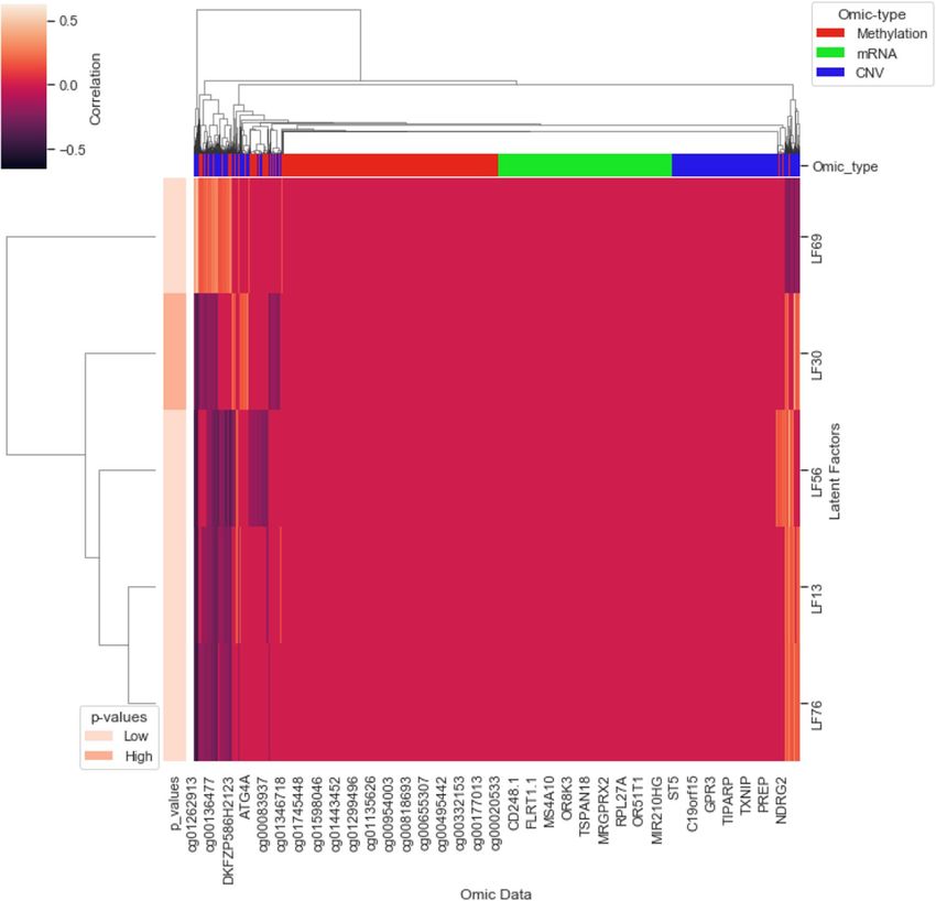
                                            using the same architecture. The implementation presented in Fig. 1 can support unsupervised and supervised
                                            dimensionality reductions. The architecture includes three main components: an encoder, a decoder and a clas-
                                            sifier. For the unsupervised dimensionality reduction, the encoder and the decoder learn latent features from the
                                            input without the classifier’s support. However, we need the classifier for supervised learning of latent features.
                                                Like other deep neural network architectures, VAE has two main hyperparameters: the number of layers
                                            and the number of nodes in each hidden layer. Systematic experimentation is the most reliable way to configure
                                            this ­hyperparameters51. We used the configurations from an existing and related work O    ­ miVAE29 to avoid the
                                            experimentation from scratch. We used the same number of hidden layers as the OmiVAE and ran a few experi-
                                            ments to identify the suitable nodes for the hidden and bottleneck layers. For example, we experimented with the
                                            hidden layer one of the encoder and decoder with 4096 and 2048 nodes. We selected 2048 due to insignificant
                                            performance difference between the two sizes and shorter processing time for 2048 nodes.
                                                The encoder network comprised of an input layer and three hidden layers. The decoder network structure
                                            is the mirror image of the encoder structure. Notably, the encoder and decoder share the necessary bottleneck
                                            layers. We used the architecture for mono-omics, di- and tri-omics data, and the size of the bottleneck layers
                                            is same for all the datasets. However, the other layers’ sizes varied according to the omic count (i.e., mono, di
                                            and tri) and omic data. For example, for mono-omics data, such as mRNA data, the input and output layers are
                                            12,043, and hidden layers sizes are 2048 and 1024. As shown in Fig. 1, multi-omics data were integrated using
                                            an unsupervised parallel integration ­method12. The classifier used a 3-layered fully connected artificial neural
                                            network (ANN) with an input layer with nodes equal to the LFs (32/64/128), a hidden layer with nodes equal to
                                            the half of LFs, and an output layer with nodes equal to the class numbers (e.g., 2 for cancer vs normal samples,
                                            4 for molecular subtypes).
                                                The VAE/MMD-VAE architecture does all the activities illustrated in Fig. 1. In the following, using omic(s)
                                            data, we briefly discuss these activities in the perspective of the encoder, decoder and classifier.

                                            • Encoder: The encoder network using two hidden layers encodes mono-omics data into a 1024 dimensional
                                              vector, di-omics data into two 1024 dimensional vectors and tri-omics data into three 1024 dimensional
                                              vectors. The encoding network for the DNA methylation data is different from the other omics data. For
                                              example, in the first hidden layer, each chromosome related DNA methylation data are encoded into corre-
                                              sponding vectors with 256 dimensions wheres for the others, input data are encoded into a 2048 dimensional
                                              vector. This encoding is to capture the intra-chromosome relationships, and second hidden layer for the
                                              DNA methylation data captures the inter-chromosome relationships. For di- and tri-omics data, the second
                                              hidden layer respectively concatenates two and three 1024 dimensional vectors and produces an encoded
                                              512-dimensional vector. The encoder’s final hidden layer fully connects to two output layers. These two lay-
                                              ers of the size of latent code or features (32/64/128) are part of the bottleneck layers and represent the mean
                                              µ and the standard deviation σ in the Gaussian distribution N(µ, σ ) of the latent variable or feature z given

          Scientific Reports |   (2021) 11:6265 |                https://doi.org/10.1038/s41598-021-85285-4                                                          4

Vol:.(1234567890)
www.nature.com/scientificreports/

                                                                               Encoder                                                                                                        Decoder

                            27,579                                                                                                                                                                                                                     27,579

                               1                            256*23                                                                                                                                                256*23                                   1

                                                                                                                                                                                                                                                                  DNA methyla on
           DNA methyla on
                                                                           1                                                                                                                                          1
                               2                                                                                                                                                                                                                           2
                                                                           2                                                                                                                                          2

                              23                                                                                        32/64/128                                                                                                                         23
                                                                     23                                                                             Latent Features Vector                                           23
                                                                                                                                                    z=µ+

                                                                                                                                                                                              1024
                                                                                                                                                                                                                                                           x

                                                                                       1024
                               x                                           x                                                                                                                                           x
                                                                                                                                     σ               ~ N(0, I)

                                                                                                                                                                                                                                                                  mRNA/RNAseq
           mRNA/RNAseq

                                                                                                                                                                                    or

                                                                                                                                                   32/64/

                                                                                                                                                                                              1024

                                                                                                                                                                                                                     2048

                                                                                                                                                                                                                                                         12,043
                                                                                      1024
                                                                                                                                                             z

                                                                                                                                                    128
                                                                                                                                                                           512
                              12,043

                                                                                                     512
                                                                    2048

                                                                                                                                                                                    or
                                                                                                                                    µ

                                                                                                                                                                                              1024
                                                                                       1024

                                                                                                                                                                                                                     2048
                                                                                                                       32/64/128

                                                                                                                                                                                                                                                                  CNVs
                                                                    2048

                                                                                                                                                    supervised LFs

                                                                                                                                                                                                                                                         24,776
            CNVs
                              24,776

                                                                                                                                                       Used for
                                                                                                                        32/64/128

                                                                                                                                                       learning
                                                                                                       Classifier

                                                                                                                                   2/4

                    Input Layer                                                   Hidden Layers                                                Boleneck Layers                          Hidden Layers                                               Output Layer
                                                                                                                                                     A

                                                                                                  (i) Inferring survival subgroup                                          (ii) Predicng subgroups labels for new samples
                            High-dimensional
                                                                                                   High-dimensional omic(s) data                                                         High-dimensional omic(s) data
                              omic(s) data

                                                                                                                                                                                                                                    DNA methyla on
                                                                                                                                                                                                                     mRNA/RNAseq
                                                          DNA methyla on

                                                                                                                                  DNA methyla on
                                            mRNA/RNAseq

                                                                                                                    mRNA/RNAseq

                                                                                                                                                                                                              CNVs
                                   CNVs

                                                                                                       CNVs

                                                                                                                                                                                                            VVAE/MMD-VAE
                               VVAE/MMD-VAE                                                          VVAE/MMD-VAE

                                                                                                                                                                                                                  Test dataset
                             Latent Features (LFs)                                                   Latent Features (LFs)
                                                                                                                                                                                 Training
                                                                                                                                                                               dataset with                       SVM-based
                                                                                                      Univariate Cox-PH                                                          inferred                          classifier
                                                                                                           models                                                               subgroups
                            2 LFs/128LFs-

                                                                ANN/SVM
                              clustering

                                                                 classifier
                                                                   based
                                based

                                                                                              Inferred survival subgroups                                                                     Predicted survival subgroups
                                                                                                                                                                                                                                                     biomarkers
                                                                                                                                                                                                     Correla on

                                                                                                  (iii) Prognosc biomarkers                                             Omic(s) fetures
                                                                                                                                                                                                                                                      Poten al

                    Clustered/classified Cancer
                                                                                                                                                                                                                        Filtering
                                                                                                                                                                                                      analysis

                        samples, molecular                                                                                                                            Clinically important
                             subtypes                                                                                                                                Latent Features with
                                                                                                                                                                           risk groups
                                               B                                                                                                                           C

                                                                           Figure 1.  Methods: (A) VAE/MMD-VAE architecture consists of an encoder and a decoder made from 3
                                                                           hidden layers and a bottleneck made from 2 layers and a 3-layered ANN-based classifier for supervised LFs
                                                                           learning, (B) Clustering using 2 LFs and ANN-based classification (e.g., cancer vs normal, and molecular
                                                                           subtypes) using 2 and 128 LFs, (C) Survival analysis using 128 LFs: (i) inferring survival subgroup, (ii)
                                                                           predicting subgroup and (iii) potential prognostic biomarkers.

                                                                               input sample x or simply qφ (z|x). As illustrated in Figs. 1 and 7 in Supplementary documents, a reparam-
                                                                               eterisation trick is applied ( z = µ + σ ǫ, where ǫ is a random variable sampled from unit normal distribution

Scientific Reports |                   (2021) 11:6265 |                                           https://doi.org/10.1038/s41598-021-85285-4                                                                                                                                       5

                                                                                                                                                                                                                                                                    Vol.:(0123456789)
www.nature.com/scientificreports/

                                              N(0, I)) in the bottleneck layer to make the sampling process differentiable and suitable for backpropagation.
                                              The sampled latent features vector (z/LFs) is the compressed lower-dimensional representation of omics or
                                              integrated multi-omics data.
                                            • Decoder: The decoder network takes the latent feature vector z as the input and passes through three hidden
                                              layers, and finally outputs the reconstructed vector x ′ of the input omics data. The decoder is also responsible
                                              for estimating the overall loss using Eqs. (4) and (6) respectively for VAE and MMD-VAE.
                                                                         1 M                   c
                                                              LVAE = k                ′
                                                                          � CE(xmj , xm   ) + �c=0            ′
                                                                                                   CE(xomc , xom   ) + LKL                                  (4)
                                                                         M j=1          j                        c

                                                where k is a binary variable set to 1, if there is any DNA methylation data in the input otherwise set to 0, M
                                               is the number of chomosomes, CE is the binary cross-entropy between input data (i.e., xmj - DNA methyla-
                                               tion, xomc - other omic data) and reconstructed data (i.e., xm
                                                                                                            ′ - DNA methylation and x ′
                                                                                                              j                        omc - other omic data),
                                               c = 0, 1, 2 - other omic data count, and LKL is the KL divergence between the learned distribution and a unit
                                               normal distribution N(0, I), which is:
                                                                              LKL =DKL (N(µ, σ ) � N(0, I))                                                 (5)

                                                                           1 M                    c
                                                           LMMD−VAE =k                   ′
                                                                            � nll(xmj , xm   ) + �c=0             ′
                                                                                                      nll(xomc , xom   ) + LMMD                             (6)
                                                                           M j=1           j                         c

                                                where nll- negative log likelihood which can be calculated as mean of (xmj − xm′ )2 for DNA methylation data
                                                                                                                                 j
                                                and mean of (xomc − xom ′ )2 for other omics data, L
                                                                           c                         MMD  is MMD   (Eq.  2) between   the learned distribution
                                                and a unit normal distribution N(0, I), which is:
                                                                           LMMD = MMD(N(µ, σ ) � N(0, I))                                                   (7)
                                                 Classifier: In an unsupervised VAE, the bottleneck layer tends to extract the essential features to reconstruct
                                                input samples as closely as possible. However, these extracted features may not be related to a specific task,
                                                such as a molecular subtype classification. The classifier works as an additional regularisation on top of the
                                                bottleneck layer. With this additional regularisation, the classifier encourages the VAE or MMD-VAE network
                                                to learn LFs that can not only accurately reconstruct the input sample but also, identify cancer and classify
                                                molecular ­subtypes29. The binary cross-entropy based classification loss ( Lcl ) can be added to LMMD−VAE or
                                                LVAE to estimate the total loss using the following Equation:
                                                                                 LVAEtotal = αLVAE + βLcl                                                   (8)
                                                 where α and β are weights of the two losses in the total loss. Equation (8) can be used for the total loss of
                                                MMD-VAE ( LMMD−VAEtotal ) by replacing LVAE with LMMD−VAE . The supervised and unsupervised learning
                                                of LFs depends on the value of β . We use β = 0 for the unsupervised and β = 1 or any positive value for the
                                                supervised learning of LFs.
                                            We used a batch normalisation technique in each fully connected block to implement the VAE/MMD-VAE DL
                                            architecture. This is to address the internal covariate shift (The distribution of the inputs of each layer changes
                                            during training, when previous layers’ parameters change, which slows down the training process.) by nor-
                                            malising layer ­inputs52. Thus, it stabilises the learning process and significantly improves the learning speed.
                                            As the activation function, we used the rectified linear units (ReLU) for the hidden layers, the sigmoid for the
                                            decoder’s output layer and the softmax for classifiers’ output layer. We built the model using PyTorch (version
                                            1.5.0). The implementations of the models used in this paper are available on GitHub (https://github.com/hiraz/
                                            MMD-VAE4Omics).

                                            Clustering and classification in cancer. Cancer samples identification and molecular subtypes are useful in
                                            prognostic and therapeutic stratification of patients and improved management of ­cancers13,25,53. Hence, cor-
                                            rect clustering and classification of ovarian cancer samples and molecular subtypes are important for improved
                                            disease management. Authors ­in13,25,53 have identified four ovarian cancer transcriptional (one molecular sub-
                                            type (We will use transcriptional subtypes and molecular subtypes interchangeably.)) subtypes, which may have
                                            clinical significance. These four subtypes of high grade serous ovarian cancer (HGS-OvCa) are named as Immu-
                                            noreactive, Differentiated, Proliferative and M­ esenchymal13,54. The datasets used in this work are about HGS-
                                            OvCa, and the clinical data include these molecular subtypes for most of the samples. Although these molecular
                                            subtypes are transcriptional (e.g., mRNA), they can be used for other omics data analysis due to their correlation
                                            or association with transcriptional ­data55–58. For example, authors ­in55 have reported that DNA methylation is
                                            often negatively associated with gene expression in promoter regions, while DNA methylation is often positively
                                            associated with gene expression in gene bodies.
                                                VAE or MMD-VAE generated latent and compressed features (z or LFs) can be used to cluster and classify
                                            cancer samples, subtypes, including existing transcriptional or molecular subtypes of ovarian cancer. The per-
                                            formance of clustering and classification exploiting z can demonstrate the dimensionality reduction capability
                                            of VAE or MMD-VAE. We demonstrated the dimensionality reduction capability of VAE and MMD-VAE using
                                            the latent features learned from the mono-omics, integrated di-and tri-omics data of ovarian cancer, and used
                                            for the followings:

          Scientific Reports |   (2021) 11:6265 |                https://doi.org/10.1038/s41598-021-85285-4                                                   6

Vol:.(1234567890)
www.nature.com/scientificreports/

                                  • Clustering We can use the LFs learned (unsupervised and supervised) by the VAE/MMD-VAE models to clus-
                                    ter samples into cancer vs normal and molecular subtypes. We used a two- and three-dimensional embedding
                                    of the mono-omics, di- and tri-omics features for the selected samples, and visualised the clustered samples
                                    using scatter plots. Two dimensional (2D) and three dimensional (3D) embedding of the omic(s) features
                                    for the selected samples are accomplished by selecting first 2 and 3 LFs from the learned LFs (Fig. 1B (left-
                                    side)). We then used the embedded features to cluster the samples into two groups for cancer identification
                                    (cancer and normal samples), and four groups (4 molecular subtypes) for molecular subtypes using 2D and
                                    3D scatter plots.
                                  • Classification We used an ANN-based classifier to classify cancer samples and molecular subtypes using
                                    the LFs learned through the unsupervised process. For all the omics data, we selected the first two and all
                                    LFs learned by VAE/MMD-VAE to classify the samples (Fig. 1B right-side). For the LFs learned through
                                    the supervised process, we used the VAE/MMD-VAE architecture’s classifier to classify the molecular sub-
                                    types. All the classification experiments were validated using a 5-fold cross-validation. In each round of the
                                    validation, 80% data were used for the training, and the rest 20% were left out from the training and used
                                    for separate testing. We presented the classification performances for both classifiers in terms of accuracy,
                                    precision, recall, and f1 score. We also presented a confusion matrix for each classification task done using
                                    the LFs learned through supervised VAE/MMD-VAE models. We have selected the first 2 LFs for the cluster-
                                    ing and classification for simplicity reason. However, one can select any 2 LFs from the learned LFs, and the
                                    performance will be similar to the presented ones.

                                  For the LFs learned using the unsupervised VAE/MMD-VAE models, we compared the clustering and classifica-
                                  tion performances with two popular traditional dimensionality reduction methods, namely PCA and t-SNE59.
                                  We also illustrated how a combination of a traditional method (e.g., t-SNE) and MMD-VAE/VAE performs in
                                  molecular subtypes clustering.

                                  Survival analysis. Identification of robust survival subgroups of ovarian cancer (HGS-OvCa) can significantly
                                  improve patient care. Existing molecular subtypes of HGS-OvCa, such as transcriptional molecular s­ ubtypes13
                                  may not be useful in survival subgroups prediction as most of these studies do the subtyping without relying on
                                  survival data. In this study, first, we used existing transcriptional subtypes for survival analysis and then used
                                  the learned (supervised) LFs inferring and predicting survival subgroups of HGS-OvCa. We followed a 3-step
                                  process (Fig. 1C) as below to do the subgrouping and their corresponding survival analysis:

                                  • Inferring survival subgroup: We built a univariate Cox proportional hazards (Cox-PH) model for each of
                                    the LFs produced by the VAE/MMD-VAE (Fig. 1C(i)). Then, we identified clinically relevant LFs for which a
                                    significant Cox-PH model was found (log-rank p < 0.05). Next, we used these reduced and clinically relevant
                                    LFs (CRLFs) to cluster the samples using a K-means clustering algorithm. We used the R package ­NbClust60
                                     to determine the optimal K value (number of clusters). NbClust can calculate up to 30 indices or metrics to
                                     determine the optimal number of clusters in a data set. It also identifies the best value for K by the majority
                                     rule. In our all 11 datasets (see Table 1), optimal values were between 4 and 2. Considering the small sample
                                    sizes 481 and 292 with a low number of events, we chose K = 2, which means we identified/inferred two
                                     survival subgroups.
                                  • Predicting survival group labels for new samples: After having the survival subgroups labels from K-means
                                    clustering, we used an SVM-based classifier (Fig. 1C(ii)) to predict survival subgroup labels for new samples.
                                     We used a 60%/40% (training/test sets) of all the datasets to have sufficient test samples in most cases that
                                     generate evaluation metrics. We used the tune function of R package e107161 to train the SVM model as it
                                    tunes the model parameters through cross-validation (5-fold) and identify the best model for a training
                                    dataset. In each round of the validation, 60% data were used for training and rest 40% were left out from the
                                    training as the test dataset. Finally, we used the test dataset to predict the survival subgroup or risk labels. We
                                    used the Cox-PH model and Kaplan-Meier (KM) survival curves to evaluate survival prediction performance.
                                    We used the following three metrics for the evaluation:
                                  	 Concordance index The concordance index or C-index is a metric to evaluate the predictions made by an
                                    algorithm. Based on Harrell C ­statistics62, C-index can be defined as the fraction of all pairs of individuals
                                    whose predicted survival times are correctly o   ­ rdered63. The C-index score range between 0 and 1 and a score
                                     around 0.70 indicates a good model, whereas a score around 0.50 means predictions are no better than a
                                     coin flip in determining which patient will live longer. To calculate the C-index, we first built a multi-variate
                                     Cox-PH model using the training set (including the inferred survival subgroup labels and clinical features).
                                     We then predicted survival using the labels of the test set. We then computed the C-index using concordance
                                     function of R’s survival ­package64. Similarly, we calculated the C-index only considering the clinical features
                                    (i.e., status, grade).
                                  	 P value of Cox-PH regression The Cox-PH models built on training datasets compute log-rank p values
                                    for the models. Also, we plotted the Kaplan-Meier survival curves of the two survival subgroups (predicted)
                                    and calculated the log-rank p-value of the survival difference between them.
                                  	 Brier score Brier score function measures the accuracy of probabilistic p        ­ rediction65. In survival analysis,
                                    it measures the mean of the difference between the observed and the estimated survival beyond a certain
                                    ­time66. The score ranges between 0 and 1, and a smaller score indicates better accuracy of the prediction. We
                                    used the R Package survAUC​67 to compute the Brier score.
                                  • Identifying prognostic biomarkers from LFs: We did all the above analyses using the LFs as their compressed
                                    representations simplify the survival analysis and molecular subtyping. However, we need to map these

Scientific Reports |   (2021) 11:6265 |                https://doi.org/10.1038/s41598-021-85285-4                                                      7

                                                                                                                                                  Vol.:(0123456789)
www.nature.com/scientificreports/

                                 (a) Using PCA learned LFs                    (b) Using t-SNE learned LFs                    (c) Using VAE learned LFs

                           (d) Using MMD-VAE learned LFs                   (e) Using VAE+t-SNE learned LFs            (f) Using MMD-VAE+t-SNE learned LFs

                                              Figure 2.  Clustering of normal and cancer samples using the LFs learned using unsupervised PCA, t-SNE,
                                              VAE & MMD-VAE (using 2D for PCA & t-SNE and first 2 LFs for VAE and MMD-VAE) (a)–(d)) on DNA
                                              methylation (mono-omics) data from the GDC cohort. t-SNE was used (e,f) on the 128 learned LFs to identify 2
                                              LFs for the clustering. Legends: 0—Normal, 1—Cancer.

                                                  LFs back to their corresponding input features to identify potential molecular biomarkers. We mapped the
                                                  associated input features for each clinically relevant LF using a linear model and filtered the features with
                                                  zero or insignificant input feature values. Next, we estimated the correlation between the CRLFs and their
                                                  corresponding input features. Finally, we used the filtered correlation data for hierarchical clustering (colour
                                                  map) of LFs and their input features.

                                              Results
                                              We used the developed DL architecture of VAE/MMD-VAE for cancer samples identification, molecular sub-
                                              types clustering and classification, and survival analysis using the TCGA ovarian cancer datasets. The results
                                              demonstrate the performance of the VAE and MMD-VAE in dimensionality reduction and survival analysis.
                                                  We trained and tested the developed VAE and MMD-VAE models with three different bottleneck layers
                                              ( LFs/z = 32, 64, 128) on the preprocessed omics datasets to demonstrate the integrated multi-omics data analy-
                                              sis capability. We implemented the DL model of VAE/MMD-VAE using the network architecture presented in
                                              Fig. 1. We tested the model in unsupervised and supervised settings. We used the Adam optimiser with learning
                                              rate 10−3 due to its superior performance compared to other stochastic optimisation ­methods68. We reported
                                              the results only for LFs/z = 128 due to space limitation and a similar performance pattern. All the classification
                                              performances were cross-validated. Two sets of results were generated, one on cancer samples identification
                                              and molecular subtypes clustering and classification, and another on survival analysis. Importantly, we ran the
                                              experiments on four mono omics, five di-omics and two tri-omics datasets’. We presented the results for only
                                              one for each omics data due to space limitation.

                                              Dimensionality reduction. We have demonstrated the dimensionality reduction capability of the devel-
                                              oped VAE/MMD-VAE by ovarian cancer samples identification, and molecular subtypes clustering and clas-
                                              sification. We also carried out a survival analysis of the TCGA ovarian cancer dataset with the latent features set.

                                              Clustering.

                                                 Cancer vs Normal samples: We used the unsupervised setting of the VAE and MMD-VAE to learn the LFs
                                                 of the DNA methylation data of 886 samples (GDC cohort). We have selected the first 2 LFs of the 128 LFs
                                                 to cluster the samples into two groups (cancer and normal). The two-dimensional embedding of the DNA
                                                 methylation dataset’s input features was plotted on scatter plots for PCA, t-SNE, VAE and MMD-VAE. As
                                                 illustrated in Fig. 2, even with the unsupervised setting, all the dimensionality reduction methods demon-
                                                 strate clustering accuracy over 95%, thanks to the discriminative nature of the input features. MMD-VAE

          Scientific Reports |     (2021) 11:6265 |                https://doi.org/10.1038/s41598-021-85285-4                                                   8

Vol:.(1234567890)
www.nature.com/scientificreports/

                                     outperforms others by correctly clustering 883 samples out of 886. However, the distance between the clusters
                                     is an issue, especially in MMD-VAE, which was improved (shown in Fig. 2e,f) for VAE and MMD-VAE by
                                     combining t-SNE with them. The cancer samples are compact within the cluster (orange dots) compared to the
                                     normal samples. The sub-clusters within the normal samples could be due to the variances within the samples.
                                     Molecular subtypes clustering: We clustered the transcriptional subtypes using the LFs learned through
                                     unsupervised and supervised VAE and MMD-VAE models. For the LFs learned via unsupervised model, we
                                     have selected the first 2 LFs of the learned 128 LFs to cluster the molecular subtypes. The two-dimensional
                                     embedding of the mono omic, di-omics and tri-omics datasets’ input features were plotted on scatter plots
                                     for PCA, t-SNE, VAE and MMD-VAE. Figure 9 in Supplementary documents presents the results of 2
                                     LFs-based molecular subtypes clustering. As seen in Fig. 9b–i in Supplementary documents, all the dimen-
                                     sionality reduction methods poorly clustered the samples into four subtypes using the mono- and tri-omics
                                     datasets. This result is expected as the original omics datasets are not discriminative or well representative
                                     of the transcriptional subtypes. As Fig. 9a in Supplementary documents illustrates, even the most relevant
                                     transcriptional dataset (mRNA) do not represent the transcriptional subtypes. Hence, the unsupervised PCA,
                                     t-SNE, VAE and MMD-VAE models struggle to cluster the transcriptional subtypes. In this context, we can
                                     use the supervised versions of these models, especially VAE and MMD-VAE. We used the supervised VAE
                                     and MMD-VAE models to learn the task-oriented (i.e., the transcriptional subtypes) or guided LFs from
                                     the mono-, di- and tri-omics datasets. We have selected the first 2 LFs of the learned 128 LFs to cluster the
                                     molecular subtypes. Figure 3 presents a part of the clustering results for the supervised VAE and MMD-VAE.
                                     As Fig. 3a–j illustrates, the supervised VAE and MMD-VAE have significantly improved their clustering per-
                                     formance compared to their unsupervised counterparts (Fig. 9 in Supplementary documents) in all omics
                                     datasets. As illustrated in the Figure, the transcriptional (mRNA -mono-omics) dataset is outperforming
                                     other datasets, mainly other mono- omics (i.e., methylation and CNV) datasets, and MMD-VAE outperforms
                                     VAE in most datasets. Also, we have combined the t-SNE with VAE and MMD-VAE, which improve the
                                     performance (shown in Fig. 3k,l compared to their implementations without t-SNE.

                                  Classification.

                                     Cancer samples identification: We used an SVM-based classifier to identify the cancer samples from the
                                     normal samples using the LFs learned through the unsupervised PCA, t-SNE, VAE and MMD-VAE. Table 3
                                     in Supplementary documents presents the classification performances for the DNA methylation dataset of
                                     886 samples (GDC cohort). All the models except t-SNE have more than 99% classification accuracy with
                                     very high precision (0.99), recall (0.99) and f1 score (0.99). The discriminative features (cancer vs normal) of
                                     the DNA methylation data is the main reason for this classification performance. Molecular subtypes clas-
                                     sification: Like the transcriptional subtypes clustering, we used the LFs learned through the unsupervised and
                                     supervised VAE and MMD-VAE models in molecular subtypes classification. For the unsupervised setting,
                                     we also compared the classification performance of the LFs learned through VAE and MMD-VAE with of
                                     the LFs learned through PCA and t-SNE. Table 4 in Supplementary documents presents the classification
                                     performance of an ANN-based classifier utilising the LFs learned via these unsupervised models from mono-,
                                     di- and tri-omics datasets. As we can see from the table, the classifier using the PCA and t-SNE generated
                                     LFs poorly classify the existing transcriptional subtypes in all omics datasets. On the other hand, the classi-
                                     fier using the VAE and MMD-VAE generated LFs can classify the transcriptional subtypes for mono-omics
                                     (mainly mRNA), di- and tri-omics data with higher accuracies in the range of 73.2–81.44%. However, the
                                     performances may not be acceptable in many real-life applications. Lack of discriminative features within the
                                     omics datasets for the transcriptional subtypes is the main reason for the low accuracies. Supervised learning
                                     of the LFs can improve the classification performance. In the supervised setting, VAE or MMD-VAE and
                                     the classifier jointly learn the LFs using the transcriptional subtypes as the supervisory guidance. We trained
                                     the joint models on the mono-, di- and tri-omics datasets and tested the models separately. Table 2 presents
                                     the performances of the molecular subtypes classification in terms of accuracy, precision, recall and f1 score.
                                     Figure 10 in Supplementary documents presents the confusion matrices for few of these classification tasks.
                                     As presented in the table, the molecular subtypes classification performances have significantly improved in
                                     all matrices (i.e., accuracy, precision, recall and f1 score) compared to the unsupervised VAE/MMD-VAE
                                     (Table 4 in Supplementary documents). For example, except the CNV and methylation datasets, MMD-
                                     VAE and VAE respectively show accuracies in the range of 93.2-95.5%, and 87.1-95.7% with high precision,
                                     recall and f1 scores. The performances of the CNV and DNA methylation are not satisfactory as they are not
                                     transcriptional omics data. Even these non-transcriptional datasets, especially the DNA methylation dataset,
                                     show a good classification performance with an accuracy range 72.3–75.2%. This performance could be due to
                                     the association or correlation between the omics ­datasets55–58. For the same reason, the use of integrated non-
                                     transcriptional and transcriptional data helps to maintain a similar performance or improve the performances
                                     of the transcriptional subtypes clustering and classification. For example, the accuracy of MMD-VAE using
                                     mRNA is 93.8%, which has been maintained (93.7%) in case of the integrated CNV-mRNA, and improved to
                                     95.5% in case of the integrated CNV-mRNA-methylation datasets. The confusion matrices in Fig. 10b,d,f in
                                     Supplementary documents for MMD-VAE illustrate similar results. As a dimensionality reduction algorithm,
                                     in majority datasets, MMD-VAE shows better performance compared to VAE. This performance difference
                                     could be due to the MMD-based loss function. We tested the supervised MMD-VAE and VAE on omics
                                     datasets with three different sample sizes (i.e., 292, 459, and 481) to demonstrate our findings’ robustness.
                                     We used the learned LFs to classify the transcriptional subtypes and presented the classification accuracies

Scientific Reports |   (2021) 11:6265 |               https://doi.org/10.1038/s41598-021-85285-4                                                   9

                                                                                                                                              Vol.:(0123456789)
www.nature.com/scientificreports/

                                 (a) VAE on DNA methylation              (b) MMD-VAE on DNA methylation                     (c) VAE on mRNA

                                  (d) MMD-VAE on mRNA                         (e) VAE on CNV-mRNA                     (f) MMD-VAE on CNV-mRNA

                             (g) VAE on mRNA-methylation                (h) MMD-VAE on mRNA-methylation                    (i) VAE on tri-omics

                                 (j) MMD-VAE on tri-omics                    (k) VAE+t-SNE on tri-omics              (l) MMD-VAE+t-SNE on tri-omics

                                               Figure 3.  Clustering molecular subtypes using the LFs learned through the supervised VAE & MMD-VAE +
                                               t-SNE (2D or 2 LFs): (a–c) for MMD-VAE respectively for mono-omics, di-omics and tri-omics data, (d–f) for
                                               MMD-VAE + t-SNE respectively for mono-omics, di-omics and tri-omics data. Legends: 0—Immunoreactive,
                                               1—Differentiated, 2—Proliferative and 3—Mesenchymal.

                                                  in Table 5 in Supplementary documents. As seen in the Table, both VAE and MMD-VAE show robust clas-

          Scientific Reports |      (2021) 11:6265 |              https://doi.org/10.1038/s41598-021-85285-4                                            10

Vol:.(1234567890)
www.nature.com/scientificreports/

                                   Method      Omics_data               Accuracy      Precision      Recall         f1 score
                                   V-VAE       CNV                      58.3 ± 0.3    0.63 ± 0.01    0.58 ± 0.03    0.579 ± 0.03
                                   MMD-VAE     CNV                      54.3 ± 0.31   0.58 ± 0.02    0.54 ± 0.02    0.53 ± 0.03
                                   V-VAE       mRNA                     95.7 ± .5     0.95 ± 0.008   0.95 ± 0.05    0.95 ± 0.006
                                  MMD-VAE      mRNA                     93.8 ± .97    0.93 ± 0.006   0.93 ± 0.005   0.93 ± 0.006
                                  V-VAE        Methylation              72.3 ± .8     0.73 ± 0.02    0.72 ± 0.009   0.71 ± 0.006
                                  MMD-VAE      Methylation              75.2 ± .9     0.75 ± 0.019   0.75 ± 0.018   0.75 ± 0.015
                                  V-VAE        CNV_mRNA                 93.7 ± .27    0.93 ± 0.01    0.93 ± 0.008   0.93 ± 0.007
                                  MMD-VAE      CNV_mRNA                 93.7 ± .37    0.94 ± 0.006   0.93 ± 0.007   0.93 ± 0.007
                                  V-VAE        mRNA_methylation         87.1 ± 1.1    0.87 ± 0.009   0.87 ± 0.008   0.87 ± 0.005
                                  MMD-VAE      mRNA_methylation         93.2 ± .97    0.93 ± 0.02    0.93 ± 0.008   0.93 ± 0.005
                                  V-VAE        CNV_mRNA_methylation     89.4 ± .6     0.89 ± 0.02    0.89 ± 0.006   0.89 ± 0.004
                                  MMD-VAE      CNV_mRNA_methylation     95.5 ± .37    0.95 ± 0.02    0.95 ± 0.008   0.95 ± 0.009

                                  Table 2.  Molecular subtypes classification performances using LFs learned via supervised VAE/MMD-VAE.

                                     sification accuracy for the same omics data with different sample sizes.

                                  The dimensionality reduction performance results of VAE and MMD-VAE in clustering and classification dem-
                                  onstrate the followings:

                                  • in any downstream analysis (e.g., classification) unsupervised dimensionality reduction is useful if the input
                                    dataset is discriminative (e.g., cancer vs normal samples), otherwise supervised dimensionality reduction is
                                    necessary, and
                                  • integrated dimensionality reduction and multi-omics analysis of data may improve or maintain the similar
                                    performance of their mono-omics counterparts exploiting their association, without confounding each other.

                                 Survival analysis. We did a comprehensive survival analysis using eleven datasets, including mono-omics
                                 and multi-omics data, particularly for the samples with existing transcriptional subtypes and inferred survival/
                                 risk groups. Considering the space limitation, we presented a subset but enough of the results (Fig. 4 and Fig. 12,
                                 and Table 7 in Supplementary documents) that significantly represent the performance of VAE and MMD-VAE
                                 in survival analysis. Figure 4a (for 481 samples) and Fig. 11 in Supplementary documents (for 292 samples)
                                 present the Kaplan-Meier survival curves for existing transcriptional subtypes. The subtypes are not clinically
                                 significant or associate with survival of patients/samples (log-rank p > 0.05) (Fig. 4a and Fig. 11 in Supplemen-
                                 tary documents).
                                     For LFs-based survival analysis, we conducted a univariate Cox-PH regression on each of the 128 LFs from
                                 each dataset. We identified 5-22 CRLFs associated with survival. The number of CRLFs is different for each
                                 omics dataset. For example, we found 22 LFs for CNV dataset and only 5 LFs for the integrated CNV, DNA
                                 methylation and mRNA dataset). We did a two-stage survival analysis of the samples (481 and 292) using the
                                 two inferred subgroups. In the first stage, we plotted Kaplan-Meier survival curves for all the samples. As seen
                                 in the Kaplan-Meier survival curves (Fig. 4b–f) of the inferred groups by VAE and MMD-VAE, there is a sig-
                                 nificant survival differences (log-rank p > 0.05) for all the omic(s) data accept the tri-omics (log-rank p = 0.4
                                 is higher than threshold α = 0.05), especially for the VAE. This results could be due to the uninformative LFs
                                 learned by the VAE.
                                     In the second stage, we predicted survival subgroup labels using an SVM-based classifier splitting the samples
                                 into training and test data using a 60/40 split ratio. After predicting survival groups for the test datasets, we ran
                                 two multivariate Cox-PH regressions (one for clinical and one for combined = subgroup + clinical co-variates)
                                 on the training samples, then predicted survival using the labels of the test datasets. For the clinical co-variates,
                                 we considered three clinicopathological characteristics of the considered patients: (i) age at diagnosis, (ii) clinical
                                 or FIGO stage, and (iii) grade. We calculated C-indexes, Brier scores and models’ p-values for the training and
                                 held-out test samples for the multivariate Cox-PH regressions. As seen in Table 7 in Supplementary documents,
                                 the training samples generated moderately high C-indexes in between 0.62 − 0.68, low Brier scores in between
                                 0.17 − 0.19 with significant log-rank p-values < 0.05 of the Cox-PH model. A similar trend is observed for the
                                 held-out datasets with little lower C-indexes (0.60 − 0.66) and little higher Brier scores (0.19 − 0.23) with sig-
                                 nificant log-rank p-values < 0.05 of the Cox-PH model. Importantly, as seen from the Table 7 in Supplementary
                                 documents the performances of VAE and MMD-VAE have been improved in case of combined survival analysis
                                 compared to only clinical variables. This confirm that identified survival subgroup does not confound with
                                 clinicopathological variables, rather it improves the prognosis. Finally, we have plotted Kaplan-Meier survival
                                 curves for the predicted survival group labels. As shown in Fig. 12a–f in Supplementary documents, similar
                                 to Fig. 4b–f, there is a significant survival differences (log-rank p > 0.05) for all the omic(s) between predicted
                                 survival groups for all (presented) omics data. However, few datasets’ p values are higher than the threshold
                                 (0.05). Potential reasons for the higher p values or insignificant differences between the predicted survival groups
                                 for the datasets could be (i) the smaller sample size with few events to identify the differences and (ii) too much
                                 compression may have obscured the clinically relevant features.

Scientific Reports |   (2021) 11:6265 |                https://doi.org/10.1038/s41598-021-85285-4                                                    11

                                                                                                                                                 Vol.:(0123456789)
www.nature.com/scientificreports/

                                                                     Tumour_type + 0 + 1 + 2 + 3                                                                                                             Risk_group + 1 + 2                                                                                                                Risk_group + 1 + 2

                                            1.00     ++ +++                                                                                                               1.00     +++                                                                                                                   1.00     ++
                                                      +++++++++++++++++
                                                                      ++                                                                                                            ++++++++++++++++++
                                                                                                                                                                                            +++++++++++++++                                                                                                         +++++++++++++++++++ +
                                                         ++     ++++ ++++ +
                                                          ++++++++                                                                                                                                                                                                                                                            +++++++++++++
                                                                                                                                                                                                                                                                                                                                           +++ + +++ +
                                                                  ++++ + +++ ++                                                                                                                           + +++
                                                                                                                                                                                                              + ++++                                                                                                                                      ++
                                                                         + + +++++                                                                                                                            ++ ++                                                                                                                           +++++
                                                                             + ++ +++++++ +++                                                                                                                    ++ ++ +++                                                                                                                         +          +
                                                                                           + +++                                                                                                                   ++       +++++                                                                                                                    +++             ++
                                            0.75                                           ++ ++++++                                                                      0.75                                                  +++                                                                      0.75                                            ++++
                                                                                                                                                                                                                                  +++                                                                                                                         +++++++++++
                     Survival probability

                                                                                                                                                   Survival probability

                                                                                                                                                                                                                                                                                  Survival probability
                                                                                       + + + ++ + ++                                                                                                                  + +++
                                                                                                                                                                                                                          ++ +
                                                                                                                                                                                                                                     ++                                                                                                                                 +++++
                                                                                               ++ + ++ ++                                                                                                                                                                                                                                                                   ++++
                                                                                                 +                                                                                                                              ++++ ++++ +                                                                                                                                     ++ ++ ++ +
                                                                                                   ++ ++ + + +++
                                                                                                                     +                                                                                                                                  ++                                                                                                                        ++        ++
                                                                                                                                                                                                                                                         ++++                                                                                                                        +++
                                            0.50                                                        + ++                +++                                           0.50                                                                  ++          +++                                          0.50                                                                            + ++ ++
                                                                                                               +++++++           +                                                                                                                 ++             ++                                                                                                                        ++ +             +++ +
                                                                                                                      ++ +                                                                                                                               +           +++                                                                                                                       +++
                                                                                                                           ++                                                                                                                                ++          +                                                                                                                         +
                                                                                                                                 +
                                                                                                                              ++ +                                                                                                                              + +                                                                                                                                         ++
                                                                                                                                 +                                                                                                                                  +                                                                                                                                         ++
                                            0.25                                                                                                                          0.25                                                                                           +                               0.25                                                                                                      +
                                                       p = 0.19                                                                                                                        p = 0.0048                                                                                                                     p = 0.0042

                                            0.00                                                                                                                          0.00                                                                                                                           0.00
                                                    0            10              20             30               40             50         60                                     0             10             20             30                40             50            60                                  0              10               20               30               40              50            60
                                                                                      Time in months                                                                                                                Time in months                                                                                                                    Time in months

                                                   Number at risk                                                                                                                Number at risk                                                                                                                 Number at risk
                     Tumour_type

                                                                                                                                                   Risk_group

                                                                                                                                                                                                                                                                                  Risk_group
                                              0     106          77              65             54               39             27          19                              1     276          222            192            156            107                71            48                            1     162            130             113               90               73              49            38
                                              1     134         109              92             75               52             28          16
                                              2     135         107              86             67               45             33          23                              2     205          149            114             86                59             37            24                            2     319            241             193              152               93              59            34
                                              3     106          78              63             46               30             20          14
                                                     0           10              20             30               40             50          60                                     0            10             20             30                40             50            60                                   0              10              20               30               40              50            60
                                                                                      Time in months                                                                                                                Time in months                                                                                                                    Time in months

                     (a) Survival analysis using molecular subtypes (b) MMD-VAE (mono-omics) & Subgroups                                                                                                                                                                                                 (c) MMD-VAE (di-omics) & Subgroups

                                                                               Risk_group + 1 + 2                                                                                                            Risk_group + 1 + 2                                                                                                                Risk_group + 1 + 2

                                            1.00     +++
                                                       ++++++++++++++++
                                                                                                                                                                          1.00     + + + + +++ +                                                                                                         1.00     +++++
                                                                                                                                                                                                                                                                                                                              ++++++
                                                                                                                                                                                                                                                                                                                     ++++++++++
                                                                                                                                                                                     ++++++++++
                                                             + +++++++                                                                                                                        ++++++++ +++                                                                                                                         ++++++++++
                                                                        +++++                                                                                                                            ++++ +                                                                                                                               +++++
                                                                             ++++                                                                                                                              ++ + + + +                                                                                                                          +++++
                                                                     ++         + ++                                                                                                                                                                                                                                                                     +++++
                                                                                    +++ +++++                                                                                                                    ++ ++
                                            0.75                                            ++++++                                                                        0.75                                        + ++++                                                                             0.75                                                  +++++++++
                                                                                                                                                                                                                                                                                                                                                                        +++++
                     Survival probability

                                                                                                                                                   Survival probability

                                                                                                                                                                                                                                                                                  Survival probability
                                                                                                  +++++                                                                                                                      ++++                                                                                                                                           +++++
                                                                                                      +++                                                                                                                       ++++                                                                                                                                             ++
                                                                                                         ++
                                                                                                              ++++                                                                                                                     +                                                                                                                           +                ++++
                                                                                                     +            +++                                                                                                                      ++                           ++   +                                                                                             +            +++
                                                                                                                      ++                                                                                                                        ++                                                                                                                                          ++ +
                                            0.50                                                                           +++                                            0.50                                                                                                                           0.50                                                                                  ++++
                                                                                                                              ++++                                                                                                                      +++                                                                                                                                        ++
                                                                                                                                 +++                                                                                                                       +                                                                                                                                         ++
                                                                                                                                     + +                                                                                                                                                                                                                                                                  + +
                                                                                                                                        +++                                                                                                                         +                                                                                                                                        +++
                                                                                                                                          ++ +                                                                                                                           ++                                                                                                                                    ++ +
                                                                                                                                                                                                                                                                                                                                                                                                   +
                                                                                                                                                                                                                                                                           ++
                                            0.25                                                                                                                          0.25                                                                                                                           0.25
                                                         p = 0.021                                                                                                                     p = 0.02                                                                                                                       p = 0.4

                                            0.00                                                                                                                          0.00                                                                                                                           0.00
                                                    0            10              20             30               40             50         60                                     0             10             20             30                40             50            60                                  0              10               20               30               40              50            60
                                                                                      Time in months                                                                                                                Time in months                                                                                                                    Time in months

                                                   Number at risk                                                                                                                Number at risk                                                                                                                 Number at risk
                     Risk_group

                                                                                                                                                   Risk_group

                                              1     11           8                4              4                1              0          0                               1     32            23             21             15                14             11            8    Risk_group               1     27              18              14               10                6               4              4
                                              2     470         363             302            238              165            108          72                              2     260          193            157            124                82             55            33                            2     454            353             292              232              160              104           68
                                                     0           10              20             30               40             50          60                                     0            10             20             30                40             50            60                                   0              10              20               30               40              50            60
                                                                                      Time in months                                                                                                                Time in months                                                                                                                    Time in months

                                                   (d) VAE (di-omics) & Risk Groups                                                                                       (e) MMD-VAE (tri-omics) & Subgroups                                                                                                    (f) VAE (tri-omics) & Subgroups

                                                                                           Figure 4.  Survival analysis using existing using molecular subtypes and CRLFs-based survival subgroups:
                                                                                           (a) survival analysis using the existing transcriptional subtypes show that they are not linked to the survival
                                                                                           ( p = 0.19 < 0.05), (b–f) survival analysis using the two subgroups show significant survival differences
                                                                                           ( p < 0.05) between the groups. The results in (e) for 292 samples, and the rest are for 481 samples.

                                                                                              From Fig. 4b–f and Fig. 12 and Table 7 in Supplementary documents we have the following two key
                                                                                           observations:

                                                                                           • Impact of inferred subgroups on survival: In case of mono-omics and multi-omics data, inferred subgroups
                                                                                             combined with the clinical covariates (i.e., stage, grade and age) improve the survival prediction. For example,
                                                                                             subgroups learned using the MMD-VAE on CNV mono-omics data combined with clinical features shows
                                                                                             higher C-index value (0.63) than the C-index value (0.62) for the clinical features. However, the improvement
                                                                                             is not that significant. In summary, inferred subgroups, combined with the clinical features, demonstrate
                                                                                             survival prediction performance higher than or similar to the clinical features.
                                                                                           • mono-omics vs multi-omics based LFs in survival: Similar to molecular subtypes classification, multi-omics
                                                                                             based LFs may incrementally (e.g., di- and tri-omics) improve the survival subgroups classification accuracy
                                                                                             compared to mono-omics based LFs (shown in Table 6 in Supplementary documents). However, multi-omics
                                                                                             (i.e., CNV_mRNA, CNV_mRNA_methylation) based LFs and subgroups predicted based on them do not
                                                                                             improve the survival prediction performances than their mono-omics counterparts. Potential reasons for
                                                                                             the lower performance using multi-omics based LFs could be due to (i) smaller sample size with few events
                                                                                             (e.g., 143 out of 292 samples) to identify the differences, (ii) too much compression (e.g., for CNV + DNA
                                                                                             methylation + mRNA data 64,398 input features to 128 LFs) may have obscured the clinically relevant fea-
                                                                                             tures.

                                                                                           Finally, we presented a simple method to identify potential prognostic biomarkers from the clinically relevant LFs
                                                                                           using a linear model. Figure 5 presents the association between the CRLFs and the input features for tri-omics
                                                                                           (CNV_mRNA_methylation) data. For example, our mapping has identified the NDRG2 gene as a potential

          Scientific Reports |                                 (2021) 11:6265 |                                                                  https://doi.org/10.1038/s41598-021-85285-4                                                                                                                                                                                                                        12

Vol:.(1234567890)
You can also read