Statistical Downscaling of Precipitation and Temperature Using Long Ashton Research Station Weather Generator in Zambia: A Case of Mount Makulu ...
←
→
Page content transcription
If your browser does not render page correctly, please read the page content below
American Journal of Climate Change, 2017, 6, 487-512
                                                                                                http://www.scirp.org/journal/ajcc
                                                                                                          ISSN Online: 2167-9509
                                                                                                            ISSN Print: 2167-9495

Statistical Downscaling of Precipitation and
Temperature Using Long Ashton Research
Station Weather Generator in Zambia: A Case
of Mount Makulu Agriculture Research Station

Charles Bwalya Chisanga1,2*, Elijah Phiri2, Vernon R. N. Chinene2

Ministry of Agriculture, Ndola, Zambia
1

Department of Soil Science, School of Agricultural Sciences, University of Zambia, Lusaka, Zambia
2

How to cite this paper: Chisanga, C.B.,        Abstract
Phiri, E. and Chinene, V.R.N. (2017) Statis-
tical Downscaling of Precipitation and Tem-    The Long Ashton Research Station Weather Generator (LARS-WG) is a stochas-
perature Using Long Ashton Research Sta-       tic weather generator used for the simulation of weather data at a single site
tion Weather Generator in Zambia: A Case
                                               under both current and future climate conditions using General Circulation
of Mount Makulu Agriculture Research
Station. American Journal of Climate Change,   Models (GCM). It was calibrated using the baseline (1981-2010) and evaluated
6, 487-512.                                    to determine its suitability in generating synthetic weather data for 2020 and
https://doi.org/10.4236/ajcc.2017.63025        2055 according to the projections of HadCM3 and BCCR-BCM2 GCMs under
Received: April 12, 2017
                                               SRB1 and SRA1B scenarios at Mount Makulu (Latitude: 15.550˚S, Longitude:
Accepted: August 21, 2017                      28.250˚E, Elevation: 1213 meter), Zambia. Three weather parameters—preci-
Published: August 24, 2017                     pitation, minimum and maximum temperature were simulated using LARS-WG
                                               v5.5 for observed station and AgMERRA reanalysis data for Mount Makulu.
Copyright © 2017 by authors and
Scientific Research Publishing Inc.            Monthly means and variances of observed and generated daily precipitation,
This work is licensed under the Creative       maximum temperature and minimum temperature were used to evaluate the
Commons Attribution International              suitability of LARS-WG. Other climatic conditions such as wet and dry spells,
License (CC BY 4.0).
http://creativecommons.org/licenses/by/4.0/
                                               seasonal frost and heat spells distributions were also used to assess the per-
                Open Access                    formance of the model. The results showed that these variables were modeled
                                               with good accuracy and LARS-WG could be used with high confidence to re-
                                               produce the current and future climate scenarios. Mount Makulu did not ex-
                                               perience any seasonal frost. The average temperatures for the baseline (Ob-
                                               served station data: 1981-2010 and AgMERRA reanalysis: 1981-2010) were
                                               21.33˚C and 22.21˚C, respectively. Using the observed station data, the average
                                               temperature under SRB1 (2020), SRA1B (2020), SRB1 (2055), SRA1B (2055)
                                               would be 21.90˚C, 21.94˚C, 22.83˚C and 23.18˚C, respectively. Under the Ag-
                                               MERRA reanalysis, the average temperatures would be 22.75˚C (SRB1: 2020),

DOI: 10.4236/ajcc.2017.63025 Aug. 24, 2017                       487                         American Journal of Climate Change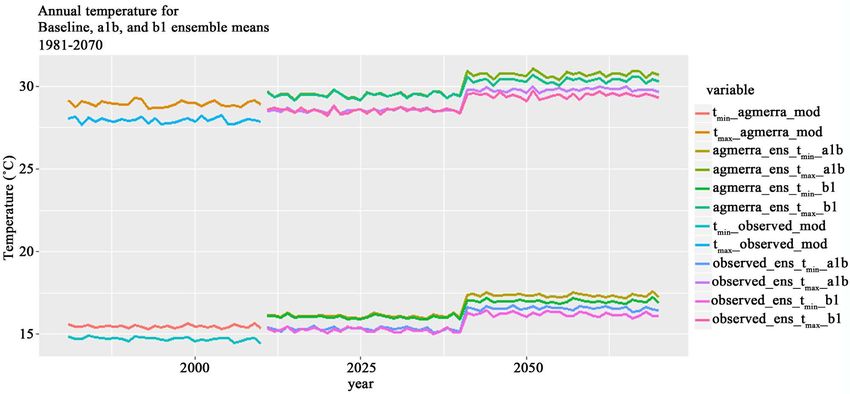
C. B. Chisanga et al.

                                 22.80˚C (SRA1B: 2020), 23.69˚C (SRB1: 2055) and 24.05˚C (SRA1B: 2055). The
                                 HadCM3 and BCM2 GCMs ensemble mean showed that the number of days
                                 with precipitation would increase while the mean precipitation amount in 2020s
                                 and 2050s under SRA1B would reduce by 6.19% to 6.65%. Precipitation would
                                 increase under SRB1 (Observed), SRA1B, and SRB1 (AgMERRA) from 0.31%
                                 to 5.2% in 2020s and 2055s, respectively.

                                 Keywords
                                 LARS-WG, Statistical Downscaling, Climate Change Scenarios,
                                 HadCM3, BCCR-BCM2, GCMs

                               1. Introduction
                               Global Climate Models (GCMs) from Intergovernmental Panel on Climate Change
                               (IPCC) Third and Fifth Coupled Model Inter-comparison Projects (CMIP3 and
                               CMIP5) are tools used to simulate the current and future climate change (maxi-
                               mum and minimum temperature, precipitation, solar radiation, surface pressure,
                               wind, relative, and specific humidity, geopotential height, etc.) of the earth un-
                               der different climate change scenarios [1] [2] [3] [4] due to increasing green-
                               house gases (GHGs). The GHG emissions scenarios reflect the uncertainty of the
                               future climate and GCMs’ striving to represent complex natural systems [5]. The
                               A1B and B1 represents future scenarios of new, and efficient technologies and
                               ecologically friendly, respectively [5]. The IPCC defines a GCM as a numerical
                               (quantitative) representation of the climate system based on the physical, chemi-
                               cal and biological properties of its components, their interactions and feedback
                               processes [6], [7]. GCMs play important roles in advancing the scientific under-
                               standing of large-scale climate variability and trend [8]. The GCMs focus mostly
                               on changes associated with temperature and precipitation [9]. The GCMs depict
                               the climate using a three-dimensional grid over the globe having a horizontal
                               resolution of, between 250 and 600 km, 10 to 20 vertical layers in the atmosphere
                               and sometimes as many as 30 layers in the oceans [3]. Due to the coarse spatial
                               resolution of GCMs, they cannot be used at local or regional scale for impact
                               studies, hence there is need to bridge the gap between the large scale variables
                               (predictors) and local scale variables (predictands).
                                 The methods used to convert the coarse spatial resolution of GCM outputs
                               into high-spatial resolution of point data [10] are usually referred to as down-
                               scaling techniques. There are three available broad approaches to downscaling:
                               1) dynamics [9] [11] [12] [13] [14]; 2) statistics [15] [16]; and 3) hybrid (dynam-
                               ics-statistics) [17] [18]. All statistical downscaling methods are classified according
                               to three sub-groups [19] [20] namely: 1) Transfer Functions (Regression Mod-
                               els); 2) Synoptic Weather Typing (Weather Classification); and 3) Stochastic
                               Weather Generators [21]. Statistical downscaling technique derives statistical re-

DOI: 10.4236/ajcc.2017.63025                         488                          American Journal of Climate Change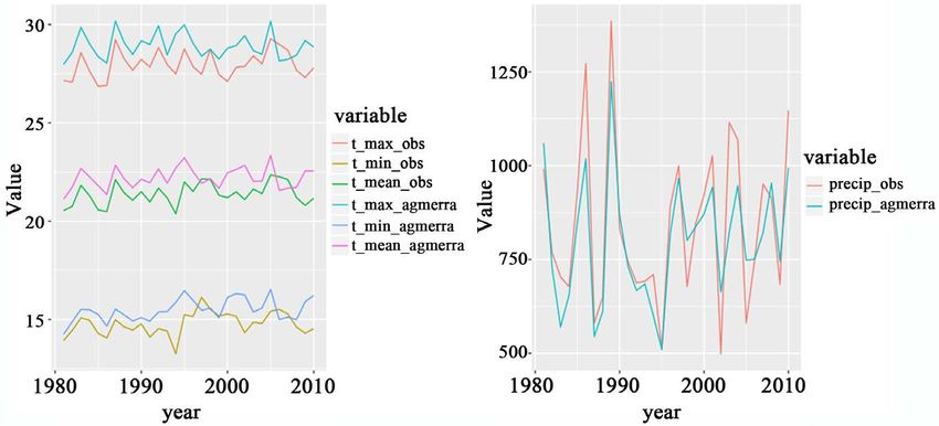
C. B. Chisanga et al.

                               lationships between observed small-scale variables (predictands) and larger (GCM)
                               scale variables (predictors), using either analogue methods, regression analysis or
                               neural network methods [21] [22]. Stochastic weather generators are used in cli-
                               mate change impact studies as computationally inexpensive tool for generating
                               site-specific climate scenarios at a daily time-step with high spatial and temporal
                               resolutions based on GCM outputs [23] [24] [25].
                                 A stochastic weather generator is a computer algorithm that uses existing me-
                               teorological records to produce a long series of synthetic daily weather data of
                               unlimited length for a location based on the statistical characteristics of ob-
                               served weather data at that location [3] [26] [27] [28]. Stochastic weather ge-
                               nerators constitute one of the techniques for developing local scale future cli-
                               mate scenarios from large-scale climate changes simulated by GCMs [29]. It
                               should be understood that stochastic weather generators are not predictive
                               tools, which can be used in weather forecasting, but are a means of generating
                               time-series of synthetic weather that is statistically “identical” to the observed
                               historical weather data [26]. The generated synthetic daily weather data may
                               be used in crop simulation modelling or replace the long-term series of historical
                               data, especially if some data sets are missing or contain erroneous data [30]. In
                               recent years, synthetic weather data generated by weather generators have
                               been used extensively in climate change and variability studies to determine
                               the potential impact on agricultural or hydrological applications [31] [32] [33]
                               [34].
                                 Agricultural productivity is sensitive to direct and indirect effects from changes
                               in temperature, GHG concentration, and precipitation and in soil moisture and
                               the distribution and frequency of infestation by pests and diseases, respectively.
                               Predicted climate change scenarios may affect crop yield, growth rates, photo-
                               synthesis and transpiration rates, soil moisture availability, through changes of
                               water use and agricultural inputs such as herbicides, pesticides, insecticides and
                               fertilizers [35] [36]. [36] reported that the anticipated potential agricultural im-
                               pacts of the simulated climate change include extreme weather condition (drought
                               and floods), soil water management and soil moisture regime. To this end, there
                               is need for farmers to adopt water use efficiency technologies that reduces sur-
                               face evaporation, surface runoff, and increases water storage capacity of the
                               soil.
                                 Stochastic weather generators are conventionally developed in two steps [3]
                               [27]: 1) the first step is to model daily precipitation; and 2) the second step is to
                               model the remaining variables of interest such as daily temperature, solar radia-
                               tion, humidity and wind speed conditional on precipitation occurrence. Differ-
                               ent model parameters are usually required for each month to reflect seasonal
                               variations both in the values of the variables themselves and in their cross-cor-
                               relations. Stochastic downscaling approaches involve modifying the parameters
                               of conventional weather generator such as Weather Generator (WGEN) and Long
                               Ashton Research Station Weather Generator (LARS-WG). Of the available statis-

DOI: 10.4236/ajcc.2017.63025                        489                          American Journal of Climate Change
C. B. Chisanga et al.
tical downscaling techniques, LARS-WG is preferred as it can be used for the
simulation of weather data at a single site [33] based on as little as a single year
of historical data [26] [32] [37] [38] under both current and future climate con-
ditions. The data is in the form of daily time-series for precipitation, tempera-
ture and solar radiation variables. A recent study showed that LARS-WG per-
forms well and has been well validated in diverse climates around the world [32]
[39]. The current LARS-WG version 5.5 includes fifteen (15) GCMs outputs used
in CMIP3 IPCC emission scenarios SRA1B, SRA2 and SRB1 which can be used
in an ensemble to cope with the GCMs uncertainties.
The LARS-WG version 5.5 also improves simulation of extreme weather events,
such as extreme daily precipitation, long dry spells and heat waves [40] [41]. Fu-
ture climate scenarios incorporate changes in climatic variability as well as changes
in mean climate [42]. LARS-WG has not been parameterized and tested in Zam-
bia to be used in generating current and future climate scenarios from GCMs
outputs for impact studies. Reliable data and analysis of temperature and preci-
pitation evolution is an important aspect in generating current and future cli-
mate scenarios. If a weather generator is adequately calibrated and validated in
simulating the mean as well as extreme properties of temperature and precipita-
tion (wet/dry spell length and annual maximum rainfall) it can be adopted as a
simplified, computationally inexpensive local solution for incorporating climate
change information into decision support systems [41]. The objectives of this
study were: to assess the suitability of LARS-WG in predicting climate change
for 2020s and 2055s according to the projections of HadCM3 and BCCR-BCM2
GCMs for B1 and A1B scenarios.
2. Materials and Methods
2.1. Study Site
The study site was Mount Makulu Research Station in Chilanga (Latitude: 15.550˚S,
Longitude: 28.250˚E, Elevation: 1213 meter). The Region receives between 800 to
1000 mm of annual rainfall. The climate at the site is described as a wet and dry
tropical and sub-tropical and is modified by altitude [43].
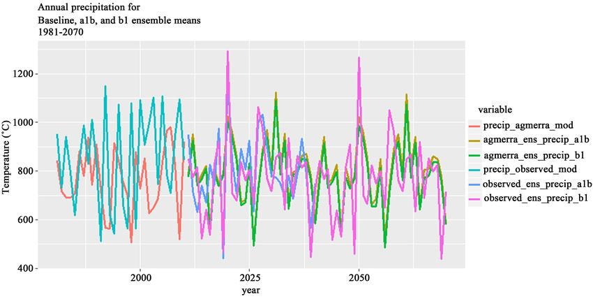
2.2. Weather Data
Historical climate data for daily rainfall (precip), minimum (Tmin) and maxi-
mum (Tmax) air temperature was obtained from the Zambia Meteorological
Department (ZMD) for the period 1981-2010 and the Agricultural Modern-Era
Retrospective Analysis for Research and Applications (AgMERRA) Climate
Forcing Dataset for Agricultural Modeling for the period 1981-2010 [44] (Figure
1). The weather data from ZMD data did not include solar radiation. 5.39%,
4.39% and 1.95% of the Tmin, Tmax and precipitation data was missing from
the observed station data. On the other hand, the AgMERRA datasets are stored
at 0.25˚ × 0.25˚ horizontal resolution (~25 km), with global coverage and daily
DOI: 10.4236/ajcc.2017.63025 490 American Journal of Climate ChangeC. B. Chisanga et al.
Figure 1. Observed station and AgMERRA reanalysis data for precipitation and temper-
ature.
values from 1980-2010 in order to form a “baseline or current period” climato-
logy [44]. The AgMERRA reanalysis data was collected from AgMERRA Climate
Forcing Dataset for Agricultural Modeling
(https://data.giss.nasa.gov/impacts/agmipcf/agmerra/).
2.3. General Circulation Models
The Hadley Centre Couple Model version 3 (HadCM3) and Bergen Climate Mod-
el Version 2 (BCCR-BCM2) models were used in the IPCC Third and Fourth As-
sessments and also contributed to the Fifth Assessment Reports [45]. These two
models differ in spatial resolution power, design institute, predictability of at-
mospheric variables, and predictability of oceanic variables [46] [47]. The ocea-
nic component of HadCM3 has a horizontal resolution of 1.25˚ × 1.25˚ and com-
prises 20 levels. The HadCM3 GCM is ranked highly (fourth out of 22 CMIP3
models) when compared with other GCMs. The simulation of HadCM3 assumes
the year length in 360 day calendar with 30 days per month [48]. The model was
developed in 1999 and was the first coupled atmosphere-ocean which did not re-
quire flux adjustments [49]. It also has the capability to capture the time-dependent
fingerprint of historical climate change in response to natural and anthropogenic
forcings [45] and this has made it an important tool in studies concerning the
detection and attribution of past climate changes.
The Bergen Climate Model Version 2 (BCCR-BCM2) is a fully-coupled atmos-
phere-ocean-sea-ice model that provides state-of-the-art computer simulations
of the present and future climate scenarios [50]. It is deployed at Bjerknes Centre
for Climate Research (Norway) Computer. The model has oceanic resolution
[1.5˚ × 1.5˚ (0.5˚) L35] of 35 vertical layers and approximately square horizontal
grid cells with 1.5˚ grid spacing along the equator [51] [52]. Near the equator the
meridional grid spacing is gradually decreased to 0.5˚. It has a triangular trunca-
tion T63 with “linear” reduced Gaussian grid equivalent to T42 quadratic grid
(2.8˚) [53].
DOI: 10.4236/ajcc.2017.63025 491 American Journal of Climate ChangeC. B. Chisanga et al.
2.4. Description of LARS-WG Stochastic Weather Generator Model
The Long Ashton Research Station Weather Generator (LARS-WG) is a stochas-
tic weather generator [38] used for the simulation of weather data at a single site
[33], under both current and future climate conditions. The data required by the
weather generator is in the form of daily time-series for precipitation (mm),
maximum and minimum temperature (˚C) and solar radiation (MJ·m−2·day−1)
variables. LARS-WG accepts sunshine hours as an alternative to solar radiation
data. If solar radiation data are unavailable, then sunshine hours are used to es-
timate solar radiation using the approach described in [54].
LARS-WG as a stochastic weather generator utilizes a semi empirical distribu-
tion (SED) which is specified as the cumulative probability distribution function
(CPDF) [55] to approximate probability distribution of dry and wet series of
daily precipitation, minimum, and maximum temperature and daily solar radia-
tion [33] [48]. The number of intervals (n) used in SED is 23 for climate variable
[48] compared with ten (10) used in the previous versions. LARS-WG simulates
time-series of daily weather data at a single site “statistically” identical to the ob-
served data and can be used to: 1) generate long-term time-series weather data
suitable for risk assessment in agricultural and hydrological studies; 2) provide
the means of extending the simulation of weather data to unobserved locations;
and 3) serve as a computationally inexpensive tool to produce daily site-specific
climate change scenarios based on outputs from general (global) and regional cli-
mate models for impact assessments of climate change. LARS-WG produces syn-
thetic daily time series of maximum and minimum temperature, precipitation
and solar radiation [56].
2.5. Weather Generation Process and Testing Performance
The process of generating local-scale daily climate scenario data in LARS-WG is
divided into two steps of analysis and generator and briefly described by [33]
and [57] (Figure 2). The baseline data [observed station data (1981-2010) and
AgMERRA reanalysis (1981-2010)] were used to perform site analysis and gen-
eration of synthetic time series data using LARS-WG for HadCM3 and BCCR-
BCM2 GCMs under B1 and A1B scenarios.
Analysis (site analysis and model calibration): Observed daily and AgMERRA
reanalysis weather data for the site were analyzed to compute site parameters
and these were stored in two files: a wgx-file (site parameters file) and a stx-file
(additional statistics), respectively.
Generator (generation of synthetic weather data or site scenarios): the site pa-
rameter files derived from observed daily weather data was used to generate
synthetic daily time series which statistically resembles the observed weather.
The synthetic data corresponding to a particular climate change scenario may
also be generated by applying global climate model-derived changes in precipita-
tion, temperature and solar radiation to the LARS-WG parameter file [33] [57].
Statistical tests used in this study included the Kolmogorov-Simirnov (K-S) test
DOI: 10.4236/ajcc.2017.63025 492 American Journal of Climate ChangeC. B. Chisanga et al.
Figure 2. Systematic structure of downscaling weather data in LARS-WG.
to compare the probability distributions, T-test to compare means and F-test to
compare standard deviations. The statistical tests used in LARS-WG v5.5 are based
on the assumption that the observed/AgMERRA and synthetic weather data are
both random samples from existing distributions and they test the null hypothe-
sis that the two distributions are the same. The LARS-WG was validated by com-
paring statistics computed from a synthetic weather series generated by the weather
generator against those from observed time series weather data [58].
The annual means of precipitation and temperature were computed using en-
sembles under SRA1B and SRB1 scenarios. If the calculated mean annual tem-
perature and precipitation amounts (mm year-1) were within the 95% confidence
interval (CI95) for the synthetic data, it was concluded that the statistic were si-
mulated accurately for Mt. Makulu.
2.5.1. Generation of Climate Scenarios with LARS-WG
Use of at least 20 - 35 years of daily observed weather data is recommended to
determine robust statistical parameters [33] [59] [60]. On the other hand, to model
low frequency, high magnitude events, it is desirable to obtain the longest possible
observed time series [34] [61]. A long record of observations could possibly con-
tain the full variability of the observed climate and hence allow the downscaling
models to better model climate changes [34]. LARS-WG version 5.5 used in this
study incorporates climate scenarios based on 15 GCMs used in IPCC 4th As-
sessment Report (2007) to better deal with uncertainties of GCMs and in this
DOI: 10.4236/ajcc.2017.63025 493 American Journal of Climate ChangeC. B. Chisanga et al.
study two GCMs were used. This version of LARS-WG also improves simula-
tion of extreme weather events such as extreme daily precipitation, duration of
wet/dry spells and heat waves [57]. The extreme properties of rainfall were ana-
lyzed in LARS-WG using baseline data (1981-2010 and 1981-2010) for Mount
Makulu.
The calibrated LARS-WG stochastic weather generator was used to generate
30 years of synthetic daily precipitation, minimum and maximum temperature
for Mount Makulu for the time slice 2011-2030 [near future (2020)] and 2046-
2065 [medium future (2055)] based on the SRB1 and SRA1B from HadCM3 and
BCR2 GCMs for the study site (see Table 1). In LARS-WG model, the GCMs va-
riables are not directly applied, but the model apply the proportionally local sta-
tion climate variables, which are adjusted to the present climate change [62].
2.5.2. Modeling Precipitation Occurrence
According to [57] [63] the simulation of precipitation occurrence is modelled as
alternate wet and dry series, where a wet day is defined to be a day with precipi-
tation > 0.0 mm. The length of each series is chosen randomly from the wet or
dry semi-empirical distribution for the month in which the series starts. In de-
termining the distributions, observed series are also allocated to the month in
which they start. For a wet day, the precipitation value is generated from the
semi-empirical precipitation distribution for the particular month independent
of the length of the wet series or the amount of precipitation on previous days.
For each climatic variable v, a value of a climatic variable vi corresponding to the
probability pi is calculated [16] [57] as in Equation (1):
=vi min {v : P ( vobs ≤ =
v ) ≥ pi } , i 0, , 23 (1)
Table 1. CO2 concentrations (ppm) for selected climate scenarios specified in the Special
Report on Emissions Scenarios (SRES) [46] [68].
CO2 concentration
Scenario Key assumption
2011-2030 2046-2065 2081-2100
Population convergence
B1
throughout the world, change in
(“low” GHG
economic structure (pollutant 410 492 538
emission
reduction and introduction to
scenario”)
clean technology resources).
Rapid economic growth,
A1B (“medium”
maximum population growth
GHG
during half century and after that 418 541 674
emission
decreasing trend, rapid modern
scenario)
and effective technology growth.
Rapid world population growth,
A2 (“high”
heterogeneous economics in
GHG emission 414 545 754
direction of regional conditions
scenario)
throughout the world.
Note: CO2 concentration for the baseline scenario, 1960-1990, is 334 ppm.
DOI: 10.4236/ajcc.2017.63025 494 American Journal of Climate ChangeC. B. Chisanga et al.
where P() denotes probability based on observed data {vobs}. For each climatic
variable, two values, p0 and pn, are fixed as p0 = 0 and pn = 1, with corresponding
values of v0 = min{vobs} and vn = max{vobs}. To approximate the extreme values of
a climatic variable accurately, some pi are assigned close to 0 for extremely low
values of the variable and close to 1 for extremely high values and the remaining
values of pi are distributed evenly on the probability scale. Because the probabil-
ity of very low daily precipitation (C. B. Chisanga et al.
the behavior of the pair (X, Y). A joint distribution of two random variables has
a probability density function f(x, y) that is a function of two variables (some-
times denoted fx,y(x, y)). The joint behavior of X and Y is fully captured in the
joint probability distribution. If X and Y are continuous random variables, then
f(x, y) must satisfy the equation below:
∞
1) E X mY n = ∫ ∫ x m y n f XY ( x, y ) dxdy (3)
−∞
or
∞ ∞
2) f ( x, y ) ≥ 0 and ∫ ∫ f ( x, y ) dydx =
1 (4)
−∞ −∞
If X and Y are discrete random variables, then f(x, y) must satisfy the equa-
tions below:
1) E X mY n = ∑ x∈S ∑ y∈S x m y n P ( x, y ) (5)
x y
or
2) 0 ≤ f ( x, y ) ≤ 1 and ∑ x ∑ y f ( x, y ) =
1 (6)
The Joint PDF Estimator developed by [64] was used to compute the JPDF for
the observed and AgMERRA data. The application was written in Java and reads
CSV files. The application estimates JPDFs from sample data, by transforming a
set of random variables into a set of independent ones and by computing the
marginal PDFs of the latter [64].
3. Results and Discussion
3.1. Calibration and Validation LARS-WG Results
The Calibration and validation was carried out using the “Site Analysis” and
“Qtest” function in LARS-WG model using two data sets, Observed station and
AgMERRA reanalysis data, respectively. Performance of the weather genera-
tor during the calibration and the validation was checked using Kolmogo-
rov-Simirnov (K-S) test, T-test and the F-test. The performance was also checked
by using coefficient of correlation (R) and coefficient of determinant (R2). Eva-
luating the suitability of LARS-WG performance in simulating precipitation for
Mount Makulu is presented in Table 2 and Table 3. It can be observed from the
K-S-test that the model performed very well in fitting the DJF (wet/dry), MAM
(wet/dry), JJA (wet) and SON (dry) seasons for the two datasets. [63] and [65]
reported that LARS-WG was more capable in simulating the seasonal distribu-
tions of the wet/dry spells and the daily precipitation distributions in each month.
The model performed poorly in fitting the JJA (dry) season. The reason for the
poor performance is attributed to lack of precipitation recorded in JJA (dry).
Table 4 and Table 5 present the KS-test for daily rain distribution. The assess-
ment results show that LARS-WG performance in simulating daily rainfall
distributions for the JFMAOND was perfect except for the months of MJJAS
(Observed) and MJJAS (AgMERRA reanalysis). The poor performance was due
DOI: 10.4236/ajcc.2017.63025 496 American Journal of Climate ChangeC. B. Chisanga et al.
Table 2. K-S-test for seasonal wet/dry SERIES distribution for AgMERRA data.
Season Wet/dry N K-S p -value Assessment
DJF wet 12 0.049 1.0000 Perfect fit
DJF dry 12 0.045 1.0000 Perfect fit
MAM wet 12 0.077 1.0000 Perfect fit
MAM dry 12 0.075 1.0000 Perfect fit
JJA wet 12 0.000 1.0000 Perfect fit
JJA dry 12 0.131 0.9824 Very good fit
SON wet 12 0.079 1.0000 Very good fit
SON dry 12 0.098 0.9997 Perfect fit
Table 3. K-S-test for seasonal wet/dry SERIES distribution for observed data.
Season Wet/dry N K-S p -value Assessment
DJF wet 12 0.030 1.0000 Perfect fit
DJF dry 12 0.193 0.7751 Perfect fit
MAM wet 12 0.034 1.0000 Perfect fit
MAM dry 12 0.175 0.8366 Perfect fit
JJA wet 12 0.000 1.0000 Perfect fit
JJA dry 12 1.000 0.0000 Very poor fit
SON wet 12 0.070 1.0000 Very good fit
SON dry 12 0.135 0.9761 Perfect fit
Table 4. KS-test for daily RAIN distributions for AgMERRA data.
Month N K-S p -value Assessment
J 12 0.073 1.0000 Perfect fit
F 12 0.068 1.0000 Perfect fit
M 12 0.121 0.9929 Perfect fit
A 12 0.099 0.9997 Perfect fit
M 12 0.206 0.6609 Good fit
J 12 0.261 0.3593 Very poor fit
J 12 0.566 0.0006 Very poor fit
A 12 0.348 0.0955 Very poor fit
S 12 0.305 0.1932 Very poor fit
O 12 0.092 1.0000 Perfect fit
N 12 0.170 0.8611 Perfect fit
D 12 0.068 1.0000 Perfect fit
DOI: 10.4236/ajcc.2017.63025 497 American Journal of Climate ChangeC. B. Chisanga et al.
Table 5. KS-test for daily RAIN distributions for station observed data.
Month N K-S p -value Assessment
J 12 0.132 0.9809 Perfect fit
F 12 0.052 1.0000 Perfect fit
M 12 0.055 1.0000 Perfect fit
A 12 0.098 0.9997 Perfect fit
M 12 0.348 0.0955 Very poor fit
J 12 0.000 1.0000 Perfect fit
J ND
A ND
S 12 0.217 0.5954 Good fit
O 12 0.523 0.3975 Perfect fit
N 12 0.040 1.0000 Perfect fit
D 12 0.055 1.0000 Perfect fit
ND: Not determined.
to lack of precipitation during the period. The simulation of both minimum and
maximum temperature for both data sets was perfect as presented in Tables 6-9.
According to [65] weather generators generate synthetic weather time series which
have statistical properties similar to the observed time series.
3.2. KS-Test for Seasonal Frost and Heat Spells Distributions:
Effective N, KS Statistic and p-Value at Mount Makulu
The seasonal frost and heat spells distributions and the statistical values are pre-
sented in Table 10. According to Table 10, Mount Makulu did not experience
any seasonal frost. The site experienced heat stress during DJF, MAM, JJA and
SON with probabilities of 0.0110, 0.0786, 0.2522, and 0.9995 for AgMERRA rea-
nalysis and 0.7833, 0.0010, 0.0596 and 0.9761 for Observed, respectively at p <
0.05. The results indicate that there was a much higher heat spell events during
DJF and SON at Mount Makulu.
3.3. Monthly Means and Standard Deviations for Precipitation,
Maximum and Minimum Temperature
Comparison between the monthly mean and standard deviation of precipitation
and temperature for the two data sets used in the analysis are presented in Fig-
ure 3 and Figure 4. The results showed very good performance of LARS-WG in
fitting the monthly means of precipitation, Tmax and Tmin statistics. The mean
monthly totals of precipitation, minimum and maximum temperature were well
modeled by LARS-WG. This shows that precipitation and temperature could be
calculated from daily time series. In a similar study where LARS-WG was used,
[32] was able to reproduced the monthly means of maximum and minimum
DOI: 10.4236/ajcc.2017.63025 498 American Journal of Climate ChangeC. B. Chisanga et al.
Figure 3. Monthly mean observed verses precipitation, maximum and minimum tempera-
ture (AgMERRA reanalysis and observed station data).
Figure 4. Obs versus Gen precipitation sd, tmax sd and tmin sd (AgMERRA reanalysis
and observed station data).
Table 6. KS-test for daily Tmin distributions for AgMERRA data.
Month N K-S p -value Assessment
J 12 0.053 1.0000 Perfect fit
F 12 0.106 0.9989 Perfect fit
M 12 0.106 0.9989 Perfect fit
A 12 0.053 1.0000 Perfect fit
M 12 0.106 0.9989 Perfect fit
J 12 0.106 0.9989 Perfect fit
J 12 0.053 1.0000 Perfect fit
A 12 0.053 1.0000 Perfect fit
S 12 0.106 0.9989 Perfect fit
O 12 0.106 0.9989 Perfect fit
N 12 0.053 1.0000 Perfect fit
D 12 0.106 0.9989 Perfect fit
DOI: 10.4236/ajcc.2017.63025 499 American Journal of Climate ChangeC. B. Chisanga et al.
Table 7. KS-test for daily Tmax distributions for AgMERRA data.
Month N K-S p -value Assessment
J 12 0.053 1.0000 Perfect fit
F 12 0.053 1.0000 Perfect fit
M 12 0.053 1.0000 Perfect fit
A 12 0.106 0.9989 Perfect fit
M 12 0.158 0.9125 Perfect fit
J 12 0.158 0.9125 Perfect fit
J 12 0.106 0.9989 Perfect fit
A 12 0.106 0.9989 Perfect fit
S 12 0.106 0.9989 Perfect fit
O 12 0.106 0.9989 Perfect fit
N 12 0.053 1.0000 Perfect fit
D 12 0.106 0.9989 Perfect fit
Table 8. KS-test for daily Tmin distributions for station observed data.
Month N K-S p -value Assessment
J 12 0.053 1.0000 Perfect fit
F 12 0.053 1.0000 Perfect fit
M 12 0.105 0.9991 Perfect fit
A 12 0.106 0.9989 Perfect fit
M 12 0.106 0.9989 Perfect fit
J 12 0.106 0.9989 Perfect fit
J 12 0.053 1.0000 Perfect fit
A 12 0.106 0.9989 Perfect fit
S 12 0.106 0.9989 Perfect fit
O 12 0.106 0.9125 Perfect fit
N 12 0.106 0.9989 Perfect fit
D 12 0.053 1.0000 Perfect fit
Table 9. KS-test for daily Tmax distributions for station observed data.
Month N K-S p -value Assessment
J 12 0.053 1.0000 Perfect fit
F 12 0.053 1.0000 Perfect fit
M 12 0.106 0.9989 Perfect fit
A 12 0.053 1.0000 Perfect fit
M 12 0.106 0.9989 Perfect fit
J 12 0.106 0.9991 Perfect fit
J 12 0.106 1.0000 Perfect fit
A 12 0.106 0.9125 Perfect fit
S 12 0.106 0.9989 Perfect fit
O 12 0.106 0.9989 Perfect fit
N 12 0.106 09989 Perfect fit
D 12 0.105 0.9991 Perfect fit
DOI: 10.4236/ajcc.2017.63025 500 American Journal of Climate ChangeC. B. Chisanga et al.
Table 10. KS-test for seasonal frost and heat spells distributions at Mount Makulu.
AgMERRA reanalysis data
Months Frost/heat spells Degree of freedom KS-value p -value
DJF No frost spells - - -
DJF heat 12 0.455 0.0110
MAM No frost spells - - -
MAM heat 12 0.359 0.0786
JJA No frost spells - - -
JJA heat 12 0.287 0.2522
SON No frost spells - - -
SON heat 12 0.101 0.9995
Observed station data
Months Frost/heat spells Degree of freedom KS-value p -value
DJF No frost spells - - -
DJF heat 12 0.185 0.7833
MAM No frost spells - - -
MAM heat 12 0.550 0.0010
JJA No frost spells - - -
JJA heat 12 0.374 0.0596
SON No frost spells - - -
SON heat 12 0.135 0.9761
temperature accurately. Results from statistical tests indicate that there is no sig-
nificant difference in monthly means of the simulated monthly precipitation
compared to the observations. Researchers such as [62] and [63] indicated that
downscaling of precipitation was more complex and difficult to obtain a good
agreement between observed and generated values compared to downscaling of
temperature. This was due to the conditional process which depended on inter-
mediate processes within the rainfall process such as an occurrence of humidity,
cloud cover, and/or wet-days. One of the challenges weather generators face was
how well to simulate interannual variability [65]. The monthly means of preci-
pitation and minimum and maximum temperature values were generated accu-
rately by LARS-WG giving correlation coefficients and coefficient of determi-
nants equal to unit, respectively (see Figure 3). The R2 for the mean monthly
precipitation, minimum, and maximum temperature had a strong linear rela-
tionship between observed/AgMERRA and synthetic data as presented in Figure
3.
In terms of standard deviation, LARS-WG showed an excellent performance
for precipitation for all the month except February (over-estimated the standard
deviation) and November (under-estimated the standard deviation). [65] ob-
DOI: 10.4236/ajcc.2017.63025 501 American Journal of Climate ChangeC. B. Chisanga et al.
served that the means and variances of daily synthetic weather data are supposed
to be non-significantly different from those calculated from observed time series.
It is also important that synthetic weather series follow a probability distribution
which is not statistically different from the observed time series. The tempera-
ture monthly standard deviations of the generated values were under estimated
for both data sets (Observed station and AgMERRA reanalysis data). [32] and
[39] reported similar results. This is the main shortcoming found when LARS-
WG was tested for 18 sites worldwide was that the generated (synthetic) data
tend to have a lower standard deviation of monthly means than the observed data.
The means and standard deviation of the normal vary daily and these parameters
are obtained by fitting Fourier series to the means and standard deviations of the
observed data throughout the year (grouped into months) [32]. Furthermore, [32]
reported that daily minimum and maximum temperatures are considered as sto-
chastic processes were daily means and daily standard deviations are conditioned
on the wet or dry status of the day. It was highlighted by [32] that LARS-WG
should be evaluated to ensure that the data that it produces is satisfactory for the
purposes for which its output is to be used. The required accuracy depends on
the application of the generated current and future scenarios and its perfor-
mance would vary considerably under diverse climatic conditions.
3.4. Future Scenarios of Precipitation, Minimum and
Maximum Temperature
The HadCM3 and BCCR-BCM2 GCMs and B1 and A1B scenarios in LARS-WG
version 5.5 were used in this study to generate future climate scenarios to better
deal with uncertainties. Results for the observed station (1981-2010) and Ag-
MERRA reanalysis (1981-2010) data indicated that the baseline had total annual
precipitation of 841.2 mm/year in 64.5 days and total precipitation of 748.1
mm/year in 81.5 days, respectively. The difference in number of days and preci-
pitation amounts is due to missing data in the observed station data. Computed
mean ensemble outputs for SRB1 and SRA1B indicates that in 2020 and 2055 the
number of days with precipitation would increase by 0.5 - 1.5 and 4 - 4.5 days
under the observed station and reanalysis data, respectively. The outputs from
observed station data indicated that number of days with precipitation and the
amount of precipitation per year would reduce relative to the baseline. The mean
amounts of precipitation would increase by 1.67%, 0.31% under SRB1 (2020),
SRB1 (2055), respectively. Under the AgMERRA reanalysis data, results showed
an increase in the mean amount of precipitation by 5.28%, 3.28%, 4.9% and
1.78% under SRA1B (2020), SRB1 (2020), SRA1B (2055) and SRB1 (2055), re-
spectively. In future Mount Makulu would experience longer annual rainfall days
and this finding is not in agreement as reported by [66]. Furthermore, [67] pro-
jected that rainfall change over sub-Saharan Africa in the mid and late 21st cen-
tury would be uncertain.
The mean temperature in 2020 and 2055 would be 21.94˚C and 23.18˚C under
DOI: 10.4236/ajcc.2017.63025 502 American Journal of Climate ChangeC. B. Chisanga et al.
SRA1B (Observed station data) and 21.90˚C and 22.83˚C under SRB1 (Observed
station data). The temperatures would increase by 0.28˚C - 0.75˚C (2020) and
1.25˚C - 1.71˚C (2050) under SRB1, respectively. The changes in temperature are
0.40˚C - 0.83˚C (SRA1B: 2020), 1.65˚C - 2.08˚C (SRB1: 2055), under scenarios
generated using observed station data. The changes in temperature under scena-
rios generated using AgMERRA reanalysis data would be 0.41˚C - 0.86˚C (SRB1:
2020) and 1.37˚C - 1.81˚C (SRB1: 2055) while the changes in temperature under
SRA1B would be 0.47˚C - 0.92˚C (SRA1B: 2020) and 1.73˚C - 2.17˚C (SRA1B:
2055), respectively. The simulated changes in temperature at Mt. Makulu are
within the predicted value by IPCC under B1 (1.1˚C - 2.9˚C) and A1B (1.4˚C -
6.4˚C). The observed station data (baseline) (1981-2010) mean temperature is
21.33˚C while the mean temperature for future scenarios are 21.90˚C, 21.94˚C,
22.83˚C, and 23.15˚C under SRB1 (2020), SRA1B (2020), SRB1 (2055) and
SRA1B (2055), respectively. On the other hand, the AgMERRA data (1981-2010)
mean temperature is 22.21˚C while the mean temperature for future scenarios
are 22.75˚C, 22.80˚C, 23.69˚C, and 24.05˚C under SRB1 (2020), SRA1B (2020),
SRB1 (2055) and SRA1B (2055), respectively. The results indicate an increasing
trend in the mean temperature for Mt. Makulu. The projected temperature
changes under A1B and B1 for Mt. Makulu are within the threshold projected by
IPCC [1.4˚C - 6.4˚C (A1B) and 1.1˚C - 2.9˚C (B1)] [46] [68]. The SRA1B scena-
rio shows the largest temperature uncertainty in all time slices compared to
SRB1.
The ensemble of the HadCM3 and BCM2 GCMs indicated that climate signal
for precipitation amount in 2020 and 2055 would increase under observed sta-
tion data (SRB1) and under AgMERRA reanalysis data (SRB1 and SRA1B). Ac-
cording to the National Climate Assessment [69] multi-member ensembles and
model inter-comparison projects (MIP) are used to assess uncertainties in future
climate and climate impacts. Uncertainty in GCM outputs determines the range
of possible generated future scenarios (see Table 11). The multi-ensembles ap-
proach using different climate models and emissions scenarios enables a move
towards a more complete assessment of uncertainty in future climate projections
[70] [71].
The CI95 of the future climate scenarios for precipitation and temperature
were computed for the two data sets. The CI95 shows values at the upper and
lower end. The CI95 and time series for precipitation and temperature are pre-
sented in Table 11 and Figure 5, and Figure 6, respectively. [32] indicated that it
was vital for the synthetic data to be similar to the observed data on average and
the distribution of the whole data set to be similar across their whole range. It is
worth mentioning that the means of synthetic future precipitation computed
under both scenarios (SRA1B and SRB1) lay within the CI95 of means of the mi-
nima and maxima for observed/AgMERRA data. On the other hand, the means
of synthetic annual temperature under 2020s (SRA1B, SRB1) and 2055s (SRA1B,
SRB1) scenarios lay outside the CI95 of the baseline.
DOI: 10.4236/ajcc.2017.63025 503 American Journal of Climate ChangeC. B. Chisanga et al.
Table 11. Confidence interval for precipitation and temperature for the observed and
agmerra baseline and future scenarios (SRA1B and SRB1).
Baseline
Observed modelled AgMERRA reanalysis modelled
mean lower upper mean lower upper
1981-2010
Tmin 14.72 14.68 14.76 15.47 15.44 15.51
Tmax 27.94 27.88 27.99 28.94 28.88 29.01
Tmean 21.33 21.28 21.38 22.21 22.16 22.26
Precip 854.50 781.60 927.50 764.60 715.00 814.30
Observed scenario
a1b ensemble b1 ensemble
mean lower upper mean lower upper
2011-2040
Tmin 15.33 15.29 15.36 15.26 15.21 15.30
Tmax 28.54 28.50 28.58 28.53 28.48 28.59
Tmean 21.94 21.90 21.97 21.90 21.85 21.95
Precip 797.70 741.00 854.40 777.40 712.30 842.50
2041-2070
Tmin 16.57 16.54 16.61 16.21 16.17 16.26
Tmax 29.79 29.75 29.75 29.44 29.39 29.50
Tmean 23.18 23.15 23.18 22.83 22.78 22.88
Precip 801.60 744.20 859.00 767.00 703.00 831.00
AgMERRA reanalysis scenario
a1b ensemble b1 ensemble
mean lower upper mean lower upper
2011-2040
Tmin 16.10 16.07 16.14 16.04 16.00 16.07
Tmax 29.49 29.43 29.54 29.46 29.40 29.51
Tmean 22.80 22.75 22.84 22.75 22.70 22.79
Precip 805.00 754.90 855.20 789.70 741.10 838.20
2041-2070
Tmin 17.36 17.32 17.39 17.00 16.97 17.04
Tmax 30.73 30.67 30.78 30.37 30.31 30.42
Tmean 24.05 24.00 24.09 23.69 23.64 23.73
Precip 802.30 752.40 852.20 778.20 730.50 825.90
DOI: 10.4236/ajcc.2017.63025 504 American Journal of Climate ChangeC. B. Chisanga et al.
Figure 5. Baseline and future annual time series of temperature.
Figure 6. Baseline and future annual time series of precipitation.
3.5. Joint Probability Distribution Density Function (JPDF)
The Joint Probability Distribution Functions (JPDFs) were estimated for preci-
pitation and temperature using the observed station and AgMERRA reanalysis
data. The JPDFs and Joint Cumulative Distribution Functions (JCDFs) for pre-
cipitation and temperature for the observed and AgMERRA reanalysis data are
presented in Table 12. The overall fitness for observed precipitation, minimum,
and maximum temperature were 0.92, 0.96 and 0.81, respectively. On the other
hand, the overall fitness for AgMERRA reanalysis precipitation, minimum, and
DOI: 10.4236/ajcc.2017.63025 505 American Journal of Climate ChangeC. B. Chisanga et al.
Table 12. Joint and cumulative probability distribution functions.
Precip Tmax Tmin
Overall Overall Overall
jpdf jcdf jpdf jcdf jpdf jcdf
fitness fitness fitness
Observed 1.86 0.58 0.92 3.55 0.00 0.81 0.00 0.00 0.96
AgMERRA 0.00 0.54 0.76 1.57 0.64 0.80 1.20 0.80 0.77
maximum temperature were 0.76, 0.77 and 0.80, respectively. The LARS-WG
semi-empirical distribution models precipitation and temperature as a step func-
tion and therefore its shape only approximately follows the shape of the ob-
served/AgMERRA values. The shape of the distribution for observed and Ag-
MERRA data approximately follows that of the synthetic values as presented in
Figure 7 and Figure 8 below.
4. Implication for Soil Use and Management
Agricultural productivity is sensitive to direct changes in maximum and mini-
mum temperature, precipitation, and GHG concentration. Indirect changes are
soil moisture and the distribution and frequency of infestation by pests and dis-
eases. Future climate change will affect crop yield, photosynthesis and transpira-
tion rates, growth rates, and soil moisture availability, through changes of water
use and agricultural inputs (herbicides, pesticides, insecticides, fertilizers) [35]. The
potential agricultural impacts include extreme weather condition such as floods
and drought, soil water management and soil moisture regime [36].
5. Conclusion
In this study three meteorological parameters from the observed station and
AgMERRA reanalysis data for Mount Makulu site—precipitation, minimum and
maximum temperature—were simulated using LARS-WG5.5 stochastic weather
generator. The results showed that these parameters were modeled with good
accuracy. The LARS-WG could be used to generate climate scenarios for the
current and future scenarios for Mount Makulu. LARS-WG simulated the monthly
mean precipitation, minimum and maximum temperatures which are accurate
with the correlation between the observed/AgMERRA reanalysis and g generated
monthly means being 0.99. Results showed that the maximum and minimum
temperature for Mount Makulu would increase during 2020s and 2055s under
SRB1 and SRA1B. The ensemble mean of the HadCM3 and BCM2 GCMs indi-
cated that climate signal for precipitation amount in 2020 and 2055 would in-
crease under observed station data and reduce under AgMERRA reanalysis data.
Climate scenarios of more than one climate model are necessary for providing
insights into climate model uncertainties as well as developing alternative adap-
tation and mitigation strategies.
DOI: 10.4236/ajcc.2017.63025 506 American Journal of Climate ChangeC. B. Chisanga et al.
Figure 7. Shape of the probability distributions using observed station and generated da-
ta.
Figure 8. Shape of the probability distributions using Agmerra reanalysis and generated
data.
Acknowledgements
The researchers wish to thank the Agricultural Productivity Programme for South-
ern Africa (APPSA) under the Zambia Agricultural Research Institute (ZARI)
Central Station for financing the publication of this paper. The researchers also
wish to thank Prof. Mikhail A. Semenov for the provision of Long Ashton Re-
search Station Weather Generator and license used in this study. Thanks are also
extended to Dr. Alexander C. Ruane from National Aeronautics and Space Ad-
ministration (NASA) and Zambia Meteorological Department (ZMD) for the
provision of daily weather data sets.
Conflicts of Interest
The authors declare no conflict of interest.
References
[1] Osman, Y., Al-Ansari, N., Abdellatif, M., Aljawad, S.B. and Knutsson, S. (2014) Ex-
DOI: 10.4236/ajcc.2017.63025 507 American Journal of Climate ChangeC. B. Chisanga et al.
pected Future Precipitation in Central Iraq Using LARS-WG Stochastic Weather
Generator. Engineering, 3, 948-959. https://doi.org/10.4236/eng.2014.613086
[2] Weiss, A., Hays, C.J. and Won, J. (2003) Assessing Winter Wheat Responses to
Climate Change Scenarios: A Simulation Study in the U.S. Great Plains. Climatic
Change, 58, 119-147. https://doi.org/10.1023/A:1023499612729
[3] IPCC-TGCIA (2007) General Guidelines on the Use of Scenario Data for Climate
Impact and Adaptation Assessment. Version 1, 312, Intergovernmental Panel on
Climate Change, 66 p.
[4] IPCC-TGCIA (1999) Guidelines on the Use of Scenario Data for Climate Impact
and Adaptation Assessment, Version 1. Intergovernmental Panel on Climate Change,
69 p.
[5] Nkomozepi, T. and Chung, S.O. (2013) Uncertainty of Simulated Paddy Rice Yield
using LARS-WG Derived Climate Data in the Geumho River Basin, Korea. Journal
of the Korean Society of Agricultural Engineers, 55, 55-63.
[6] IPCC (2007) IPCC Fourth Assessment Report: Climate Change 2007: The Physical
Science Basis: Contribution of Working Group I to the Fourth Assessment Report
of the Intergovernmental Panel on Climate Change. Cambridge University Press,
New York . https://doi.org/10.1007/s10584-016-1598-0
[7] Charron, I. (2014) A Guidebook on Climate Scenarios : Using Climate Information
to Guide Adaptation Research and Decisions. Ouranos, 86 p.
[8] Dixon, K.W., Lanzante, J.R., Nath, M.J., Hayhoe, K., Stoner, A., Radhakrishnan, A.,
Balaji, V. and Gaitán, C.F. (2016) Evaluating the Stationarity Assumption in Statis-
tically Downscaled Climate Projections: Is Past Performance an Indicator of Future
Results? Climatic Change, 135, 395-408.
[9] Yin, C., Li, Y. and Urich, P. (2013) SimCLIM 2013 Data Manual. CLIMsystems Ltd.
[10] Sen, Z. (2010) Critical Assessment of Downscaling Procedures in Climate Change.
The International Journal of Ocean and Climate Systems, 1, 85-98.
https://doi.org/10.1260/1759-3131.1.2.85
[11] CSIRO and Bureau of Meteorology (2015) Climate Change in Australia Information
for Australia’s Natural Resource Management Regions: Technical Report. CSIRO
and Bureau of Meteorology, Australia.
[12] Wilby, R.L. and Dawson, C.W. (2007) SDSM 4.2-A Decision Support Tool for the
Assessment of Regional Climate Change Impacts, Version 4.2 User Manual. Lan-
caster University, Lancaster/Environment Agency of England and Wales, Lancaster,
1-94.
[13] Wilby, R.L., Dawson, C.W. and Barrow, E.M. (2002) SDSM—A Decision Support
Tool for the Assessment of Regional Climate Change Impacts. Environmental
Modelling & Software, 17, 145-157. https://doi.org/10.1016/S1364-8152(01)00060-3
[14] Mearns, L.O., Giorgi, F., McDaniel, L. and Shields, C. (1995) Analysis of Daily Va-
riability of Precipitation in a Nested Regional Climate Model: Comparison with
Observations and Doubled CO2 Results. Global and Planetary Change, 10, 55-78.
https://doi.org/10.1016/0921-8181(94)00020-E
[15] Devak, M. and Dhanya, C.T. (2014) Downscaling of Precipitation in Mahanadi Ba-
sin, India. International Journal of Environmental Research, 5, 111-120.
[16] Chen, J., Brissette, F.P. and Leconte, R. (2012) WeaGETS—A Matlab-Based Daily
Scale Weather Generator for Generating Precipitation and Temperature. Procedia
Environmental Sciences, 13, 2222-2235.
https://doi.org/10.1016/j.proenv.2012.01.211
DOI: 10.4236/ajcc.2017.63025 508 American Journal of Climate ChangeC. B. Chisanga et al.
[17] Trzaska, S. and Schnarr, E. (2014) A Review of Downscaling Methods for Climate
Change Projections: African and Latin American Resilience to Climate Change
(ARCC). http://www.ciesin.org/documents/Downscaling_CLEARED_000.pdf
[18] Walton, D.B. (2014) Development and Evaluation of a Hybrid Dynamical-Statistical
Downscaling Method. University of California, Oakland.
[19] Fiseha, B.M., Setegn, S.G., Melesse, A.M., Volpi, E. and Fiori, A. (2012) Hydrologi-
cal Analysis of the Upper Tiber River Basin, Central Italy: A Watershed Modelling
Approach. Hydrological Processes, 27, 2239-2251.
[20] Pedro, L. and Aguiar, R. (2008) Methodologies for Downscaling Socio-Economic,
Technological and Emission Scenarios, as Well as Meteorological Scenario Data, to
Country Level and Smaller Regions. Part II: Climate. 36 p.
[21] Hughes, D.A., Mantel, S. and Mohobane, T. (2014) An Assessment of the Skill of
Downscaled GCM Outputs in Simulating Historical Patterns of Rainfall Variability
in South Africa. Hydrology Research, 45, 134. https://doi.org/10.2166/nh.2013.027
[22] Lansigan, F.P., Dationf, M.J.P. and Guiam, E.G. (2013) Comparison of Statistical
Downscaling Methods of Climate Projections in Selected Locations in The Philip-
pines. 12th National Convention on Statistics (NCS), Mandaluyong City, 1-2 Octo-
ber 2013, 25 p.
[23] Semenov, M.A. (2008) Simulation of Extreme Weather Events by a Stochastic
Weather Generator. Climate Research, 35, 203-212. https://doi.org/10.3354/cr00731
[24] Molanejad, M., Soltani, M. and Saadatabadi, A.R. (2014) Simulation of Extreme
Temperature and Precipitation Events Using LARS-WG Stochastic Weather Gene-
rator. International Journal of Scholarly Research Gate, 2, 2345-6590.
[25] Wilks, D.S. (1992) Adapting Stochastic Weather Generation Algorithms for Climate
Change Studies. Climatic Change, 22, 67-84. https://doi.org/10.1007/BF00143344
[26] Semenov, M.A. and Barrow, E.M. (1997) Use of a Stochastic Weather Generator in
the Development of Climate Change Scenarios. Climatic Change, 35, 397-414.
https://doi.org/10.1023/A:1005342632279
[27] Chen, J., Brissette, F.P. and Leconte, R. (2010) A Daily Stochastic Weather Genera-
tor for Preserving Low-Frequency of Climate Variability. Journal of Hydrology,
388, 480-490. https://doi.org/10.1016/j.jhydrol.2010.05.032
[28] Chen, J. and Brissette, F.P. (2014) Comparison of Five Stochastic Weather Genera-
tors in Simulating Daily Precipitation and Temperature for the Loess Plateau of
China. International Journal of Climatology, 34, 3089-3105.
https://doi.org/10.1002/joc.3896
[29] Qian, B., Gameda, S. and Hayhoe, H. (2008) Performance of Stochastic Weather
Generators LARS-WG and AAFC-WG for Reproducing Daily Extremes of Diverse
Canadian Climates. Climate Research, 37, 17-33. https://doi.org/10.3354/cr00755
[30] Hoogenboom, G. (2000) Contribution of Agrometeorology to the Simulation of
Crop Production and Its Applications. Agricultural and Forest Meteorology, 103,
137-157. https://doi.org/10.1016/S0168-1923(00)00108-8
[31] Wang, Z., Zhao, X., Wu, P. and Chen, X. (2015) Effects of Water Limitation on
Yield Advantage and Water Use in Wheat (Triticum aestivum L.)/Maize (Zea mays
L.) Strip Intercropping. European Journal of Agronomy, 71, 149-159.
https://doi.org/10.1016/j.eja.2015.09.007
[32] Semenov, M.A., Brooks, R.J., Barrow, E.M. and Richardson, C.W. (1998) Compari-
son of the WGEN and LARS-WG Stochastic Weather Generators for Diverse Cli-
mates. Climate Research, 10, 95-107. https://doi.org/10.3354/cr010095
DOI: 10.4236/ajcc.2017.63025 509 American Journal of Climate ChangeC. B. Chisanga et al.
[33] Semenov, M.A. and Barrow, E.M. (2002) LARS-WG A Stochastic Weather Genera-
tor for Use in Climate Impact Studies. User Manual, Hertfordshire, UK, 0-27.
[34] Wang, Q. (2015) Linking APCC Seasonal Climate Forecasts to a Rice-Yield Model
for South Korea. APEC Climate Center, Busan.
[35] Mahato, A. (2014) Climate Change and Its Impact on Agriculture in Vietnam. In-
ternational Journal of Scientific and Research Publications, 4, 1-11.
[36] Várallyay, G. (2010) The Impact of Climate Change on Soils and on Their Water
Management. Agronomy Research, 8, 385-396.
[37] Tayebiyan, A., Mohammad, T.A., Ghazali, A.H., Malek, M.A. and Mashohor, S.
(2016) Potential Impacts of Climate Change on Precipitation and Temperature at
Jor Dam Lake. Pertanika Journal of Science and Technology, 24, 213-224.
[38] Racsko, P., Szeidl, L. and Semenov, M. (1991) A Serial Approach to Local Stochastic
Weather Models. Ecological Modelling, 57, 27-41.
https://doi.org/10.1016/0304-3800(91)90053-4
[39] Semenov, M.A. and Brooks, R.J. (1999) Spatial Interpolation of the LARS-WG Sto-
chastic Weather Generator in Great Britain. Climate Research, 11, 137-148.
https://doi.org/10.3354/cr011137
[40] Caron, A., Leconte, R. and Brissette, F. (2008) An Improved Stochastic Weather
Generator for Hydrological Impact Studies. Canadian Water Resources Journal, 33,
233-256. https://doi.org/10.4296/cwrj3303233
[41] Hashmi, M.Z., Shamseldin, A.Y. and Melville, B.W. (2009) Downscaling of Future
Rainfall Extreme Events : A Weather Generator Based Approach. 18th World
IMACS / MODSIM Congress, Cairns, 13-17 July 2009, 3928-3934.
[42] Semenov, M.A. (2014) Delivering CMIP5-Based Climate Scenarios for Impact As-
sessments in Europe. EGU General Assembly, Vienna, 27 April-2 May 2014, 16.
[43] MTENR (2010) National Climate Change Response Strategy (NCCRS) Ministry of
Tourism, Environment and Natural Resources. Government of the Republic of
Zambia, Lusaka.
[44] Ruane, A.C., Goldberg, R. and Chryssanthacopoulos, J. (2015) Climate Forcing Da-
tasets for Agricultural Modeling: Merged Products for Gap-Filling and Historical
Climate Series Estimation. Agricultural and Forest Meteorology, 200, 233-248.
https://doi.org/10.1016/j.agrformet.2014.09.016
[45] Mohamed, E. and Lahcen, B. (2015) Using Statistical Downscaling of GCM Simula-
tions to Assess Climate Change Impacts on Drought Conditions in the Northwest of
Morocco. Modern Applied Science, 9, 11. http://dx.doi.org/10.5539/mas.v9n2p1
[46] Shamsnia, S.A. and Pirmoradian, N. (2013) Evaluation of Different GCM Models
and Climate Change Scenarios Using LARS-WG Model in Simulating Meteorologi-
cal Data (Case Study: Shiraz Synoptic Station, Fars Province, Iran). IOSR Journal of
Engineering, 3, 2250-3021. https://doi.org/10.9790/3021-03920612
[47] Eyster, A. (2010) The Use of Multi-Model Ensembles of IPCC 4th Assessment Re-
port Climate Simulations for Projections of Bolivian Precipitation and Tempera-
ture. The University of Michigan, Ann Arbor.
[48] Tayebiyan, A., Ali, T.A.M., Ghazali, A.H. and Malek, M.A. (2014) Future Conse-
quences of Global Warming on Temperature and Precipitation at Ringlet Reservoir,
Malaysia. Int'l Conference on Advances in Environment, Agriculture & Medical
Sciences (ICAEAM’14), Kuala Lumpur, 16-17 November 2014, 56-60.
[49] Weyant, J., Azar, C., Kainuma, M., Kejun, J., Nakicenovic, N., Shukla, P.R., La Ro-
vere, E. and Yohe, G. (2009) Intergovernmental Panel on Climate Change Future
DOI: 10.4236/ajcc.2017.63025 510 American Journal of Climate ChangeC. B. Chisanga et al.
IPCC Activities—New Scenarios. Cambridge University Press, Geneva, Cambridge,
New York.
[50] Otterå, O.H., Bentsen, M., Bethke, I. and Kvamstø, N.G. (2009) Geoscientific Model
Development Simulated Pre-Industrial Climate in Bergen Climate Model (Version
2): Model Description and Large-Scale Circulation Features. Geoscientific Model
Development, 2, 197-212. https://doi.org/10.5194/gmd-2-197-2009
[51] Perez, J., Menendez, M., Mendez, F.J. and Losada, I.J. (2014) Evaluating the Per-
formance of CMIP3 and CMIP5 Global Climate Models over the North-East Atlan-
tic Region. Climate Dynamics, 43, 2663-2680.
https://doi.org/10.1007/s00382-014-2078-8
[52] Hao, Z., Ju, Q., Jiang, W. and Zhu, C. (2013) Characteristics and Scenarios Projec-
tion of Climate Change on the Tibetan Plateau. The Scientific World Journal, 2013,
9. https://doi.org/10.1144/SP312.4
[53] Hortal, M., Simmons, A.J., Hortal, M. and Simmons, A.J. (1990) Use of Reduced
Gaussian Grids in Spectral Models. European Centre for Medium-Range Weather
Forecasts, Shinfield Park.
[54] Rietveld, M.R. (1978) A New Method for Estimating the Regression Coefficients in
the Formula Relating Solar Radiation to Sunshine. Agricultural and Forest Meteor-
ology, 19, 243-252. https://doi.org/10.1016/0002-1571(78)90014-6
[55] Chen, H., Chong-Yu, X. and Guo, S. (2012) Comparison and Evaluation of Multiple
GCMs, Statistical Downscaling and Hydrological Models in the Study of Climate
Change Impacts on Runoff. Journal of Hydrology, 434-435, 36-45.
https://doi.org/10.1016/j.jhydrol.2012.02.040
[56] Willis, J.C., Bohan, D.A., Choi, Y.H., Conrad, K.F. and Semenov, M.A. (2006) Use
of an Individual-Based Model to Forecast the Effect of Climate Change on the Dy-
namics, Abundance and Geographical Range of the Pest Slug Deroceras Reticula-
tum in the UK. Global Change Biology, 12, 1643-1657.
https://doi.org/10.1111/j.1365-2486.2006.01201.x
[57] Semenov M.A. and Stratonovitch, P. (2010) Use of Multi-Model Ensembles from
Global Climate Models for Assessment of Climate Change Impacts. Climate Re-
search, 41, 1-14. https://doi.org/10.3354/cr00836
[58] Qian, B., Hayhoe, H. and Gameda, S. (2005) Evaluation of the Stochastic Weather
Generators LARS-WG and AAFC-WG for Climate Change Impact Studies. Climate
Research, 29, 3-21. https://doi.org/10.3354/cr029003
[59] Mckague, K., Rudra, R., Ogilvie, J., Ahmed, I. and Gharabaghi, B. (2005) Evaluation
of Weather Generator ClimGen for Southern Ontario. Canadian Water Resources
Journal, 30, 315-330. https://doi.org/10.4296/cwrj3004315
[60] Stockle, C.O., Donatelli, M. and Nelson, R. (2003) CropSyst, a Cropping Systems
Simulation Model. European Journal of Agronomy, 18, 289-307.
https://doi.org/10.1016/S1161-0301(02)00109-0
[61] Zanchetta, S., Zanchi, A., Villa, I., Poli, S. and Muttoni, G. (2009) The Shanderman
eclogites: A Late Carboniferous High-Pressure Event in the NW Talesh Mountains
(NW Iran). Geological Society London Special Publications, 312, 57-78.
https://doi.org/10.1144/SP312.4
[62] Hassan, Z. and Harun, S. (2013) Impact of Climate Change on Rainfall over Kerian,
Malaysia with Long Ashton Research Station Weather Generator (Lars-Wg). Ma-
laysian Journal of Civil Engineering, 25, 33-44.
[63] Hassan, Z., Shamsudin, S. and Harun, S. (2014) Application of SDSM and
DOI: 10.4236/ajcc.2017.63025 511 American Journal of Climate ChangeYou can also read