A Low Effort Approach to Structured CNN Design Using PCA
←
→
Page content transcription
If your browser does not render page correctly, please read the page content below
Date of publication December 24, 2019, date of current version January 03, 2020.
                                     Digital Object Identifier 10.1109/ACCESS.2019.2961960

                                   A Low Effort Approach to Structured
                                   CNN Design Using PCA
                                     ISHA GARG, PRIYADARSHINI PANDA, AND KAUSHIK ROY
                                         School of Electrical and Computer Engineering, Purdue University, West Lafayette, IN 47907, USA
                                     Corresponding author: Isha Garg (e-mail: gargi@purdue.edu).
arXiv:1812.06224v4 [cs.CV] 10 Jan 2020

                                     This work was supported in part by the Center for Brain Inspired Computing (C-BRIC), one of the six centers in JUMP, a Semiconductor
                                     Research Corporation (SRC) program sponsored by DARPA, by the Semiconductor Research Corporation, the National Science
                                     Foundation, Intel Corporation, the DoD Vannevar Bush Fellowship, and by the U.S. Army Research Laboratory and the U.K. Ministry of
                                     Defence under Agreement Number W911NF-16-3-0001.

                                           ABSTRACT Deep learning models hold state of the art performance in many fields, yet their design is
                                           still based on heuristics or grid search methods that often result in overparametrized networks. This work
                                           proposes a method to analyze a trained network and deduce an optimized, compressed architecture that
                                           preserves accuracy while keeping computational costs tractable. Model compression is an active field of
                                           research that targets the problem of realizing deep learning models in hardware. However, most pruning
                                           methodologies tend to be experimental, requiring large compute and time intensive iterations of retraining
                                           the entire network. We introduce structure into model design by proposing a single shot analysis of a
                                           trained network that serves as a first order, low effort approach to dimensionality reduction, by using PCA
                                           (Principal Component Analysis). The proposed method simultaneously analyzes the activations of each
                                           layer and considers the dimensionality of the space described by the filters generating these activations.
                                           It optimizes the architecture in terms of number of layers, and number of filters per layer without any
                                           iterative retraining procedures, making it a viable, low effort technique to design efficient networks. We
                                           demonstrate the proposed methodology on AlexNet and VGG style networks on the CIFAR-10, CIFAR-100
                                           and ImageNet datasets, and successfully achieve an optimized architecture with a reduction of up to 3.8X
                                           and 9X in the number of operations and parameters respectively, while trading off less than 1% accuracy.
                                           We also apply the method to MobileNet, and achieve 1.7X and 3.9X reduction in the number of operations
                                           and parameters respectively, while improving accuracy by almost one percentage point.

                                            INDEX TERMS CNNs, Efficient Deep Learning, Model Architecture, Model Compression, PCA, Dimen-
                                            sionality Reduction, Pruning, Network Design

                                         I. INTRODUCTION                                                                               wants to develop a CNN for new data, transfer learning is
                                                                                                                                       used to adapt well-known networks that hold state of the art
                                           EEP Learning is widely used in a variety of applica-
                                     D     tions, but often suffers from issues arising from ex-
                                    ploding computational complexity due to the large number
                                                                                                                                       performance on established datasets. This adaptation comes
                                                                                                                                       in the form of minor changes to the final layer and fine-tuning
                                                                                                                                       on the new data. It is rare to evaluate the fitness of the original
                                    of parameters and operations involved. With the increasing                                         network on the given dataset on fronts other than accuracy.
                                    availability of compute power, state of the art Convolutional                                      Even for networks designed from scratch, it is common to
                                    Neural Networks (CNNs) are growing rapidly in size, mak-                                           either perform a grid search for the network architecture, or
                                    ing them prohibitive to deploy in energy-constrained envi-                                         to start with a variant of 8-64 filters per layer, and double the
                                    ronments. This is exacerbated by the lack of a principled,                                         number of filters per layer as a rule of thumb [2], [3]. This
                                    explainable way to reason out the architecture of a neural                                         often results in an over-designed network, full of redundancy
                                    network, in terms of the number of layers and the number of                                        [4]. Many works have shown that networks can be reduced to
                                    filters per layer. In this paper, we refer to these parameters as                                  a fraction of their original size without any loss in accuracy
                                    the depth and layer-wise width of the network, respectively.                                       [5], [6], [7]. This redundancy not only increases training time
                                    The design of a CNN is currently based on heuristics or grid                                       and computational complexity, but also creates the need for
                                    searches for optimal parameters [1]. Often, when a designer

                                     VOLUME 8, 2020                                                                                                                                                     1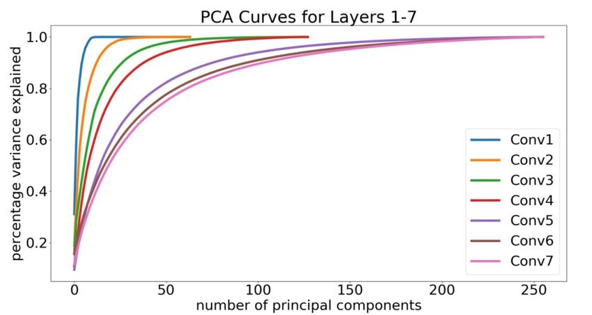
I. Garg et al.: A Low Effort Approach to Structured CNN Design Using PCA

specialized training in the form of dropout and regularization       can be adapted to suit different energy budgets. This provides
[8].                                                                 an accuracy-efficiency tradeoff knob that can be utilized for
   Practical Problems with Current Model Compression                 more error-tolerant applications where energy consumption is
Methods: The field of model compression explores ways to             a driving factor in model architecture search.
prune a network post training in order to remove redundancy.            Contributions: The main contribution of this work is
However, most of these techniques involve multiple time              a practical compression technique with explainable design
and compute intensive iterations to find an optimal threshold        heuristics for optimizing network architecture, at negligible
for compression, making it impractical to compress large             extra compute cost or time. To the best of our knowledge,
networks [6], [9], [10]. An iteration here is referred to as the     this is the first work that analyzes all layers of networks
entire procedure of training or retraining a network, instead of     simultaneously and optimizes structure in terms of both
a forward and backward pass on a mini-batch. Most standard           width and depth, without any iterative searches for thresholds
pruning techniques broadly follow the methodology outlined           for compression per layer. The additional benefits of using
in the flowchart in Fig. 1a. They start with a pre-trained           this methodology are two-fold. First, for more error tolerant
network and prune the network layer by layer, empirically            applications, where accuracy can sometimes be traded for
finding a threshold for pruning in each layer. The pruning           faster inference or lower energy consumption, this analysis
threshold modulates the fraction of pruning performed at             offers a way to gracefully tune that trade-off. Second, the
each iteration and that, in turn, affects the accuracy, which is     resultant PCA graphs (Fig. 10) are indicative of the sensitivity
estimated by retraining. This results in the two loops shown in      of layers and help identify layers that can be aggressively
the figure. Loop 1 iterates to find a suitable pruning threshold     targeted while compressing the network. This is discussed
for a layer, and Loop 2 repeats the entire process for each          in detail in section III. The effectiveness of the proposed
layer. Since these loops are multiplicative, and each iteration      methodology to optimize the structures of some widely used
involves retraining the whole network, pruning a network             network architectures is demonstrated in Section IV.
becomes many times more time and compute intensive than
training it. Some methods require only one of the two loops          II. PREVIOUS WORK ON MODEL COMPRESSION
[11], [12], but that still results in a large number of retraining   We divide model compression methods into four broad
iterations for state of the art networks. Furthermore, the           categories. The first are techniques that prune individual
resulting thresholds are not explainable, and therefore can not      weights, such as in [5], [6], [14] and [13]. These techniques
usually be justified or predicted with any degree of accuracy.       result in unstructured sparsity that is difficult to leverage in
   Proposed Method to Optimize Architecture: To address              hardware. It requires custom hardware design and limits the
these issues, we propose a low effort technique that uses            savings that can be achieved. The second category tackles
Principal Component Analysis (PCA) to analyze the network            this problem by removing entire filters. Authors of [15],
in a single pass, and gives us an optimized design in terms          [11] and [16] focus on finding good metrics to determine
of the number of filters per layer (width), and the number           the significance of a filter and other pruning criterion. Authors
of layers (depth) without the need for retraining. Here, we          of [17] pose pruning as a subset selection problem based
refer to optimality in terms of removal of redundancy. We            on the next layer’s statistic. Methods in this category that
do not claim that our method results in the most optimal             do not compromise accuracy significantly require iterative
architecture. However, it is, to the best of our knowledge, a        retraining, incurring a heavy computational and time penalty
method which optimizes a pre-trained network with the lowest         on model design. While authors of [11] analyze all layers
effort in terms of retraining iterations. The proposed method is     together, their layer-wise analysis requires many iterations.
elucidated in Fig. 1b. We start with a pre-trained network, and      Authors of [33] also remove filters by introducing multiple
analyze the activations of all layers simultaneously using PCA.      losses for each layer that select the most discriminative
We then determine the optimized network’s layer-wise width           filters, but their method iterates until a stopping condition
from the number of principal components required to explain          is reached within a layer and iterates over each layer, thus
99.9% of the cumulative explained variance. We call these the        keeping both loops active. The third category, and the one
‘significant dimensions’ of each layer and optimize the depth        that relates to our method the most, involves techniques
based on when these significant dimensions start contracting.        that find different ways to approximate weight matrices,
Once the requisite width and depth are identified, the user can      either with lower ranked ones or by quantizing such as in
create a new, randomly initialized network of the identified         [7], [10], [18], [19] and [20]. However, these methods are
width and depth and train once to get the final, efficient model.    done iteratively for each layer, preserving at least one of the
It removes both the loops since we analyze the entire network        loops in Fig. 1a, making it a bottleneck for large network
in one shot, and have a pre-defined threshold for each layer         design. Authors of [20] use a similar idea, but choose a layer-
instead of an empirical one. The proposed method optimizes           wise rank empirically, by minimizing the reconstruction error.
the architecture in one pass, and only requires a total of one       Authors of [34] group the network into binarized segments
retraining iteration for the whole network, drastically reducing     and train these segments sequentially, resulting in the second
the time required for compression. In addition, the choice of        loop, though over segments rather than layers. The binary
the threshold is predetermined and explainable, and therefore        bases of the segments are found empirically, and the method
2                                                                                                                                VOLUME 8, 2020
I. Garg et al.: A Low Effort Approach to Structured CNN Design Using PCA
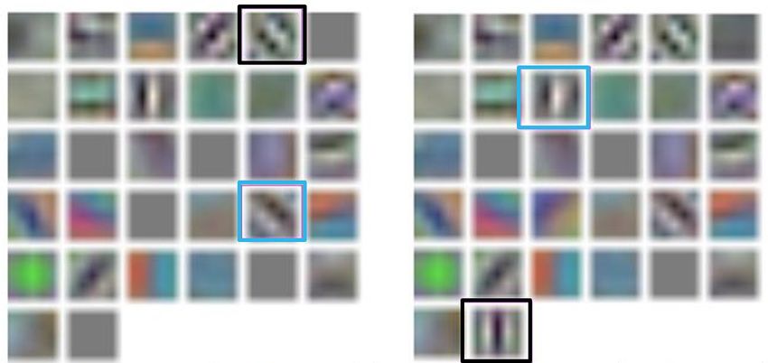
(a)
(b)
FIGURE 1: Fig. 1a shows the flowchart for standard pruning techniques. It involves two multiplicative loops, each involving
retraining of the entire network. In contrast, the proposed technique, shown in Fig. 1b only requires a single retraining iteration
for the whole network.
requires custom hardware and training methods. Authors There are other techniques that prune a little differently.
of [9] also use a similar scheme, but most of their savings Authors of [12] define an importance score at the last but one
appears to come from the regularizer rather than the post- layer and backpropagate it to all the neurons. Given a fixed
processing. The regularization procedure adds more hyper- pruning ratio, they remove the weights with scores below that.
parameters to the training procedure, thus increasing iterations While this does get a holistic view of all layers, thus removing
to optimize model design. Another difference is that we the second loop in Fig. 1a, the first loop however still remains
optimize both width and depth, and then train a new network active as the pruning ratio is found empirically. Authors of [23]
from scratch, letting the network recreate the requisite filters. learn a set of basis filters by introducing a new initialization
Aggressive quantization, all the way down to binary weights technique. However, they decide the structure before training,
such as in [21] and [22] results in accuracy degradation for and the method finds a compressed representation for that
large networks. The fourth category is one that learns the structure. The savings come from linear separability of filters
sparsity pattern during training. This includes modifying into 1x3 and 3x1 filter, but the authors do not analyze if all the
the loss function to aid sparsity such as in [30] and [29], or original filters need to be decomposed into separable filters. In
interspersing sparsifying iterations with the training iterations comparison, our work takes in a trained network, and outputs
such as in [29]. These result in extensive sparsity, but require an optimized architecture with reduced redundancy, given an
longer training or non-standard training algorithms such as accuracy target from the parent network. The work in [24]
in [27], [28], [32] and [32], and do not always guarantee shows interesting results for pruning that do not require pre-
structured sparsity that can be quickly leveraged in existing training, but they too assume a fixed level of sparsity per
hardware. A non-standard architecture is created in [31] layer. The algorithm in [35] works a little differently than
which consists of a well connected nucleus at initialization the other model compression techniques. It creates a new
and the connectivity is optimized during training. Almost smaller student model and trains it on the outputs of the
all of these works target static architectures, and optimize larger teacher model. However, there is no guarantee that
connectivity patterns rather than coming up with a new the smaller model itself is free of redundancy, and the work
efficient architecture that does not require specialized training does not suggest a method for designing the smaller network.
procedures or hardware implementations. Many of them are Along with these differences, to the best of our knowledge,
iterative over layers or iterative within a layer [25], [26]. None none of the prior works demonstrate a heuristic to optimize
of these works optimize the number of layers. depth of a network. Another element of difference is that
VOLUME 8, 2020 3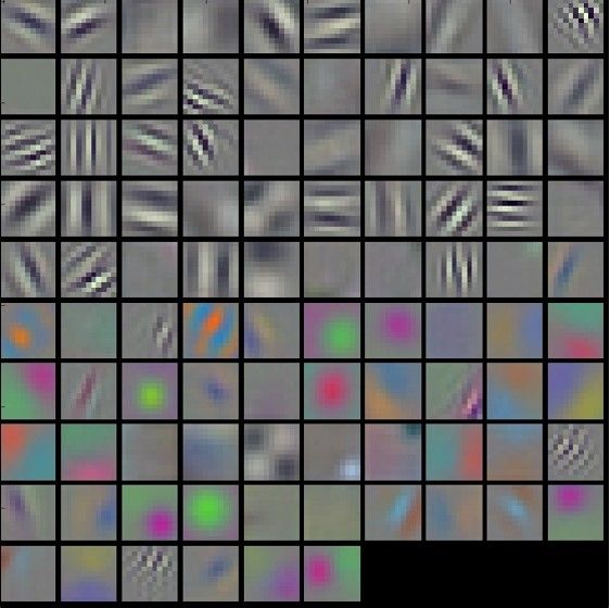
I. Garg et al.: A Low Effort Approach to Structured CNN Design Using PCA

                                                         Custom Ar-
                                              Custom
        Method Name           Loop1   Loop2              chitecture/
                                              Training
                                                         Hardware
    Deep Compression [5]       3       3         7           3
           OBD [6]             3       7         7           3
           OBS [13]            3       7         7           3
          Denton [7]           3       3         7           3
       Comp-Aware [9]          7       3         3           3
        Jaderberg [10]         3       7         3            7
        Molchanov [11]         3       3         7            7
          NISP [12]            3       7         7            7
          AxNN [14]            3       3         7           3
       Li_efficient [15]       3       3         7            7
      Auto Balanced [16]       3       3         3            7
         ThiNet [17]           3       3         7            7                        (a)                                   (b)
       SqueezeNet [18]         7       3         7           3
        MobileNet [19]         7       7         7           3         FIGURE 2: Visualization of pruning. The filter to be pruned
          Zhang [20]           3       3         7            7        is highlighted on the left and the filter it merges with is
      BinarizedNN [21]         7       7         7           3         highlighted on the right. It can be seen that the merged
        XNORNet [22]           7       7         7           3
                                                                       filter incorporates the diagonal checkerboard pattern from
         Iannou [23]           7       7         3           3
          SNIP [24]            7       7         3            7        the removed filter.
      Lottery Ticket [25]      3       7         7           3
     Imp-Estimation [26]       3       7         7            7
         NetTrim [27]          7       7         3           3
    Runtime_pruning [28]       7       3         3            7        which means that 4 sparsity percentages are tested. Methods
     Learning-comp [29]        3       7         3           3
       Learned_L0 [30]         7       7         3           3         such as [5], [7] and [11] that have both loop1 and loop2 active
      Nucleus Nets [31]        7       7         3           3         will require T*N=52 retraining iterations. Methods like [6],
    Structure-learning [32]    7       3         3            7        [26] and [29] that have only loop1 require N=4 number of
     Discrimin-aware [33]      3       3         3            7        retraining iterations and those that have only loop2 will require
     Structure-binary [34]     7       3         3           3
         Our Method            7       7         7            7        L=13 number of iterations, such as in [9], [28] and [32]. Since
                                                                       a whole retraining iteration can take many simulation days
TABLE 1: Summary of comparison of various pruning                      to converge, a large number of simulations is impractical. In
techniques. Loop 1 refers to finding empirical thresholds              contrast, our method only has 1 retraining iteration.
for pruning within a layer. Loop 2 accounts for iterations                We would also like to point out that most of the works
over layers as shown in Fig. 1a. The last two columns refer            discussed in this section are orthogonal to ours and could
to some specialized training procedures and changes to the             potentially be used in conjunction, after using our method
network architecture or a requirement of custom architecture           as a first order, lowest effort compression technique. These
respectively.                                                          differences are highlighted in tabular format in Table 1.

many of these methodologies are applied to weights, but we             III. FRAMING OPTIMAL MODEL DESIGN AS A
analyze activations, treating them as samples of the responses         DIMENSIONALITY REDUCTION PROBLEM
of weights acting on inputs. This is explained in detail in            In this section, we present our motivation to draw away
section III.                                                           from the idea of ascribing significance to individual elements
   The method we propose differs from these techniques in              towards analyzing the space described by those elements
three major ways: a) the entire network with all layers is             together. We then describe how to use PCA in the context
analyzed in a single shot, without iterations. Almost all prior        of CNNs and how to flatten the activation matrix to detect
works preserve at least one of the two loops shown in Fig.             redundancy by looking at the principal components of this
1a, while our methodology does not need either, making                 space. We then outline the method to analyze the results of
it a computationally viable way to optimize architectures              PCA and use it to optimize the network layer-wise width and
of trained networks, b) the underlying choice of threshold             depth. The complete algorithm is summarized as a pseudo-
is explainable and therefore exposes a knob to trade off               code in Algorithm 1.
accuracy and efficiency gracefully that can be utilized in
                                                                          While this is not the first work that uses PCA to analyze
energy constrained design tasks, and c) it targets both depth
                                                                       models [7], [9], the focus in this work is on a practical method
of the network and the width for all the layers simultaneously.
                                                                       of compressing pre-trained networks that does not involve
To elaborate on the number of retraining iterations needed, let
                                                                       multiple iterations of retraining. In other contexts, PCA has
L represent the number of layers and N represent the number
                                                                       also been used to initialize neural networks [36], and to
of iterations to find a suitable pruning threshold within a layer.
                                                                       analyze their adversarial robustness [37].
Networks like VGG-16 have 13 convolutional layers, and for
the sake of comparison, we assume a low estimate of N as 4,
4                                                                                                                                  VOLUME 8, 2020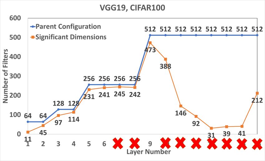
I. Garg et al.: A Low Effort Approach to Structured CNN Design Using PCA

                                                                           particular snapshot is shown and explained in Fig. 2. The
                                                                           filters before pruning are shown on the left in Fig. 2a. The
                                                                           filter that is being removed in this iteration is highlighted. The
                                                                           filters after pruning and retraining are shown on the right in
                                                                           Fig. 2b. It can be seen that the checkerboard pattern of the filter
                                                                           that was pruned out gets pronounced in the filter highlighted
                                                                           in Fig. 2b upon retraining. Before retraining, this filter looked
                                                                           similar to the filter being pruned, but the similarity gets more
                                                                           pronounced upon retraining. This pattern is repeated often
                                                                           in the animation, and leads to the hypothesis that as a filter
                                   (a)                                     is removed, it seems to be recreated in some other filter(s)
                                                                           that visually appear to be correlated to it. Since the accuracy
                                                                           did not degrade, we infer that if the network layer consists
                                                                           of correlated filters, the network can recreate the significant
                                                                           filters with any of them upon retraining.
                                                                               Given that it visually appears that each pruned out filter is
                                                                           absorbed by the one ‘closest’ to it, we tried to determine if we
                                                                           could successfully predict the retained filter that would absorb
                                                                           the pruned out filter. Pearson correlation coefficient was used
                                                                           to quantify similarity between filters. A filter was chosen to
                                                                           be pruned and it was checked if the filter that changed the
                                   (b)                                     most upon retraining the system was the one which had the
FIGURE 3: Fig. 3a: Filter to be pruned is shown in black                   maximum Pearson correlation coefficient with the filter being
and the one that got changed the most is in blue. The filter in            pruned out. The L2 distance between the filter before and after
blue also had the highest Pearson correlation coefficient [38]             retraining was used as a measure of change. Fig. 3a shows
with the filter in black. Fig. 3b: Mismatches are shown here.              an example iteration in which the filter identified as closest
The filter that is pruned out is in black, the one closest to it           to the pruned out filter, and the filter that changed the most
according to Pearson coefficient is in blue. The two filters that          upon retraining were the same. But more significantly, it was
changed the most after retraining are in pink.                             observed that there were a lot of cases where the identified
                                                                           and predicted filters did not match, as sometimes one filter
                                                                           was absorbed by multiple filters combining to give the same
A. LOOKING AT THE FILTER SPACE RATHER THAN                                 feature as the pruned out filter, although each of them had low
INDIVIDUAL FILTERS                                                         correlation coefficients individually. An illustrating example
                                                                           of such a mismatch is explained in Fig. 3b.
In an attempt to understand what happens during pruning and                    Viewing compression from the angle that each network has
retraining, an exhaustive search was carried out during every              learned some significant and non significant filters or weights
iteration for a layer in order to identify the filter that caused the      implicitly assumes that there is a static significance metric
least degradation in accuracy upon removal. This means that at             that can be ascribed to an element. This is counter-intuitive as
any iteration, all remaining filters were removed one at a time,           the element can be recreated upon retraining. Even thinking
and the net was retrained. Removal of whichever filter caused              of pruning as a subset selection problem does not account for
the least drop in accuracy was identified as the least significant         the fact that on retraining, the network can adjust its filters and
filter for that iteration. This exhaustive analysis can only be            therefore the subset from which selection occurs is not static.
carried out for small networks that do not require a long time             This motivates a shift of perspective on model compression
to train. A small 3 layer network was trained on CIFAR-                    from removal of insignificant elements (neurons, connections,
10 and visualized the effect of pruning and retraining. An                 filters) to analyzing the space described by those elements.
animation was created from the iterative results of removing               From our experiments, it would appear to be more beneficial
the identified least significant filter and retraining the model           instead to look at the behavior of the space described by
for the first layer, comprising of 32 filters. This analysis was           the filters as a whole and find its dimensionality, which is
carried out for the first layer so the filters can be effectively          discussed in the subsequent subsections.
visualized. The resulting animation can be seen at this link
[39] and gives a good insight into what occurs during pruning
and retraining. Stills from the animation are shown in Fig. 2              B. ANALYZING THE SPACE DESCRIBED BY FILTERS
and Fig. 3.                                                                USING PCA
    An interesting pattern is observed to be repeated throughout           Principal Component Analysis (PCA): Our method builds
the animation: one or more of the remaining filters appear to              upon PCA, which is a dimensionality reduction technique
‘absorb’ the characteristics of the filter that is pruned out. A           that can be used to remove redundancy between correlated
VOLUME 8, 2020                                                                                                                              5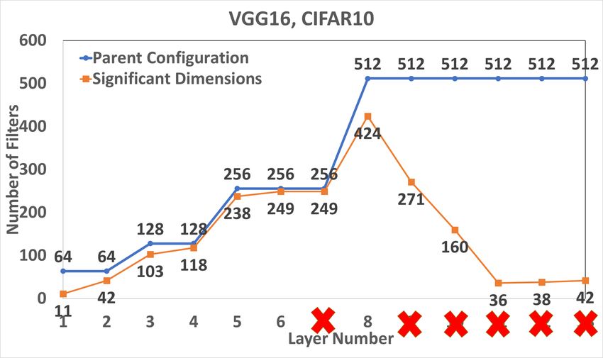
I. Garg et al.: A Low Effort Approach to Structured CNN Design Using PCA

                                                                 FIGURE 6: The output of convolving one filter with an input
                                                                 patch can be viewed as the feature value of that filter. The
FIGURE 4: Cumulative percentage of the variance of input
                                                                 green pixels in the output activation map make up one sample
explained by ranked principal components. The red line iden-
                                                                 for PCA.
tifies the significant dimensions that explain 99.9% variance.

                                                                 are highly correlated and potentially detect the same feature,
                                                                 therefore making insignificant contributions to accuracy. In
                                                                 the previous section, we deduced that pruned out filters, if
                                                                 redundant, could be recreated by a linear combination of
                                                                 retained filters without the retrained network suffering a drop
                                                                 in accuracy. This led us to view the optimal architecture
                                                                 as an intrinsic property of the space defined by the entire
                                                                 set of features, rather than of the features themselves. In
                                                                 order to remove redundancy, optimal model design is framed
                                                                 as a dimensionality reduction problem with the aim of
                                                                 identification of the number of uncorrelated ‘eigenfilters’ of
                                                                 the desired, smaller subspace of the entire hypothesis space
FIGURE 5: First layer filters of AlexNet, trained on ImageNet.   of filters in a particular layer. By using PCA, the notion of the
A considerable amount of redundancy is clearly visible in the    significance of a filter is implicitly removed, since the filters
filters.                                                         that are the output of PCA are linear combinations of all the
                                                                 original filters. It is the dimensionality which is of primary
                                                                 importance rather than the ‘eigenfilters’. We believe that
features in a dataset. It identifies new, orthogonal features    the dimensionality determines an optimal space of relevant
which are linear combinations of all the input features. These   transformations, and the network can learn the requisite filters
new features are ranked based on the amount of variance of       within that space upon training.
the input data they can explain. As an analogy, consider a           Activations as Input Data to PCA for Detecting Filter
regression problem to predict house rates with N samples         Redundancy: The activations, which are instances of filter
of houses and M features in each sample. The input to PCA        activity, are used as feature values of a filter to detect redun-
would be an NxM sized matrix, with N samples of M features       dancy between the filters generating these activations. The
among which we are trying to identify redundancy.                standard input to PCA is a 2-dimensional matrix where each
   PCA for Dimensionality Reduction: A sample output             row represents a new sample, and each column corresponds to
of PCA is shown in Fig. 4, with cumulative explained             a feature value of a particular filter for all those samples. In this
variance sketched as a function of the number of top ranked      formulation, the feature value of a filter is its output value upon
principal components. The way this graph is utilized in the      convolution with an input patch, as shown in Fig. 6. Hence a
proposed method to uncover redundancy is by drawing out          data point in the PCA matrix at the location [i,j] corresponds
the red line, which shows how many features are required for     to the activation generated when the ith input patch is acted
explaining 99.9% of the total variance in the input data. In     upon by the j th filter. The same input patch is convolved upon
this example, almost all the variance is explained by only 11    by all the filters, making up a full row of feature values for
out of 64 features. Eleven new features can be constructed as    that input patch. As many of these input patches are available
linear combinations of the original 64 filters that suffice to   as there are pixels in one output activation map of that layer.
explain virtually all the variance in the input, thus exposing   Flattening the activation map after convolution gives many
redundancy in the feature space.                                 samples for all M filters in that layer. If there are activations
   PCA in the Context of CNNs: The success of currently          that are correlated in this flattened matrix across all samples,
adopted pruning techniques can be attributed to the redun-       it implies that they are generated by redundant filters that are
dancy present in the network. Fig. 5 shows the filters of        looking at similar features in the input.
the first layer of AlexNet [40]. Many filters within the layer       Let AL be the activation matrix obtained as the output of a
6                                                                                                                            VOLUME 8, 2020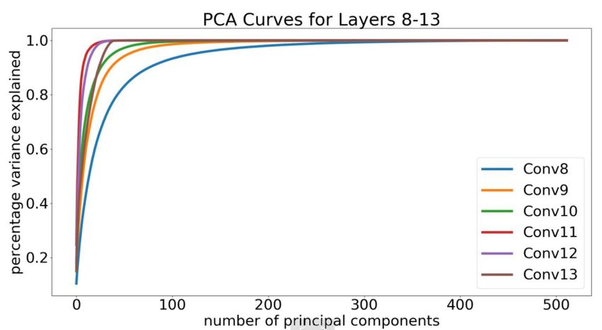
I. Garg et al.: A Low Effort Approach to Structured CNN Design Using PCA

                                                                           which we refer to as the significant dimensions for that layer,
                                                                           SL .
                                                                                                       PM̂
                                                                                                             λi
                                                                                          SL = M̂ : Pi=1 M
                                                                                                                 = 0.999
                                                                                                         i=1 λi

                                                                              These significant dimensions are used to infer the optimized
                                                                           width and depth, as explained in the subsequent sections. From
                                                                           PCA we also know the transformation that was applied to BL
                                                                           and we can apply the same transformation to the filters to
                                                                           visualize the ‘principal’ filters generated by PCA. This is
                 (a)                                  (b)                  shown in Fig. 7. Fig. 7a shows the trained filters, and Fig. 7b
                                                                           shows the ranked ‘eigenfilters’ determined by PCA. The filters
FIGURE 7: The learned filters of a convolutional layer                     are displayed according to diminishing variance contribution,
with 32 filters on CIFAR-10 are shown on the left and                      with the maximum contributing component on top left and the
the corresponding ranked filters transformed according to                  least contributing component on the bottom right.
principal components are shown on the right.
                                                                           C. OPTIMIZING WIDTH USING PCA
forward pass. L refers to the layer that generated this activation         The previous subsection outlines a way of generating PCA
map and is being analyzed for redundancy among its filters.                matrices for each layer. PCA analysis is then performed
The first filter-sized input patch convolves with the first filter         on these flattened matrices, and the cumulative variance
to give the top left pixel of the output activation map. The               explained is sketched as a function of the number of filters,
same patch convolves with all M filters to give rise to a vector           as shown in Fig. 4. The ‘significant dimensionality’ of our
∈ R1×1×M . This is viewed as one sample of M parameters,                   desired space of filters is defined as the number of uncorrelated
with each parameter corresponding to the activity of a filter.             filters that can explain 99.9% of the variance of features. This
Sliding to the next input patch provides another such sample               significant dimensionality, SL for each layer is the identified
of activity.                                                               layer-wise width of the optimized network. Since this analysis
    Suppose AL ∈ RN ×H×W ×M , where N is the mini-batch                    can be performed simultaneously for all layers, one forward
size, H and W are the height and width of the activation map,              pass gives us the significant dimensions of all layers, which is
and M is the number of filters that generated this map. Thus,              used to optimize depth as explained in the next subsection.
it is possible to collect N × H × W samples in one forward
pass, each consisting of M parameters simply by flattening                 D. OPTIMIZING DEPTH OF THE NETWORK
the matrix AL ∈ RN ×H×W ×M → BL ∈ RD×M , where                             An empirical observation that emerged out of our experiments
D = N × H × W . Since PCA is a data-intensive technique,                   was a heuristic to optimize the number of layers of the neural
we found that collecting data over enough mini batches such                network. A possible explanation for this heuristic could be
      D                                                                    arrived at by considering each layer as a transformation to
that M   is is roughly larger than 100 provides enough samples
to detect redundancy. We then perform PCA analysis on BL .                 progressively expand the input data into higher dimensions
We perform Singular Value Decomposition (SVD) on the                       until the data is somewhat linearly separable and can be
mean normalized, symmetric matrix BLT BL and analyze its                   classified with desired accuracy. This means that the width
M eigenvectors v~i and eigenvalues λi .                                    of the network per layer should be a non-decreasing function
    The trace, tr(BLT BL ) is the sum of the diagonal elements             of number of layers. However, as can be seen from the
of the sample variance-covariance matrix, and hence equal to               results in Section IV, summarized in Table 2, the number
the sum of variance of individual parameters, which we call                of significant dimensions expand up to a certain layer and
the total variance T.                                                      then start contracting. We hypothesize that the layers that
                                       M                                   have lesser significant dimensions than the preceding layer
                                       X
                       tr(BLT BL ) =          2
                                             σii =T                        are not contributing any relevant transformations of the input
                                       i=1                                 data, and can be considered redundant for the purpose of
                                                                           classification. If the significant dimensions are sketched for
The trace is also equal to the sum of eigenvalues.
                                                                           each layer, then the depth can be optimized by retaining the
                                          M
                                          X                                layers that maintain monotonicity of this graph. In Section
                         tr(BLT BL ) =          λi                         IV, we show empirical evidence that supports our hypothesis
                                          i=1
                                                                           by removing a layer and retraining the system iteratively. We
Hence, each λi can be thought of as explaining a λi /T ratio of            notice that the accuracy starts degrading only at the optimized
total variance. Since the λi ’s are ordered by largest to smallest         depth identified by our method, confirming that it is indeed a
in magnitude, we can calculate how many eigenvalues are                    good heuristic for optimizing depth that circumvents the need
cumulatively required to explain 99.9% of the total variance,              for iterative retraining.
VOLUME 8, 2020                                                                                                                            7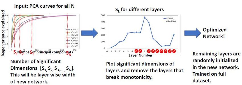
I. Garg et al.: A Low Effort Approach to Structured CNN Design Using PCA

                                                                  (a)

                                                                  (b)
FIGURE 8: Visualization of the algorithm. Fig. 8a shows how to generate the PCA matrix for a particular layer, and then find its
significant dimensions. Fig. 8b shows how to use the results of Fig. 8a run in parallel on multiple layers to deduce the structure
of the optimized network in terms of number of layers and number of filters in each layer. The structure of other layers (maxpool,
normalization etc.) is retained from the parent network.

   The methodology is summarized in the form of pseudo-                 we sketch the number of significant dimensions, and remove
code shown in Algorithm 1. The first procedure collects                 the layers that break the monotonicity of this graph. This
activations from many mini-batches and flattens it as described         decides the number of layers in the optimized network. The
in the first part of Fig. 8a. It outputs a 2 dimensional matrix         structure of the optimized network is hence obtained without
that is input to the PCA procedure in the second function. The          any training iterations. The entire process just requires one
number of components for the PCA procedure is equal to the              training iteration (line 38 in Algorithm 1), on a new network
number of filters generating that activation map. The second            initialized from scratch. This simplifies the pruning method
function, shown in the second part of Fig. 8a runs PCA on               considerably, resulting in a practical method to design efficient
the flattened matrix and sketches the cumulative explained              networks.
variance ratio as a function of number of components. It
outputs the significant dimensions for that layer as the number
                                                                        E. ADDITIONAL INSIGHTS
of filters required to cumulatively explain 99.9% of the total
variance. In the third function, this process is repeated in            Our method comes with two additional insights. First, the
parallel for all layers and a vector of significant dimensions          PCA graphs give designers a way to estimate the accuracy-
is obtained. This is shown in Fig. 8b. This corresponds to              efficiency tradeoff, and the ability to find a smaller architecture
the width of each layer of the new initialized network. Next,           that retains less than 99.9% of the variance depending on
                                                                        the constrained energy or memory budget of the application.
8                                                                                                                                   VOLUME 8, 2020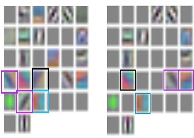
I. Garg et al.: A Low Effort Approach to Structured CNN Design Using PCA

Algorithm 1 Optimize a pre-trained model
 1:   function FLATTEN(num_batches, layer)
 2:      for batch = 1 to num_batches do
 3:          Perform a forward pass
 4:          act_layer ← activations[layer]. size: N*H*W*C
 5:          reshape act_layer into [N*H*W,C]
 6:          for sample in act_layer do
 7:              act_flatten.append(sample)
 8:          end for
 9:      end for
10:      return act_flatten
11:   end function
12:
13:   function RUN _ PCA(threshold, layer)                                 FIGURE 9: The degradation of accuracy w.r.t. target variance
14:      num_batches ← d(100 ∗ C/(H ∗ W ∗ N ))e                            to explain for different networks. Each point here is a freshly
15:      act_flatten ← FLATTEN(num_batches, layer)                         trained network whose layer-wise width was decided by the
16:      perform PCA on act_flatten, C num_components                      corresponding amount of variance to explain on the x axis.
17:      var_cumul ← cumulative sum of explained_var_ratio                 The linearity of the graphs shows that reduction in variance
18:      pca_graph ← plot var_cumul against #filters                       retained is a good estimator of accuracy degradation.
19:      SL ← #components with var_cumulS[i − 1] then
                                                                           number of significant dimensions until layer 7 and subsequent
31:               new_net.append(S[i])
                                                                           contraction from layer 8 can also be observed, leading to the
32:          else
                                                                           identification of the optimized number of layers before the
33:               break
                                                                           classifier as 7.
34:          end if
                                                                               Putting these two insights together helps designers with
35:      end for
                                                                           constrained energy budgets make informed choices of the
36:      new config: # layers ← len(new_net)
                                                                           architecture that gracefully trade off accuracy for energy. The
37:      each layer’s # filters ← SL
                                                                           final architecture depends only on the PCA graphs and the
38:      randomly initialize a new network with new config
                                                                           decided variance to retain. Therefore, given an energy budget,
39:      train new network           . Only training iteration
                                                                           it is possible to identify a reduced amount of variance to retain
40:   end function
                                                                           across all layers that meets this budget. From the PCA graphs,
                                                                           the percentage of variance retained immediately identifies
                                                                           layer-wise width, and the depth can be identified from the
Second, it offers an insight into the sensitivity of different             contraction of the layer-wise widths. For even more aggressive
layers to pruning.                                                         pruning, the graphs expose the layers most resilient to pruning
   Accuracy-Efficiency Tradeoff: Fig. 9 shows the effect of                that can be targeted further. Note that all of these insights are
decreasing the percentage of retained variance on accuracy                 available without a single retraining iteration. Thus a given
for 3 different dataset-network pairs. Each point in the graph             energy budget can directly translate to an architecture, making
is a network that is trained from scratch, whose layer-wise                efficient use of time and compute power.
architecture is defined by the choice of cumulative variance
to retain, shown on the x-axis. The linearity of this graph                IV. RESULTS FOR OPTIMIZING NETWORK
shows that PCA gives a good, reliable way to arrive at                     STRUCTURES
an architecture for reduced accuracy without having to do                  Experiments carried out on some well known architectures
empirical experiments each time. Section IV explains this                  are summarized in Table 2. Discussions on the experiments,
figure in greater detail.                                                  along with some practical guidelines for application are
VOLUME 8, 2020                                                                                                                              9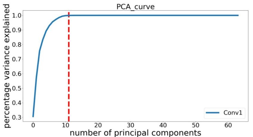
I. Garg et al.: A Low Effort Approach to Structured CNN Design Using PCA
16 and CIFAR-100/VGG-19. For both networks, a drop in
accuracy is noticed upon removing the layers where the
identified layer-wise width is still expanding. For example,
significant dimensions for CIFAR-10/VGG-16 from Table 2
can be seen to expand until layer 7, which is the number
of layers below which the accuracy starts degrading in
Fig. 11a. A similar trend is observed for CIFAR-100/VGG-
19, confirming that the expansion of dimensions is a good
criterion for deciding how deep a network should be.
C. ARCHITECTURES WITH REDUCED ACCURACY
(a) The correlation between the explained variance and accuracy
is illustrated in Fig. 9. It shows results for CIFAR-10/VGG-16
and AlexNet and VGG-19 adapted to CIFAR-100. The graph
shows how the accuracy degrades with retaining a number of
filters that explain a decreasing percentage of variance. Each
point refers to the accuracy of a new network trained from
scratch. The configuration of the network was identified by
the corresponding percentage of variance to explain, shown on
the x-axis. The relationship is approximately linear until the
unsaturated region of the PCA graphs is reached, where each
filter contributes significantly to the accuracy. The termination
point for these experiments was either when accuracy went
down to random guessing or the variance retention identified
(b)
a requirement of zero filters for some layer. For instance,
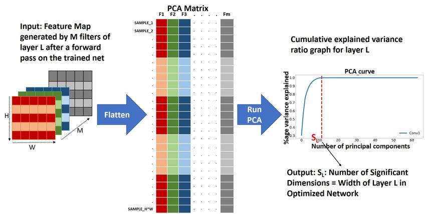
FIGURE 10: PCA graphs for different layers of CIFAR- the graph for CIFAR-100/VGG-19 stops at 80% variance
10/VGG-16_BN. Fig. 10a shows that layers 1-7 have increas- retention because going below this identified zero filters
ing sensitivity to pruning, whereas the sensitivity decreases in some layers. The linearity of this graph shows that the
from layers 8 onwards as seen in Fig. 10b. explained variance is a good knob to tune for exploring the
accuracy-energy tradeoff.
mentioned in the following subsections. PyTorch [41] was D. RESULTS AND DISCUSSION
used to train the models, and the model definitions and training Putting together the ideas discussed, the results of employ-
hyperparameters were picked up from models and training ing this method on some standard networks are summa-
methodologies available at [42]. A toolkit [43] available with rized in Table 2. Each configuration is shown as a vec-
PyTorch was used for profiling networks to estimate the tor. Each component in the vector corresponds to a layer,
number of operations and parameters for different networks. with the value equal to the number of filters in a convo-
lutional layer, and ‘M’ refers to a maxpool layer. There
A. EXPERIMENTS ON OPTIMIZING WIDTH are 5 network-dataset combinations considered, CIFAR-
Fig. 10 shows the PCA graphs of different layers for all 10/VGG-16, CIFAR-10/MobileNet, CIFAR-100/VGG-19, Im-
layers of the batch normalized VGG-16 network trained on ageNet/AlexNet and ImageNet/VGG-19. The row for signifi-
CIFAR-10. These graphs are evaluated on the activations of cant dimensions just lists out the number of filters in that layer
a layer before the action of the non linearities, flattened as that explain 99.9% of the variance. This will make up the layer-
explained in Fig. 8. It can be observed that not all components wise width of the optimized architecture. If these dimensions
are necessary to obtain 99.9% cumulative variance of the contract at a certain layer, then the final configuration has the
input. The significant dimensions are identified, that is the contracting layers removed, thus optimizing the depth of the
dimensions needed to explain 99.9% of the total variance, network. The table also shows the corresponding computa-
a new network is randomly initialized and trained from tional efficiency achieved, characterized by the reduction in
scratch with layer-wise width as identified by the significant number of parameters and operations.
dimensions. The resulting accuracy drops and savings in CIFAR-10, VGG-16_BN: The batch normalized version
number of parameters and operations can be seen from the of VGG-16 was applied to CIFAR-10. The layer-wise sig-
‘Significant Dimensions’ row of each network in Table 2. nificant dimensions are shown in Table 2. From the table,
it can be seen that in the third block of 3 layers of 256
B. EXPERIMENTS ON OPTIMIZING DEPTH filters, the conv layer right before maxpool does not add
Fig. 11 shows the degradation of retrained accuracy as the last significant dimensions, while the layer after maxpool has
remaining layer is iteratively removed, for CIFAR-10/VGG- an expanded number of significant dimensions. Hence, the
10 VOLUME 8, 2020I. Garg et al.: A Low Effort Approach to Structured CNN Design Using PCA
(a) (a)
(b) (b)
FIGURE 11: The graphs illustrate how decreasing the number FIGURE 12: The graphs show how the significant dimensions
of layers affects accuracy. Fig. 11a shows results for CIFAR- vary with layers. The layers that do not result in a monotonic
10/VGG-16 and 11b for CIFAR-100/VGG-19. For CIFAR- increase can be dropped, and are crossed out on the X axis.
100, going below 4 layers gave results highly dependent Fig. 11a shows results for CIFAR-10/VGG-16 and Fig. 11b
on initialization, so we only display results from layers 4 for CIFAR-100/VGG-19.
onwards.
means that all the filters have the same depth as the input map
conv layer before maxpool was removed while retaining the and all channels of the input map are connected to all channels
maxpool layer. In the third block, only one layer expands the of the filters, as in standard convolution without any grouping.
significant dimensions, so it was retained and all subsequent This results in increasing the number of operations and
layers were removed. The final network halved the depth to parameters by 8.5X and 8.7X respectively. The compression
7 layers with only a 0.7% drop in accuracy. The resulting algorithm is instead applied to this network, as a proxy to
significant dimensions and layer removal is visualized in Fig. the original network, and a reduction of 14.5X and 34.4X is
12a. The number of operations and parameters are reduced by seen in the number of operations and parameters respectively,
1.9X and 3.7X respectively. which translates to a reduction of 1.7X and 3.8X compared
CIFAR-10, MobileNet: The MobileNet [19] architecture to the original MobileNet architecture (with grouping). The
was trained on CIFAR-10. The configuration is shown in blocks are all reduced to just one convolutional layer, with no
Table 2. The original block configuration is shown as a 3- grouping. Even though the original network is considered to
tuple, with the first and second element corresponding to the be one of the most efficient networks, we are able to further
number of filters in the first and second convolutional layers reduce its size and computational complexity while gaining
respectively, and the third element corresponds to the stride almost a percentage point in accuracy. The number of layers
of the second convolutional layer. However, since the first reduce from 28 in the original network to 8 in the optimized
convolutional layer of each block in MobileNet has a separate network.
filter acting on each channel, we can not directly apply PCA CIFAR-100, VGG-19_BN: The analysis was expanded to
to the intermediate activation map. As a workaround, a new CIFAR-100, using the batch normalized version of VGG-19.
network with the same configuration was trained, but with the A similar trend was seen as in the previous case, and the
first convolutional layer instantiated without grouping. This optimized network consisted of 7 layers again. The resulting
VOLUME 8, 2020 11I. Garg et al.: A Low Effort Approach to Structured CNN Design Using PCA
CONFIGURATION ACCURACY #OPS #PARAMS
Dataset, Network: CIFAR-10, VGG-16_BN
Initial Config. [64, 64, ‘M’, 128, 128, ‘M’, 256, 256, 256, ‘M’, 512, 512, 512, ‘M’, 512, 512, 512] 94.07% 1X 1X
Sig. Dimensions [11, 42, ‘M’, 103, 118, ‘M’, 238, 249, 249, ‘M’, 424, 271, 160, ‘M’, 36, 38, 42] 93.76% 1.9X 3.7X
Final Config. [11, 42, ‘M’, 103, 118, ‘M’, 238, 249, ‘M’, 424, ‘M’] 93.36% 2.9X 7.7X
Dataset, Network: CIFAR-100, VGG-19_BN
Initial Config. [64, 64, ‘M’, 128, 128, ‘M’, 256, 256, 256, 256, ‘M’, 512, 512, 512, 512, ‘M’, 512, 512, 512, 512, ‘M’] 72.09% 1X 1X
Sig. Dimensions [11, 45, ‘M’, 97, 114, ‘M’, 231, 241, 245, 242, ‘M’, 473, 388, 146, 92, ‘M’, 31, 39, 42, 212, ‘M’] 71.59% 1.9X 3.7X
Final Config. [11, 45, ‘M’, 97, 114, ‘M’, 231, 245, ‘M’, 473, ‘M’] 73.03% 3.8X 9.1X
Dataset, Network: CIFAR-10, MobileNet
Initial Config:
[32, (64,64,1), (128,128,2), (128,128,1), (256,256,2), (256,256,1), (512,512,2), (512,512,1), 90.25% 1X 1X
With grouping
(512,512,1), (512,512,1), (512,512,1), (512,512,1), (1024,1024,2), (1024,1024,1)] (92.17%) (1X) (1X)
(W/o grouping)
[10, (24,21,1), (46,40,2), (103,79,1), (104,85,2), (219,167,1), (199,109,2), 1X 3.1X
Sig. Dimensions 91.33%
(235,99,1), (89,10,1), (10,2,1), (10,2,1), (10,2,1), (4,4,2), (24,16,1)] (8.5X) (28.1X)
1.7X 3.9X
Final config. [10, (24,1), (46,2), (103,1), (104,2), (219,2), (235,2)] 91.08%
(14.4X) (34.4X)
Dataset, Network: CIFAR-100, AlexNet
Initial Config. [64, 192, 384, 256, 256] 42.77% 1X 1X
Sig. Dimensions [44,119,304,251,230] 41.74% 1.6X 1.5X
Final Config. [44,119,304,251] 41.66% 2.1X 2.1X
Dataset, Network: ImageNet, VGG-19_BN
Initial Config. [64, 64, ‘M’, 128, 128, ‘M’, 256, 256, 256, 256, ‘M’, 512, 512, 512, 512, ‘M’, 512, 512, 512, 512, ‘M’] 74.24% 1X 1X
Sig. Dimensions [6, 30, ‘M’, 49, 100, ‘M’, 169, 189, 205, 210, ‘M’, 400, 455, 480, 490, ‘M’, 492, 492, 492, 492, ‘M’] 74.00% 1.7X 1.1X
TABLE 2: Summary of Results
significant dimensions and layer removal is visualized in accuracy hit. The final configuration is the same as the width-
Fig. 12b. An increase in accuracy of nearly one percent was reduced configuration shown in Table 2.
observed, presumably owing to the fact that the network
was too big for the dataset, thus having a higher chance of Limitations: One of the major limitations of this method is
overfitting. The final reduction in number of operations and that it does not apply to ResNet style networks with shortcut
parameters is 3.8X and 9.1X, respectively. connections. Removing dimensions at a certain layer that
CIFAR-100, AlexNet: To change the style of architecture connects directly to a different layer can result in recreating
to one with a smaller number of layers, the analysis was the significant dimensions in the latter layer, thus making this
carried out for CIFAR-100 dataset on the AlexNet architecture analysis incompatible. Similarly the method does not directly
and it was observed that the layer-wise depth decreased for apply to layers with grouping, since the filters do not act
all layers, but not by a large factor, as AlexNet does not seem on common inputs channels. The workaround, as discussed
to be as overparametrized a network as the VGG variants. in the case of MobileNet in section IV, is to train a new
However, the last two layers could be removed as they did not network with the same configuration but without grouping,
expand the significant dimensions, resulting in a reduction of and apply the method to that network. Another limitation is
2.1X in both the number of operations and parameters. that this method only applies to a pre-trained network. We
ImageNet, VGG-19_BN: The final test was on the Ima- do not claim that it results in the most optimal compressed
geNet dataset, and the batch normalized VGG-19 network architecture; instead, this is the lowest effort compression
was used. In the previous experiments, the VGG network that is available at negligible extra cost and can be used as
adapted to CIFAR datasets had only one fully connected layer, a first order, coarse grained compression method. More fine
but here the VGG network has 3 fully connected layers, which grained methods can then be applied on the resulting structure.
take up the bulk of the total number of parameters (86% Another point to note is that since we view the compression
of the total parameters are concentrated in the three fully method as identification of relevant subspace of filters, we do
connected layers.) Since the proposed compression technique not apply it to the fully connected layers. However, if there
only targets the convolutional layers, the total reduction in were many fully connected layers, the resulting activations
number of parameters is small. However the total number are already flattened and our method for reducing width can
of operations still reduced by 1.7X the original number with still be applied in a straightforward manner.
just a 0.24% drop in accuracy. Here, the depth did not reduce
further as the number of significant dimensions remained
non decreasing, and therefore reducing layers resulted in an
12 VOLUME 8, 2020I. Garg et al.: A Low Effort Approach to Structured CNN Design Using PCA
E. SOME PRACTICAL CONSIDERATIONS FOR THE [3] K. He, X. Zhang, S. Ren, and J. Sun, “Deep residual learning for image
EXPERIMENTS recognition,” CoRR, vol. abs/1512.03385, 2015.
[4] M. Denil, B. Shakibi, L. Dinh, M. Ranzato, and N. de Freitas, “Predicting
Three guidelines were followed throughout all experiments. parameters in deep learning,” CoRR, vol. abs/1306.0543, 2013.
First, while the percentage variance one would like to retain [5] S. Han, H. Mao, and W. J. Dally, “Deep compression: Compressing deep
neural networks with pruning, trained quantization and huffman coding,”
depends on the application and acceptable error tolerance,it arXiv preprint arXiv:1510.00149, 2015.
was empirically found that preserving 99.9% is a sweet [6] Y. LeCun, J. S. Denker, and S. A. Solla, “Optimal brain damage,” in
spot with about half to one percentage point in accuracy Advances in neural information processing systems, 1990, pp. 598–605.
[7] E. L. Denton, W. Zaremba, J. Bruna, Y. LeCun, and R. Fergus, “Exploiting
degradation and a considerable gain in computational cost. linear structure within convolutional networks for efficient evaluation,” in
Second, this analysis has only been done on activation Advances in neural information processing systems, 2014, pp. 1269–1277.
outputs for convolutional layers before the application of [8] N. Srivastava, G. Hinton, A. Krizhevsky, I. Sutskever, and R. Salakhutdi-
nov, “Dropout: A simple way to prevent neural networks from overfitting,”
non-linearities such as ReLU. Non-linearities introduce more J. Mach. Learn. Res., vol. 15, no. 1, pp. 1929–1958, jan 2014.
dimensions, but those are not a function of the number of [9] J. M. Alvarez and M. Salzmann, “Compression-aware training of deep
filters in a layer. And lastly, the number of samples to be taken networks,” CoRR, vol. abs/1711.02638, 2017.
[10] M. Jaderberg, A. Vedaldi, and A. Zisserman, “Speeding up convo-
into account for PCA are recommended to be around 2 orders lutional neural networks with low rank expansions,” arXiv preprint
of magnitudes more than the width of the layer (number of arXiv:1405.3866, 2014.
filters to detect redundancy in). Note that one image gives [11] P. Molchanov, S. Tyree, T. Karras, T. Aila, and J. Kautz, “Pruning convo-
lutional neural networks for resource efficient inference,” arXiv preprint
height times width number of samples, so a few mini-batches arXiv:1611.06440, 2016.
are usually enough to gather these many samples. It is easier [12] R. Yu, A. Li, C. Chen, J. Lai, V. I. Morariu, X. Han, M. Gao, C. Lin,
in the first few layers as the activation map is large, but in and L. S. Davis, “NISP: pruning networks using neuron importance score
propagation,” CoRR, vol. abs/1711.05908, 2017.
the later layers, activations need to be collected over many
[13] B. Hassibi, D. G. Stork, G. Wolff, and T. Watanabe, “Optimal brain
mini-batches to make sure there are enough samples to run surgeon: Extensions and performance comparisons,” in Proceedings of the
PCA analysis on. However, this is a fraction of the time and 6th International Conference on Neural Information Processing Systems,
ser. NIPS’93. San Francisco, CA, USA: Morgan Kaufmann Publishers
compute cost of running even a single test iteration (forward
Inc., 1993, pp. 263–270.
pass over the whole dataset), and negligible compared to the [14] S. Venkataramani, A. Ranjan, K. Roy, and A. Raghunathan, “Axnn:
cost of retraining. There is no hyper-parameter optimization Energy-efficient neuromorphic systems using approximate computing,”
followed in these experiments; the same values as for the in Proceedings of the 2014 International Symposium on Low Power
Electronics and Design, ser. ISLPED ’14. New York, NY, USA: ACM,
original network are used. 2014, pp. 27–32.
[15] H. Li, A. Kadav, I. Durdanovic, H. Samet, and H. P. Graf, “Pruning filters
for efficient convnets,” arXiv preprint arXiv:1608.08710, 2016.
V. CONCLUSION [16] X. Ding, G. Ding, J. Han, and S. Tang, “Auto-balanced filter pruning for
A novel method to perform a single shot analysis of any given efficient convolutional neural networks,” in AAAI, 2018.
trained network to optimize network structure in terms of both [17] J. Luo, J. Wu, and W. Lin, “Thinet: A filter level pruning method for deep
neural network compression,” CoRR, vol. abs/1707.06342, 2017.
the number of layers and the number of filters per layer is [18] F. N. Iandola, M. W. Moskewicz, K. Ashraf, S. Han, W. J. Dally, and
presented. The analysis is free of iterative retraining, which K. Keutzer, “Squeezenet: Alexnet-level accuracy with 50x fewer param-
reduces the computational and time complexity of pruning a eters andI. Garg et al.: A Low Effort Approach to Structured CNN Design Using PCA
[29] M. A. Carreira-Perpinan and Y. Idelbayev, “"learning-compression" al-
gorithms for neural net pruning,” in 2018 IEEE/CVF Conference on
Computer Vision and Pattern Recognition, June 2018, pp. 8532–8541.
[30] C. Louizos, M. Welling, and D. P. Kingma, “Learning sparse neural
networks through l_0 regularization,” arXiv preprint arXiv:1712.01312,
2017.
[31] J. Liu, M. Gong, and H. He, “Nucleus neural network for super robust
learning,” CoRR, vol. abs/1904.04036, 2019.
[32] J. Liu, M. Gong, Q. Miao, X. Wang, and H. Li, “Structure learning for deep
neural networks based on multiobjective optimization,” IEEE Transactions
on Neural Networks and Learning Systems, vol. 29, no. 6, pp. 2450–2463,
June 2018.
[33] Z. Zhuang, M. Tan, B. Zhuang, J. Liu, Y. Guo, Q. Wu, J. Huang, and
J. Zhu, “Discrimination-aware channel pruning for deep neural networks,”
in Advances in Neural Information Processing Systems, 2018, pp. 875–
886.
[34] B. Zhuang, C. Shen, M. Tan, L. Liu, and I. Reid, “Structured binary neural
networks for accurate image classification and semantic segmentation,”
in Proceedings of the IEEE Conference on Computer Vision and Pattern
Recognition, 2019, pp. 413–422.
[35] G. Hinton, O. Vinyals, and J. Dean, “Distilling the knowledge in a neural
network,” arXiv preprint arXiv:1503.02531, 2015.
[36] M. Seuret, M. Alberti, R. Ingold, and M. Liwicki, “Pca-initialized
deep neural networks applied to document image analysis,” CoRR, vol.
abs/1702.00177, 2017.
[37] P. Panda and K. Roy, “Explainable learning: Implicit generative modelling
during training for adversarial robustness,” CoRR, vol. abs/1807.02188,
2018.
[38] K. Pearson, “Note on regression and inheritance in the case of two
parents,” Proceedings of the Royal Society of London, vol. 58, pp.
240–242, 1895. [Online]. Available: http://www.jstor.org/stable/115794
[39] I. Garg, “Measure-twice-cut-once,” https://github.com/isha-garg/
Measure-Twice-Cut-Once/blob/master/exhaustive_reverse.gif, 2018.
[40] A. Krizhevsky, I. Sutskever, and G. E. Hinton, “Imagenet classification
with deep convolutional neural networks,” in Proceedings of the 25th
International Conference on Neural Information Processing Systems -
Volume 1, ser. NIPS’12. USA: Curran Associates Inc., 2012, pp. 1097–
1105.
[41] A. Paszke, S. Gross, S. Chintala, G. Chanan, E. Yang, Z. DeVito, Z. Lin,
A. Desmaison, L. Antiga, and A. Lerer, “Automatic differentiation in
pytorch,” 2017.
[42] W. Yang, “Pytorch classification,” https://github.com/bearpaw/
pytorch-classification, 2018.
[43] S. Dawood and L. Burzawa, “Pytorch toolbox,” https://github.com/e-lab/
pytorch-toolbox, 2018.
14 VOLUME 8, 2020You can also read