CNN explains tuning properties of anterior, but not middle, face-processing areas in macaque IT - bioRxiv

Page created by Mark Ayala

Current Events

English

Like
Share
Embed
Fullscreen
Slides
Download HTML
Download PDF
Abuse

←

→

Page content transcription

If your browser does not render page correctly, please read the page content below

bioRxiv preprint first posted online Jul. 3, 2019; doi: http://dx.doi.org/10.1101/686121. The copyright holder for this preprint
(which was not peer-reviewed) is the author/funder, who has granted bioRxiv a license to display the preprint in perpetuity.
It is made available under a CC-BY-NC-ND 4.0 International license.

CNN explains tuning properties of anterior, but not
middle, face-processing areas in macaque IT

Rajani Raman*, Haruo Hosoya*

Cognitive Mechanisms Laboratories, ATR International, Kyoto, Japan 619-0288

(*) corresponding authors

Abstract
A number of recent computational studies have emphasized quantitative similarity between
convolutional neural networks (CNNs) and the visual ventral stream up to the
inferotemporal (IT) cortex in the primate. However, whether such similarity holds for the
face-selective areas, a subsystem of IT, is not clear. To address this question, we extensively
investigate whether CNNs show facial tuning properties previously reported by four
experimental studies on different macaque face areas. More specifically, while simulating
the four experiments on a variety of CNN models optimized for classification, we attempted
to make a correspondence between the model layers and the macaque face areas by
quantitatively matching the tuning properties. As a result, we found that higher model
layers explained well all properties of anterior areas, while no layer simultaneously
explained multiple properties of middle areas. This observation was consistent across the
different model instances with varied architecture and dataset settings. Thus, our results
indicate that, although the near-goal representation of face-classifying CNNs has some
similarity with the primate face processing system, the intermediate computational process
might be rather different, thus calling for a more comprehensive model for better
understanding of this system.

Introduction
Recently, the neuroscience community has witnessed the rise of the deep convolution
neural network (CNN) (LeCun et al., 2015), a family of feedforward artificial neural

networks, in computational modeling of the primate visual system. CNN models trained for
behavioral goals have exhibited a remarkable similarity to ventral visual areas in terms of
stimulus-response relationship despite that the network itself was not directly optimized to
fit neural data. For example, CNN models optimized for image classification were highly
predictive of single-site and population-level neural responses in the inferotemporal (IT)
cortex (Cadieu et al., 2014; Yamins et al., 2014). In some studies, parallels along the
hierarchy have been discovered between layers of a CNN model and the intermediate
(Khaligh-Razavi and Kriegeskorte, 2014; Yamins et al., 2014; Güçlü and van Gerven, 2015) or
lower visual areas (Cadena et al., 2019); analogous parallels have been observed also in an
fMRI study (Horikawa and Kamitani, 2017). Such predictive CNN model has further been
used to generate “optimal” stimuli to validate the model (Bashivan et al., 2019). A natural
question arises here: if CNN explains overall responses in IT, then does it also explain
responses in a subsystem of IT?

Among various subsystems of IT (Downing et al., 2005; Lafer-Sousa and Conway, 2013; Sato
et al., 2013), the most well-studied is the macaque face-processing system (Tsao et al.,
2003; 2006). The subsystem forms a network consisting of multiple face-selective patches
with anatomically tight inter-connections (Moeller et al., 2008). The network putatively has
a functional hierarchy from the middle to the anterior patch areas with a progressive
increase of selectivity to facial identities and invariance in viewing angles (Freiwald and
Tsao, 2010). For each patch area, a number of tuning properties to specific facial features
have been reported in a clear and detailed manner (Freiwald et al., 2009; Freiwald and Tsao,
2010; Ohayon et al., 2012; Chang and Tsao, 2017). Given these experimental facts, the
macaque face processing system emerges as an ideal testbed to examine our question
regarding the generality of CNN as a model of higher visual processing. However, previous
studies have only touched on this direction in restricted cases involving one experiment,
one face-processing patch, or one CNN model (Chang and Tsao, 2017; Yildirim et al., 2018).

Thus, in this study, we have undertaken a more thorough investigation on whether CNN
explains previously reported tuning properties of face neurons in macaque IT (Figure 1).
More specifically, we explored a variety of CNN models that were trained for classification
with different architecture and dataset settings. We incorporated four major physiological
experiments that had been conducted on the middle lateral (ML), anterior lateral (AL), and

bioRxiv preprint first posted online Jul. 3, 2019; doi: http://dx.doi.org/10.1101/686121. The copyright holder for this preprint
(which was not peer-reviewed) is the author/funder, who has granted bioRxiv a license to display the preprint in perpetuity.
 It is made available under a CC-BY-NC-ND 4.0 International license.

 anterior medial (AM) patches: (1) view-identity tuning (Freiwald and Tsao, 2010), (2) shape-
 appearance tuning (Chang and Tsao, 2017), (3) facial geometry tuning (Freiwald et al.,
 2009), and (4) contrast polarity tuning (Ohayon et al., 2012). While simulating these
 experiments on each model, we attempted to make a correspondence between the model
 layers and the macaque face patches by matching the population-level tuning properties.
 As presented below, we discovered that higher layers tended to explain well all known
 properties of anterior patches, while no layer explained multiple properties of middle
 patches at the same time. This observation was largely consistent across the explored CNN
 models. Thus, although the near-goal representation in face processing might be similar
 between CNN and macaque, the intermediate computational process might be rather
 different, thus calling for a more comprehensive model to understand the computation in
 the primate face processing system.

 Figure 1: Schema of our investigation to compare the macaque face-processing network and
 a CNN model. We simulate previous four experiments (left image sets; top left face was
 obscured due to bioRxiv policy on the inclusion of human faces/identifiable information
 within research manuscripts) on a CNN model (bottom middle) to identify tuning properties
 (bottom right). We quantitatively compare the tuning properties between each macaque
 face patch (from the past experiment) and each CNN layer (from the present simulation) to
 find out their correspondence.

 Results
 To investigate whether CNN can explain known tuning properties of the macaque face-
 processing network, we started with a representative CNN model optimized for
 classification of face images. Our model adopted an architecture similar to AlexNet
 (Krizhevsky et al., 2012), following recent studies relating CNNs with the ventral stream

 3

(Cadieu et al., 2014; Khaligh-Razavi and Kriegeskorte, 2014; Horikawa and Kamitani, 2017).
The AlexNet architecture had seven layers in total. The first five layers were called
‘convolutional’ and performed multi-channeled local linear filters that were replicated
across the visual field. Repetition of such layers progressively increased the size of visual
receptive fields, mimicking the general structure of the visual cortex. Then, two layers
followed, which were called ‘fully connected’ and covered the entire visual field. (The
network ended with a special layer representing the class, which is ignored throughout our
analysis here.) We trained our CNN model on a large number of natural face images for
classifying facial identities (using the VGG-Face dataset; see Methods). From here on, we
refer to this network as ‘AlexNet-Face.’

For our AlexNet-Face model thus constructed, we first identified a population of face-
selective units in each layer (Methods); we call face-selective population simply
‘population’ and face-selective unit simply ‘unit’ from here on. We then proceeded to
simulation of previous four monkey experiments (Freiwald et al., 2009; Freiwald and Tsao,
2010; Ohayon et al., 2012; Chang and Tsao, 2017) on our model to see how each model
layer corresponded to each macaque face-processing patch (Figure 1).

View-Identity Tuning

In the first study that we consider (Freiwald and Tsao, 2010), it has been reported that
different macaque face patch areas (ML, AL, and AM) have different joint tuning properties
to the facial view and identity. Accordingly, we incorporated the same set of face images as
used experimentally, which consisted of 25 identities and 8 views (frontal, left and right
half-profiles, left and right profiles, up, down, and back). For each layer of our CNN model,
we first recorded the responses of all model units to those images. We then calculated the
correlation between the population responses to each pair of face images and constructed a
population response similarity matrix (RSM) of such correlations (Methods). Figure 2 shows
RSMs for layers 1, 3, 5, and 7, where the face numbers are grouped according to the view
(forming sub-matrices of size 25 × 25) and sorted by identity in the same way within each
group. (For succinctness, we present, here and hereafter, comparison results only for the
odd-numbered layers since the remaining layers generally give more or less interpolated
results of the presented layers.) In the intermediate layers (layers 3 to 5), the RSMs had
strong block-diagonal patterns, which indicated that most units had selectivity to a specific

view, similarly to ML (Freiwald and Tsao, 2010). In the top layer (layer 7), such block-
diagonal structure disappeared, but para-diagonal lines instead became prominent, which
indicated that most units had selectivity to facial identity with some degree of view
invariance, similarly to AM (Freiwald and Tsao, 2010). In addition, a mirror-symmetric
pattern in view can be seen from layers 3 to 7, somewhat similarly to AL (Freiwald and Tsao,
2010), though high correlations were observed only between the left and right profile views,
not the half-profile views. In sum, the intermediate-to-top layers gradually shifted from
view-specific to view-invariant and identity-selective, which is reasonably consistent with
the idea of functional hierarchy in the macaque face patches (Freiwald and Tsao, 2010).

Figure 2. View-identity tuning. Each plot shows the population response similarity matrix
for each layer. The pixel values of the matrix indicate the pairwise correlation coefficients
(legend) for the population responses to face images. The elements of the matrix are
grouped according to the view (indicated by the images along the axes; images were
obscured due to bioRxiv policy) with the same order of identities in each group.

The same experimental study has also reported invariance property in stimulus size
(Freiwald and Tsao, 2010). To examine such property in our model, we recorded the model
unit responses to a set of face and non-face object images of various sizes (illustrated in
Figure 3A). We then calculated, for each layer, the average response, %face
size
or %object
size
, across
the population and the stimulus set, separately for face or object images and for each image
size. We quantified the degree of invariance by size-invariance index (SII), which is defined
as the minimal fraction of image sizes at which the average population response to faces is
reasonably larger than the one to objects ( %face
size
> 1.4 %object
size
); thus, a lower SI-index
indicates a stronger size invariance (Methods). Not surprisingly, size invariance in our CNN
model strengthened along with its depth (Figure 3B). In particular, the top layer (layer 7)

bioRxiv preprint first posted online Jul. 3, 2019; doi: http://dx.doi.org/10.1101/686121. The copyright holder for this preprint
(which was not peer-reviewed) is the author/funder, who has granted bioRxiv a license to display the preprint in perpetuity.
 It is made available under a CC-BY-NC-ND 4.0 International license.

 had the strongest size invariance (SII equal to 1/4), where the average population response
 to faces (red) was always larger than the one to objects (blue) for all tested sizes. In
 comparison to the macaque, the top layer quantitatively came closest, of all layers, to the
 face patches (ML/AL/AM), which all give SII around 1/8 (Freiwald and Tsao, 2010). (The
 experimental study also investigated position invariance, but we did not incorporate this
 since position-shifted images extruded the image frame in our setting.)

 Figure 3: Size invariance. (A) Examples of face (faces were obscured due to bioRxiv policy)
 and non-face object stimuli of various sizes (the numbers beneath). (B) The average
 responses to the face images (red) and to the object images (blue) for each image size (x-
 axis) in each model layer. The ‘bline’ stands for the average baseline response to the blank
 image.

 Shape-Appearance Tuning

 In the second experimental study (Chang and Tsao, 2017), coding of facial shapes and
 appearances in the macaque face patch areas (ML and AM) has been investigated. Similarly
 to their experimental method, we constructed a face space based on the active appearance
 model (Cootes and Edwards, 2001). The face space was described by 50-dimensional
 feature vectors, consisting of 25 shape and 25 appearance dimensions, defined as follows.
 Using a set of natural frontal face images with coordinates annotated on pre-defined facial
 landmarks, the shape dimensions are the first 25 principal components (PC) of the landmark
 coordinates and the appearance dimensions are the first 25 PCs of the original face images

 6

bioRxiv preprint first posted online Jul. 3, 2019; doi: http://dx.doi.org/10.1101/686121. The copyright holder for this preprint
(which was not peer-reviewed) is the author/funder, who has granted bioRxiv a license to display the preprint in perpetuity.
 It is made available under a CC-BY-NC-ND 4.0 International license.

 that were morphed so that the landmarks matched to their mean coordinates (Methods).
 Figure 4A illustrates the first shape and first appearance dimensions by showing how varying
 these dimensions changes the image. We then randomly sampled a set of face images from
 this space and used this set for all the subsequent analyses.

 Shape-appearance preference. Following the experimental study (Chang and Tsao, 2017),
 we examined whether and how much each model unit preferred shape or appearance. For
 this, we first recorded the responses to the face images and estimated the 50-dimensional
 vector of spike-triggered average (STA), that is, the average of feature vectors of the face
 images weighted by the responses. We then computed the shape preference index (SPI),
 ( − )/( + ), where is the vector length of the shape dimensions and is the vector
 length of the appearance dimensions of the STA; a unit is considered to prefer shape when
 SPI is positive and prefer appearance when SPI is negative (Methods). Figure 4B shows the
 distribution of SPIs for each layer (blue). In the intermediate-to-higher layers (layers 5 to 7),
 most units had appearance preference, with a similar distribution to the corresponding
 experimental data on AM (pink). However, the lower layers (layers 1 to 3) broadly mixed
 both shape-preferring and appearance-preferring units, thus not particularly similar to
 either AM (pink) or ML (gray). We also examined shape-appearance preference by counting
 the number of significantly tuned units to each feature dimension; the tendency was similar
 (Figure S1A).

 Decoding performance. Following the experimental study (Chang and Tsao, 2017), we
 investigated how much information each layer contained on the face space. For this, we
 first decoded feature vectors from the population responses to each face image by linear
 regression with leave-one-out. We then measured the performance of the decoding by the
 ratio of explained variance in the actual feature values by the predicted feature values for
 each feature dimension (Figure 4C, blue). The results for the top layer (layer 7) had a good
 match with the data from AM (red). However, all lower-top-intermediate layers (layers 1 to
 5) gave results far from both AM (red) and ML (gray). In particular, no layer showed higher
 performance for shape dimensions and lower performance for appearance dimensions like
 ML (opposite to AM). We also measured the decoding performance in terms of accuracy of
 nearest-neighbor classification in the feature space; we observed a similar tendency (Figure
 S1B). Thus, in contrast to the comparison regarding the view-identity tuning experiment

 7

bioRxiv preprint first posted online Jul. 3, 2019; doi: http://dx.doi.org/10.1101/686121. The copyright holder for this preprint
(which was not peer-reviewed) is the author/funder, who has granted bioRxiv a license to display the preprint in perpetuity.
 It is made available under a CC-BY-NC-ND 4.0 International license.

 (Freiwald and Tsao, 2010), the results here reveal the lacking of ML-like properties in the
 CNN model.

 It is somewhat unintuitive, in Figure 4C, that lower layers yielded higher decoding
 performance despite the fact that they would have less face-related representations. In
 addition, we also found that, in all layers, most units showed ramp-shaped tuning curves
 along the STA and flat tuning curves along orthogonal axes to the STA (Figure S2), like in
 both ML and AM (Chang and Tsao, 2017). We continue to discuss these points in
 Discussions.

 (A)
 1st shape dimension 1st appearance dimension

 -3 0 3 -3 0 3

 (B)
 layer 1 layer 3 layer 5 layer 7
 AM ML model
 15
 # of units (%)

 10

 5

 0
 -0.5 0 0.5 -0.5 0 0.5 -0.5 0 0.5 -0.5 0 0.5
 shape preferece index

 (C)
 100
 explained variance (%)

 AM
 ML
 80 model
 60

 40

 20

 0 50 0 50 0 50 0 50
 feature dimension

 Figure 4: Shape-appearance preference. (A) Illustration of the first shape and first
 appearance dimensions for frontal faces. The images correspond to the feature vectors with
 all zero except the indicated dimension is set to -3, 0, or 3. (B) The distribution of shape-
 preference indices for each model layer (blue), in comparison to the corresponding
 distributions for ML (gray) and AM (pink) replotted from Figure 1F of the experimental study
 (Chang and Tsao, 2017). (C) Decoding performance measured by the ratio of explained
 variance in the actual feature values by the decoded feature values for each feature

 8

dimension. Each plot compares the results from a model layer (blue) with those from AM
(pink) and ML (gray), replotted from Figure 2C of the experimental study (Chang and Tsao,
2017).

View tolerance. The same experimental study also investigated view tolerance in the face
space representation in patch AM (Chang and Tsao, 2017). Accordingly, we first constructed
the feature representation for profile faces in a way compatible with frontal faces. Namely,
we built another shape-appearance face space from left profile face images, similarly to
frontal faces, and established a mapping between the frontal and profile face spaces via
linear regression; we hereafter always used feature vectors for profile faces that were
mapped to the front face space, which allowed us to use the same feature vectors for both
views of the same identity (Methods). Figure 5A illustrates the first shape and appearance
dimensions for profile faces; note the compatibility of the shown profile images with the
frontal faces in Figure 4A. For each unit, we estimated the STA from profile faces, similarly
to frontal faces, and calculated the correlation between the frontal and the profile STAs at
each feature dimension across all units in each layer (Figure 5B, red and blue). We can see
that, from lower to higher layers, the STA correlations of the first half of the appearance
dimensions (blue) increased, which indicated a gradual progression of view tolerance along
with the depth. In particular, the correlations in the top layer (layer 7) came closest, of all
layers, to the corresponding data on AM (black). Note that this result is compatible with the
view-identity tuning in the top layer shown in Figure 2. We also conducted a decoding
analysis using a mixed set of frontal and profile faces; only in the top layer, decoding
performance was similar between both views (Figure S3), consistently with AM (Chang and
Tsao, 2017).

To gain further insight, we repeated the above analysis for all available 10 non-frontal views
including right profile and half-profile views. The result for a left half-profile view (Figure
5C) shows a similar tendency to the full left profile, but the overall STA correlations were
slightly higher, indicating stronger tolerance for the half-profile view than the profile view.
This result is again consistent with Figure 2, where a closer look at the RSM of layer 7
reveals that the correlations between the half-profile and frontal views are slightly stronger
than those between the profile and frontal views. This property likely arose from our
training image set that included less images in profile views than half-profile views. Finally,

bioRxiv preprint first posted online Jul. 3, 2019; doi: http://dx.doi.org/10.1101/686121. The copyright holder for this preprint
(which was not peer-reviewed) is the author/funder, who has granted bioRxiv a license to display the preprint in perpetuity.
 It is made available under a CC-BY-NC-ND 4.0 International license.

 Figure 5D plots the mean STA correlation between the frontal and the non-frontal STAs
 (averaged over the feature dimensions) for each non-frontal view and for each layer. The
 mean STA correlation increased, thus view-tolerance became stronger, in a higher layer and
 in a view closer to the frontal view.

 (A)
 1st shape dimension 1st appearance dimension

 -3 0 3 -3 0 3

 layer 1 layer 3 layer 5 layer 7
 (B)
 AM Model
 left proﬁle
 STA correlation across units

 0.5
 0
 -0.5

 (C) left half proﬁle

 0.5
 0
 -0.5
 1 26 50 1 26 50 1 26 50 1 26 50
 feature dimension

 (D) layer: 1 3 5 7
 mean STA correlation

 0.8
 0.6

 0.4
 0.2

 view

 Figure 5: View tolerance. (A) Illustration of the first shape and first appearance dimensions
 for profile faces. The images correspond to the feature vectors with all zero except the
 indicated dimension is set to -3, 0, or 3. (B) The correlation between the frontal and the
 profile STAs across units for each dimension (x-axis; 1–25: shape, 26–50: appearance). Each
 plot compares the result from a model layer (red and blue) and AM (black) replotted from
 Figure 6D of the experimental study (Chang and Tsao, 2017). The shaded region indicates
 the 99% confidence interval of randomly shuffled data from the model. (C) Analogous result
 for the left half-profile view. (D) The mean STA correlation (averaged over the feature

 10

bioRxiv preprint first posted online Jul. 3, 2019; doi: http://dx.doi.org/10.1101/686121. The copyright holder for this preprint
(which was not peer-reviewed) is the author/funder, who has granted bioRxiv a license to display the preprint in perpetuity.
 It is made available under a CC-BY-NC-ND 4.0 International license.

 dimensions) for each non-frontal view (x-axis) against frontal view, for each layer (color; see
 legend).

 Facial Geometry Tuning

 In the third experimental study (Freiwald et al., 2009), tuning of ML neurons to local and
 global features in cartoon face stimuli has been documented. Thus, we incorporated their
 stimulus design of cartoon face images, which were parametrized by 19 different facial
 features, each ranging from −5 to +5 with ±5 corresponding to the extreme features and 0
 corresponding to the mean features (Figure 6A). We randomly generated a set of cartoon
 face images. From the responses of each unit to those cartoon face images, we estimated a
 tuning curve for each feature parameter and determined its statistical significance
 (Methods).

 Figure 6B (blue) shows how many features each unit was significantly tuned to (features-
 per-unit) in each model layer. Analogously, Figure 6C (blue) shows how many units in each
 layer were significantly tuned to each feature (units-per-feature). In both plots, the
 intermediate-to-top layers (layers 5 to 7) showed very different distributions from ML
 (gray), accommodating more units tuned to larger numbers of features and to more
 remaining features absent in ML. Curiously, the lower layers (layers 1 to 3) gave results
 somewhat closer to ML: most units were tuned to a small number of features, which were
 mostly geometrically larger features (i.e., face aspect ratio, face direction, feature assembly
 height, and inter-eye distance) rather than smaller features (related to mouth and nose). In
 addition, we observed that, in all layers, the units had tuning curves mostly ramp-shaped
 with peaks and troughs mostly at the extreme values (Figure S4), similarly to ML (Freiwald
 et al., 2009). We come back to these points in Discussions.

 11

bioRxiv preprint first posted online Jul. 3, 2019; doi: http://dx.doi.org/10.1101/686121. The copyright holder for this preprint
(which was not peer-reviewed) is the author/funder, who has granted bioRxiv a license to display the preprint in perpetuity.
 It is made available under a CC-BY-NC-ND 4.0 International license.

 (A)

 -5 -4 -3 -2 -1 0 1 2 3 4 5

 (B)
 layer 1 layer 3 layer 5 layer 7
 ML Model

 30
 # of units (%)

 20

 10

 0
 0 5 10 15 0 5 10 15 0 5 10 15 0 5 10 15
 # of features

 (C)
 face aspect ratio
 face direction
 height of assembly
 hair length
 hair thickness
 eyebrow slant
 eyebrow width
 eyebrow height
 inter-eye distance
 eye eccentricity
 eye size
 iris size
 gaze direction
 nose base
 nose altitude
 mouth-nose distance
 mouth size
 mouth top
 mouth bottom
 0 50 0 50 0 50 0 50
 # of units (%)

 Figure 6: Facial geometry tuning. (A) Examples of cartoon face images varying a feature
 parameter (inter-eye distance in this case). (B) The distribution of the number of features
 that each unit is significantly tuned to. (C) The distribution of the number of units
 significantly tuned to each feature. Each plot compares the result from a model layer (blue)
 with ML (gray) replotted from Figure 3 of the experimental study (Freiwald et al., 2009).

 Contrast Polarity Tuning

 The last experimental study (Ohayon et al., 2012) has reported that ML units had preference
 for contrast polarities between face parts in mosaic-like cartoon face stimuli (Ohayon et al.,
 2012). Thus, we again used their stimulus design of cartoon face images, which consisted of
 11 distinct face parts that were each assigned a unique intensity value varying from dark to
 light (Figure 7A). We randomly generated a set of mosaic-like cartoon faces and analyzed
 the responses of each unit to identify its contrast polarity tuning. That is, for each pair of
 face parts, A and B, out of 55 pairs in total, we determined whether the unit prefers part A

 12

bioRxiv preprint first posted online Jul. 3, 2019; doi: http://dx.doi.org/10.1101/686121. The copyright holder for this preprint
(which was not peer-reviewed) is the author/funder, who has granted bioRxiv a license to display the preprint in perpetuity.
 It is made available under a CC-BY-NC-ND 4.0 International license.

 lighter than part B (part A > part B) or the opposite (part A < part B); see Methods. As
 summarized in Figure 7B (blue), in all layers, most of the units had preferences for contrast
 polarities mainly related to the forehead, the largest geometrical area in the mosaic face.
 This result is inconsistent with the experimental finding in ML (gray), where most neurons
 were tuned to eye- or nose-related contrast polarities and the polarity directions were
 consistent across the neurons.

 (A)
 Forehead > Left Eye Forehead < Left Eye

 (B)
 model Part A > Part B
 Part A < Part B
 layer 7
 ML
 20
 0
 20

 layer 5
 20
 0
 # of units (%)

 20

 layer 3
 20
 0
 20

 layer 1
 20
 0
 20

 pair index

 Figure 7: Contrast polarity tuning. (A) Examples of mosaic-like cartoon face images with
 various intensity assignment to each face part. The first three have a larger intensity on the
 forehead than the left eye; the last three have the opposite. (B) The distribution of contrast
 polarity preferences in each model layer (blue and red) in comparison to ML (gray) replotted
 from Figure 3A of the experimental study (Ohayon et al., 2012). In each plot, the upper half
 gives the positive polarities, i.e., the units that significantly preferred part A compared to

 13

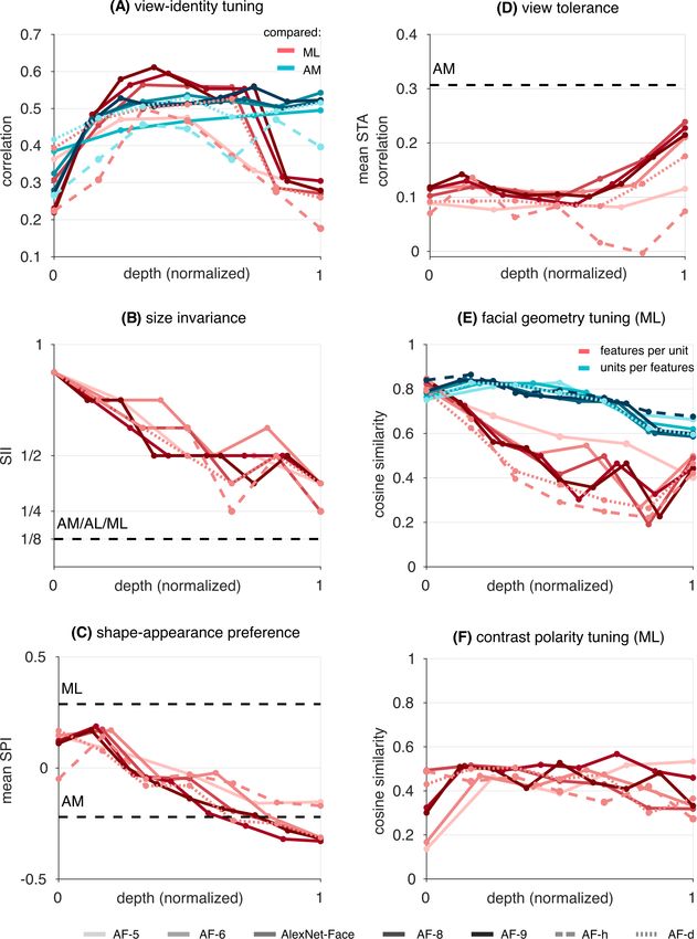
bioRxiv preprint first posted online Jul. 3, 2019; doi: http://dx.doi.org/10.1101/686121. The copyright holder for this preprint
(which was not peer-reviewed) is the author/funder, who has granted bioRxiv a license to display the preprint in perpetuity.
 It is made available under a CC-BY-NC-ND 4.0 International license.

 part B, while the lower half gives the negative polarities, i.e., the number of units that
 significantly preferred part A compared to part B. The binary table at the bottom indicate
 the 55 part-pairs; for each pair, the upper black block denotes A and the lower block denotes
 B.

 Summary of Correspondence

 To see more clearly which model layer corresponds to each macaque face patch, we next
 quantify the similarities of tuning properties; Figure 8 summarizes the results for our
 AlexNet-Face model. For each tuning property, we use a different metric to quantify
 similarity between the results from the model and the experiment. For view-identity tuning
 (Figure 8A), we use the correlation between the response similarity matrices from each
 layer (Figure 2) and each face patch (Freiwald and Tsao, 2010). For size invariance (Figure
 8B), we compare the size invariance indices obtained from each layer (Figure 3B) and each
 face patch (Freiwald and Tsao, 2010). For shape-appearance preference (Figure 8C) or view
 tolerance (Figure 8D), we compare the averages of shape-preference indices (Figure 4B) or
 mean STA-correlations (Figure 5B) from each layer and the corresponding experimental data
 (Chang and Tsao, 2017). For facial geometry tuning (Figure 8E) and contrast polarity tuning
 (Figure 8F), we use the cosine similarity between the distributions from each layer (Figure 6
 and Figure 7, respectively) and each face patch (Freiwald et al., 2009; Ohayon et al., 2012).

 Comparing between layers, AM data favor higher model layers consistently across different
 tuning properties (Figure 8A–D). However, ML data favor different layers depending on
 each tuning property: intermediate layers in view-identity tuning (Figure 8A), higher layers
 in size invariance (Figure 8B), and lower layers in other tunings (Figure 8C, E–F). Comparing
 between face patches, higher model layers also generally favor AM (Figure 8A, C). However,
 intermediate layers are somewhat inclined to ML in view-identity tuning (Figure 8A) but to
 AM in shape-appearance preference (Figure 8C). In sum, AM clearly has the best match
 with higher layers, while ML has no such clear correspondence since no layer is
 simultaneously compatible with all the investigated experimental data on ML.

 14

Model variation

How much robust are the results so far against the training condition? To address this
question, we investigated various model instances while varying the architecture and the
dataset.

First, we examined three publicly available pre-trained networks: (1) VGG-Face network
(Parkhi et al., 2015), a very deep 16-layer CNN model trained on face images, (2) AlexNet
(Krizhevsky et al., 2012), trained on general natural images, and (3) Oxford-102 network, an
AlexNet-type model trained on flower images (Methods). Figure 9 summarizes the layer-
patch comparisons for all three models (shown in different line styles), overlaid with the
plots for AlexNet-Face already given in Figure 8. Generally, the results for all four models
are similar: AM data tend to match with higher layers, while ML data do not match with any
particular layer simultaneously for all the tuning properties. It is rather surprising that
consistency can be found even in the cases of non-face training images like flowers, though
the tendency is overall weaker, in particular, view tolerance in Figure 9D. The weaker size
invariance in VGG-Face model is probably because it was trained without data
augmentation for size variation, unlike our AlexNet-Face model.

Second, to further explore the architecture space, we modified the AlexNet architecture to
construct six additional networks, where four had five, six, eight, or nine layers and two
changed the number of convolution filters in every layer to either half or double (Table S1).
We trained each model on the same face image dataset (Methods). Figure 10 summarizes
the results from these six models in addition to AlexNet-Face, where the layer numbers are
normalized. Again, the general tendency is similar across the architectures: AM corresponds
to higher layers but ML has no corresponding layer. The weak view tolerance for the model
with five layers or with half numbers of filters (Figure 10D) is probably because the depth or
the filter variety was not sufficient for gaining strong invariance.

bioRxiv preprint first posted online Jul. 3, 2019; doi: http://dx.doi.org/10.1101/686121. The copyright holder for this preprint
(which was not peer-reviewed) is the author/funder, who has granted bioRxiv a license to display the preprint in perpetuity.
 It is made available under a CC-BY-NC-ND 4.0 International license.

 (A) view-identity tuning (D) view tolerance

 compared: 0.4
 0.6 AM
 AM

 mean STA
 correlation

 correlation
 AL
 ML 0.2
 0.4

 0.2 0
 1 2 3 4 5 6 7 1 2 3 4 5 6 7
 layer layer

 (B) size invariance (E) facial geometry tuning (ML)
 features per unit
 1
 units per feature
 1

 cosine similarity
 SII

 1/2
 0.5
 1/4 AM/AL/ML
 1/8
 0
 1 2 3 4 5 6 7 1 2 3 4 5 6 7
 layer layer

 (C) shape-appearance preference (F) contrast polarity tuning (ML)

 0.5 1
 ML
 cosine similarity
 mean SPI

 0 0.5
 AM

 -0.5 0
 1 2 3 4 5 6 7 1 2 3 4 5 6 7
 layer layer

 Figure 8. Summary of comparison between layers of AlexNet-Face and face-patches. (A) The
 correlation between the response similarity matrices from each layer (Figure 2) and each
 face patch (AM/AL/ML) in Figure 4D–F of the corresponding experimental study (Freiwald
 and Tsao, 2010). (B) The size invariance index for each layer (Figure 3B) and for face patches
 (equal for AM/AL/ML) from Figure S10C of the corresponding experimental study (Freiwald
 and Tsao, 2010). (C) The mean shape-preference index for each layer (Figure 4B) with the
 mean indices for AM and ML from Figure 1F of the corresponding experimental study (Chang
 and Tsao, 2017). (D) The mean STA correlation for each layer (Figure 5B) and AM from
 Figure 6D of the corresponding experimental study (Chang and Tsao, 2017). (E) The cosine
 similarity between the distributions of the number of tuned units per feature or the number
 of tuned features per unit from each layer (Figure 6) and ML from Figure 3 of the
 corresponding experimental study (Freiwald et al., 2009). (F) The cosine similarity between
 the distributions of contrast polarity preferences from each layer (Figure 7B) and ML from
 Figure 3A of the corresponding experimental study (Ohayon et al., 2012).

 16

bioRxiv preprint first posted online Jul. 3, 2019; doi: http://dx.doi.org/10.1101/686121. The copyright holder for this preprint
(which was not peer-reviewed) is the author/funder, who has granted bioRxiv a license to display the preprint in perpetuity.
 It is made available under a CC-BY-NC-ND 4.0 International license.

 (A) view-identity tuning (D) view tolerance

 0.7 compared: 0.4
 AM
 ML AM
 0.6
 0.3

 mean STA
 correlation

 correlation
 0.5
 0.2
 0.4
 0.1
 0.3

 0.2 0
 1 2 3 4 5 6 7 1 2 3 4 5 6 7
 layer layer

 (B) size invariance (E) facial geometry tuning (ML)
 features per unit
 1 1 units per features

 0.8

 cosine similarity
 0.6
 SII

 1/2
 0.4
 1/4
 AM/AL/ML 0.2
 1/8
 0
 1 2 3 4 5 6 7 1 2 3 4 5 6 7
 layer layer

 (C) shape-appearance preference (F) contrast polarity tuning (ML)

 0.5 1
 ML
 cosine similarity
 mean SPI

 0 0.5
 AM

 -0.5 0
 1 2 3 4 5 6 7 1 2 3 4 5 6 7
 layer layer

 AlexNet-Face VGG-Face AlexNet Oxford102

 Figure 9. Summary of layer-patch comparisons for pre-trained networks in addition to
 AlexNet-Face (in different line styles; see the legend at the bottom). The format of each plot
 is analogous to Figure 8. In the view-identity tuning plot (A), we omit comparison with AL
 data for visibility. In the size invariance plot (B), we slightly shift each curve vertically for
 visibility. Since VGG-Face model was too large to fully analyze, we show results from five
 chosen intermediate-to-top layers.

 17

bioRxiv preprint first posted online Jul. 3, 2019; doi: http://dx.doi.org/10.1101/686121. The copyright holder for this preprint
(which was not peer-reviewed) is the author/funder, who has granted bioRxiv a license to display the preprint in perpetuity.
 It is made available under a CC-BY-NC-ND 4.0 International license.

 Figure 10. Summary of layer-patch comparisons for different architectures changing the
 depth or the number of convolution filters, indicated by different colors or line styles; AF-5 to
 9 varied the depth; AF-h halved and AF-d doubled the number of filters in each layer; see the
 legend at the bottom. The format of each plot is similar to Figure 8, except that x-axis shows
 the normalized depth (0 corresponds to the lowest layer and 1 to the highest layer).

 18

Discussions
In this study, we have investigated whether CNN can serve as a model of the macaque face-
processing network. While simulating four previous physiological experiments (Freiwald et
al., 2009; Freiwald and Tsao, 2010; Ohayon et al., 2012; Chang and Tsao, 2017) on a variety
of CNNs trained for classification, we examined whether the results quantitatively match
between each model layer and each face patch. We found that higher model layers tended
to explain well properties of the anterior patch, while none of the layers simultaneously
captured those of the middle patch. This observation was largely consistent across the
different model instances. Thus, despite the prevailing view linking CNNs and IT, our results
indicate that the intermediate computational process in the macaque face processing
system might be rather different from CNN and therefore requires a more refined model to
clarify the underlying computational principle.

Some previous studies have addressed a similar question but in a smaller scale. In one
study (Yildirim et al., 2018), the authors tested view-identity tuning on a CNN model in
comparison to physiology (Freiwald and Tsao, 2010) and gave a similar result to ours (Figure
2). However, they considered no other physiological experiment. In another study (Chang
and Tsao, 2017), the authors trained a smallish face-classifying CNN model and tested
shape-appearance tuning. They showed that the top layer exhibited appearance preference
and ramp-flat tuning consistent with their experimental result on AM (Chang and Tsao,
2017) and with our results (Figure 4B and Figure S2, layer 7). However, they did not
consider any other part of the same experiment (decoding performance and view tolerance)
or any other layer than the top, or any comparison with ML, not to say about different
experiments or model instances. Thus, the comparisons undertaken in our study here are
far more thorough and extensive than those previous studies.

What insight did we gain from our results? First, later stages in both CNNs and the macaque
face-processing system have similarity in terms of strong invariance properties in size and
view (Figure 2, Figure 3B, and Figure 5B). Although invariance properties in CNN are
generally well-known, such fine-grained similarity to physiology in the view-tolerant
appearance code would be somewhat beyond expectation (Figure 5B). Second, later stages
in both systems are also similar in terms of dominant appearance representation (Figure 4).

However, shape representation, in contrast, is dominant in intermediate stages in macaque
but conspicuously lacking in intermediate-to-higher stages in CNN (Figure 4 and Figure 6).
This may be because shapes turn out to be relatively unimportant features for classification
and thus neglected during the model training (Baker et al., 2018). This implies that the goal
of the face-processing system may not be merely classification. On the other hand, we have
found several somewhat unintuitive results in lower layers: (1) facial shape tuning (Figure 4B
and Figure 6), (2) higher decoding performance than higher layers (Figure 4C), and (3) ramp-
shape tuning along STA axis and flat tuning along the orthogonal axis (Figure S2 and Figure
S4). We speculate that these are partly because lower-layer units, although simple,
localized feature detectors (e.g., Gabor filters), can in fact easily interact with stimulus
parameters controlling shape feature dimensions or local facial geometry. In addition,
lower layers have much weaker nonlinearity so that linear decoding would become easier.
Nonetheless, we consider that such low-level units should not be qualified as face-selective
from the first place, but might have been misjudged so by the standard criterion due to the
specific image statistics of face images (e.g., emphasis on eyes); future studies might
therefore need to consider revision of the criterion itself.

In general, relationship between artificial and biological neural networks has been a
recurring question. Since the brain has a number of sub-networks with a hierarchical
structure, it is tempting to hypothesize that such sub-network is optimized for some
behavioral goal. Indeed, in a classical study (Zipser and Andersen, 1988), it has been shown
that a neural network trained for a coordinate transformation task exhibits, in the
intermediate layer, properties related to spatial location similar to primate parietal area 7a.
More recently, as already discussed in the introduction, numerous studies have argued that
CNNs trained for image classification have layers similar to higher (Cadieu et al., 2014;
Khaligh-Razavi and Kriegeskorte, 2014; Yamins et al., 2014; Horikawa and Kamitani, 2017),
intermediate (Khaligh-Razavi and Kriegeskorte, 2014; Yamins et al., 2014; Güçlü and van
Gerven, 2015), or lower (Cadena et al., 2019) areas in the monkey or human visual ventral
stream. Analogously, some studies have discovered layer-wise correspondence between
CNNs trained for audio classification and the human auditory cortex (Kell et al., 2018) or the
monkey peripheral auditory network (Koumura et al., 2019). Note that all these studies
have offered positive answers to the correspondence question, which stresses the

generality of explanatory capabilities of goal-optimized neural networks. However, the
same story might not go all the way through. For the macaque face-processing network,
our study here could not find a CNN layer corresponding to the intermediate stage (ML). In
addition, some recent studies have pointed out potential representational discrepancies
between CNN and the ventral stream from behavioral consideration (Baker et al., 2018;
Groen et al., 2018; O’Toole et al., 2018; Rajalingham et al., 2018). (See also the related
discussion on the ‘computational gap’ below.)

One should note that there are, in general, two fundamentally different approaches for
comparing a model with the neural system. In one approach, which is more traditional and
taken in our study here, a given model is tested whether it exhibits tuning properties
compatible with prior experimental observations (‘tuning approach’). In the other
approach, which is recently more popular (Cadieu et al., 2014; Yamins et al., 2014; Kell et al.,
2018), a given model is used as a basis function and a linear regression fitting is conducted
from model responses to actual neural responses for predicting new neural responses
(‘prediction approach’). In the tuning approach, although the comparison is arguably more
direct in the sense of involving no fitting, tuning experiments have often been criticized for
biased and subjective stimulus design and for use of degenerate summary statistics.
Therefore showing consistency with experimentally observed tuning may not be sufficiently
supportive evidence for the model. Note that, nevertheless, showing clear inconsistency is
strongly falsifying evidence, from the logical contraposition of ‘if the model behaves
similarly to the neural system, then it should reproduce the tuning.’ Our comparison with
ML is one such example. In the prediction approach, on the other hand, since a model can
be tested with an arbitrary (randomly selected) set of stimulus, the aforementioned
criticism would not occur. However, because of the necessity of linear fitting, the
comparison becomes somewhat more indirect: the correspondence is made between an
actual neuron and a ‘synthetic neuron,’ i.e., the output of a linear model after fitting (Cadieu
et al., 2014; Khaligh-Razavi and Kriegeskorte, 2014; Yamins et al., 2014; Eickenberg et al.,
2017). Indeed, one example of computational gap between CNN and IT neural responses
has been raised in Fig. 7 of the study by Cadieu et al. (Cadieu et al., 2014), where the
population similarity matrices from IT and the CNN top layer were strikingly different
without fitting, although very similar with fitting; one might therefore argue that it is a CNN

plus a linear regression, not a CNN itself, that has predicted neural responses. However,
neither of the two approaches, tuning or prediction, seems to be better than the other.
Rather, both are looking at different aspects of the visual representations and therefore
should probably continue to be used for further deepening our understanding.

If CNN does not fully explain all the facial tuning properties, then what are other possible
models? Some hints can be found in prior theoretical studies. First, unsupervised learning
can give rise to feature representations from the statistics of input images. Although such
theory has more traditionally been used for early vision (Olshausen and Field, 1996;
Hyvärinen and Hoyer, 2001; Schwartz and Simoncelli, 2001; Hosoya and Hyvärinen, 2015),
recent studies have reported its possible contributions in facial tuning properties. For
example, sparse coding of facial images can produce facial-part-like feature representations
and explain the facial geometry tuning in ML (Hosoya and Hyvärinen, 2017); PCA-based
learning can produce global facial feature representations and explain mirror-symmetric
tuning like in AL (Leibo et al., 2017). Second, feedback processing is ubiquitous in the visual
system and therefore likely important, but crucially missing in CNN. One standard
theoretical approach to incorporating feedbacks is to use a generative model. Such theory
has also been typical for modeling early vision (Olshausen and Field, 1997; Rao and Ballard,
1999; Hosoya, 2012), some recent studies have raised potential importance in higher vision.
For example, a particular generative model, called mixture of sparse coding models, has
been employed to represent an organization of multiple modules of model units with
competitive interaction (Hosoya and Hyvärinen, 2017), which has endowed the units with a
global face detection capability similar to the neural face selectivity. In a completely
different approach, an inverse-graphics-based generative model has been investigated,
where a feedforward network employed to infer facial parameters has exhibited view-
identity tuning properties similar to ML, AL, and AM in different layers (Yildirim et al., 2018).
Third, although invariance properties can emerge from supervised learning as in CNN, other
approaches exist. Some theories have used spatial image statistics to explain position or
phase invariance in early vision (Hyvärinen and Hoyer, 2001; Karklin and Lewicki, 2008;
Hosoya and Hyvärinen, 2016). However, for explaining more complex invariance properties
in higher vision, the temporal coherence principle (Földiák, 1991), which learns the most
slowly changing features, has been more commonly used (Einhäuser et al., 2005; Farzmahdi

et al., 2016; Leibo et al., 2017) and experimentally tested (Cox et al., 2005). Lastly, although
combining invariance learning into a generative model is theoretically not so obvious, one
recent development has achieved it (Hosoya, 2019). In sum, for clarifying the
computational principle underlying the primate face-processing system, it seems crucial to
view this system as not merely a classifier but having a richer repertoire of visual processing.
We hope that investigation in this direction, together with the results in the present work,
will eventually guide us to better understanding of general visual object processing.

Methods

Convolutional Neural Network (CNN)

CNN is a family of feedforward, multi-layered computational models (LeCun et al., 1998),
which has originally been inspired by the mammalian visual system. CNN allows for a
variety of architecture design, stacking an arbitrary number of layers with different
structural parameters. Each layer in CNN undergoes several operations. The layer typically
starts with convolutional filtering, which applies an identical multi-channel linear filter to
every local subregion throughout the visual field. Then, the results are given to a nonlinear
function, ReLU( ) = max(0, ), at each dimension, for ensuring non-negative outputs. The
layer is optionally preceded by pooling and normalization. Pooling gathers the incoming
inputs within a local spatial region by taking the maximum. Normalization normalizes the
outputs by dividing the incoming inputs by their squared norm. Generally, a CNN
architecture consists of multiple such layers, by which it progressively increases the
effective receptive field sizes and eventually achieves a non-linear transform of the input
from the whole image space to a space of interest (i.e., class). Often, the last several layers
of a CNN architecture have convolutional filters covering the entire visual field, thus called
fully-connected layers.

Each layer operation is closely related to some neural computation discovered in
neurophysiology. Convolutional filtering mimics V1 simple cells, which replicate their
receptive field structures across the visual field (Hubel and Wiesel, 1962). The nonlinear
function proxies for neural thresholding giving rise to non-negative values of firing rates.
Pooling comes from the classical notion that V1 complex cells gather the outputs from V1

simple cells to achieve position or phase invariance (Hubel and Wiesel, 1962; Alonso and
Martinez, 1998). Normalization stems from a gain-controlling phenomenon that is widely
observed in the cortex and often explained by the well-known divisive normalization theory
(Heeger, 1992). Further, the repetition of layers of similar processes is inspired by the
hierarchy of the visual cortex, for which the gradual increase of receptive field sizes and the
congruent micro-circuit structures are well known (Felleman and Van Essen, 1991). To dive
deep in CNN, see introductory materials (Goodfellow et al., 2016; Rawat and Wang, 2017).

Trained CNN Models

We show, most in detail, the results from a representative CNN model called ‘AlexNet-Face.’
This CNN model has the same architecture as AlexNet (Krizhevsky et al., 2012) with five
convolutional layers followed by two fully connected layers. (The network ends with a
special layer for representing classes, but we ignore it in our analysis.) The architecture
parameters are given in Table S1. We trained it for the classification task using the VGG-
Face dataset (Parkhi et al., 2015), which contains millions of face images of 2622 identities.
We augmented the dataset with size variation, allowing four-times downsizing. We
performed the training by minimizing the cross-entropy loss function, a commonly used
probabilistic approach to measure the error between the computed and given outputs
(Goodfellow et al., 2016); we used the stochastic gradient descent method with momentum
(SGDM) as optimizer. The resulting CNN model gave classification accuracy 72.78% for held-
out test data. (This score is somewhat lower than state-of-art face recognizing deep nets,
which typically go over 90% of accuracy. This is likely because our size-varied data
augmentation yielded very small images that would be difficult to classify, e.g., Figure 3A).

To test robustness of our results against structural change to the model, we incorporated a
set of six additional model instances modifying the architecture of AlexNet. Four of them
changed the number of layers to five, six, eight, and nine. We designed the specific
architectures for these by changing only the convolutional layers, keeping the overall
structure of increasing receptive field sizes. The remaining two models changed the number
of filters in every layer, one halved and one doubled. The architecture parameters of the
additional models as well as their classification accuracies are given in Table S1.

For all implementation, we used Matlab with Deep Learning
Toolbox (https://www.mathworks.com/products/deep-learning.html) as well as Gramm
plotting tool (Morel, 2018) for visualization.

Pre-trained CNN Models

To further test robustness, we included three publicly available pre-trained CNN models
using very different architecture or dataset, namely, VGG-Face network (Parkhi et al., 2015),
AlexNet (Krizhevsky et al., 2012), and Oxford-102 network. The VGG-Face network is a very
deep 16-layer CNN model that has been trained on VGG-Face database for face
classification (with no data augmentation for size variation). AlexNet is the original network
trained on ImageNet database (Deng et al., 2010) for natural image classification.
Oxford102 is an AlexNet network that has been ‘fine-tuned' for the classification of flower
images in Oxford-102 dataset (Nilsback and Zisserman, 2008). We imported these three
network models from a public repository (https://github.com/BVLC/caffe/wiki/Model-Zoo).

Experiments

On each CNN model, we first identified face-selective units and then proceeded to
simulation of four macaque experiments on these face-selective units. The specific
procedures are summarized as follows.

Face-Selective Population Estimation

We determined the face-selectivity of a unit by following the general approach used in
experiments on IT (Freiwald et al., 2009; Freiwald and Tsao, 2010). That is, we first recorded
the responses of the unit to a set of 50 natural frontal faces from the FEI image database
(http://fei.edu.br/~cet/facedatabase.html) and to a set of 50 non-face object images
obtained from the Web. Then, from the average responses to the faces, face , and non-face
object images, object , above the baseline response to the blank image (all zero pixel-values),

we estimated the Face Selective Index, FSI = J face − object L/J face + object L. FSI was

set to 1 when face > 0 and object < 0, and to -1 when face < 0 and object > 0. We
N
judged a unit as face-selective if FSI > O, that is, the unit responded to face images, on

average, twice as strongly as to non-face object images. (Zero FSI, for instance, implies an
equal average response to face and non-face images.) For the simulation of shape-

You can also read