SAR image wave spectra to retrieve the thickness of grease pancake sea ice using viscous wave propagation models - Nature
←
→
Page content transcription
If your browser does not render page correctly, please read the page content below
www.nature.com/scientificreports
OPEN SAR image wave spectra to retrieve
the thickness of grease‑pancake
sea ice using viscous wave
propagation models
1*
Giacomo De Carolis , Piero Olla2,3 & Francesca De Santi 1
Young sea ice composed of grease and pancake ice (GPI), as well as thin floes, considered to be the
most common form of sea ice fringing Antarctica, is now becoming the “new normal” also in the
Arctic. A study of the rheological properties of GPI is carried out by comparing the predictions of
two viscous wave propagation models: the Keller model and the close-packing (CP) model, with
the observed wave attenuation obtained by SAR image techniques. In order to fit observations, it
is shown that describing GPI as a viscous medium requires the adoption of an ice viscosity which
increases with the ice thickness. The consequences regarding the possibility of ice thickness retrieval
from remote sensing data of wave attenuation are discussed. We provide examples of GPI thickness
retrievals from a Sentinel-1 C band SAR image taken in the Beaufort Sea on 1 November 2015, and
three CosmoSkyMed X band SAR images taken in the Weddell Sea on March 2019. The estimated GPI
thicknesses are consistent with concurrent SMOS measurements and available local samplings.
Climate change has led in the last decade to a dramatic reduction in the extent and the thickness of sea ice in
the Arctic region during the summer season. As a result, the marginal ice zone (MIZ), which is the dynamic
transition region separating the ice pack from the open ocean, has become increasingly exposed to the wind and
the wave a ctions1,2. In these conditions, water freezes to form a thin slurry of frazil ice, called grease ice, with
thicknesses up to 10–30 cm depending on the windy c onditions3–5. As the freezing process continues, it leads to
a further stage of development of the grease ice layer, which consolidates into pancake-shaped ice bodies, called
pancake ice6,7. Grease and pancakes ice (GPI) have always been relatively ubiquitous in the Antarctic MIZ8, and
extensive GPI formation has recently been observed also in the western Arctic, as documented during the field
campaign in fall 20159.
Investigations to determine how an increase in GPI may affect the climate, possibly leading to local warming
in the far north, are ongoing. These studies and their implementation in climate models clearly require some
tools to monitor the GPI’s properties, especially as regards its thickness.
As the extent of GPI fields is controlled by the presence of waves that usually come from the open ocean,
the relationship between wave attenuation rates and GPI rheology is a key factor to understand and model the
evolution of the ice cover. Given the large scale separation between pancakes and the typical wavelength, a good
approximation to describe the interaction with ocean waves is to represent GPI as a continuum10,11. Validation
and calibration of any GPI wave model are tasks that cannot be entrusted to in situ activities, due to the vast extent
of the GPI fields, their intrinsic dynamic nature, and the harsh environment where they develop. A systematic
and extensive characterization of the spatio–temporal distribution of GPI can however be carried out through
remote sensing by exploiting the capability of SAR imaging techniques to measure the full ocean wave directional
spectrum12. By tracking the SAR observed ocean wave spectrum (or its peak, as done in pioneer studies such
as13), from open sea throughout the GPI cover, it is indeed possible to measure wave dispersion and attenuation.
A dedicated GPI wave model can then be used to relate the modifications in the wave propagation with GPI
properties such as its thickness and mechanical properties.
The literature on the application of SAR spectral inversion techniques to GPI thickness retrieval dates back
apers14–17, the GPI thickness was estimated by a adopting a mass-loading scheme, in
at least to 1997. In earlier p
1
National Research Council of Italy (CNR), Institute for Electromagnetic Sensing of the Environment (IREA),
Milan 20133, Italy. 2National Research Council of Italy (CNR), Institute of Atmospheric Science and Climate
(ISAC), Cagliari 09042, Italy. 3National Institute for Nuclear Physics (INFN), Cagliari 09042, Italy. *email:
giacomo.decarolis@cnr.it
Scientific Reports | (2021) 11:2733 | https://doi.org/10.1038/s41598-021-82228-x 1
Vol.:(0123456789)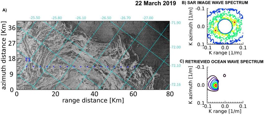
www.nature.com/scientificreports/
which GPI is represented as a continuum of non-interacting point-like mass loads on the sea surface10. How-
ever, the success of the approach was limited by the excessively high values of the thickness resulting from SAR
inversion.
Later papers18–20 abandoned the mass-loading approach for the more realistic representation of GPI proposed
by Keller11. The Keller’s model pictures the GPI layer as a viscous fluid of given thickness h and effective viscosity
ν floating over an infinitely deep, inviscid water column. The GPI effective viscosity is an unknown parameter,
with experimental evidence suggesting strong variability with respect to the composition of the sea ice matrix. As
an example, wave buoy attenuation data collected in the Weddell Sea over GPI fields with pancakes thicknesses
up to 50 cm, compared with the Keller’s models, revealed a variability of GPI effective viscosity values spanning
the range 10−1 − 103 m2 /s21, without a clear relationship with the GPI layer thickness.
Other viscous layer models have been proposed to describe wave propagation in ice/water systems. We can
mention the two-layer viscous model (TLV), which assumes the water underneath the ice cover to have a finite
viscosity, possibly due to turbulent e ffects22, and the viscoelastic model, which treats the ice layer as a viscoelas-
tic medium23. All these generalizations of the Keller’s model, however, seem unable to significantly reduce the
variability of the effective ice v iscosity24,25.
We argue that at least part of the variability of the effective viscosity required by the Keller’s model to describe
the properties of GPI, may stem from attempting to treat the ice layer as a homogeneous medium. The close-
packing (CP) m odel26 makes a first attempt to explicitly take into account the inhomogeneity of GPI, by assum-
ing that pancakes are confined to a fictitious layer of infinitesimal thickness, lying on top of the grease ice layer
and modifying the wave stress at the upper surface. The CP model was tested on field data from the Arctic and
the Antarctic, along with Keller’s and TLV m odels25. Fitting of the field data was possible with all the models
considered, but only the CP model produced GPI effective viscosities in a range consistent with that of grease
ice in laboratory experiments (≈ 2.5−3 × 10⁻² m2 /s)27.
The SAR inversion procedure consists of the following four steps:
• Estimation of the directional open ocean wave spectrum S̃w (k) at the boundary of the ice-field from the avail-
able SAR image, using the closed form expression of the non-linear ocean-to-SAR spectral form described
in Hasselmann and Hasselmann (1991)12 and later modified for the SAR image cross-spectral t ransform28.
• Simulation of the ocean wave spectrum in sea ice Si (x, k; h, ν). It is assumed that GPI cover alters the incom-
ing ocean wave spectrum according to the following expression19,29:
Si (x, k; h, ν) = S̃w (k) exp[−2q(h, ν)�(ek , x)], (1)
where �(ek , x) is the distance traveled from the ice edge to the position x by the wave of wavenumber k
heading the direction ek and q(h, ν) is the wave damping predicted by the viscous wave propagation model
considered.
• Transformation of the simulated wave spectrum to a SAR image spectrum Pi (τ ; h, ν; x, k)), as described i n12,
• Comparison of the modeled and the observed SAR spectrum, P̃i (τ ; x, k), through the following cost function
min �(τ , x; h, ν) = [R(P̃i (τ ; x, k) − Pi (τ ; h, ν; x, k))]2 d2 k, (2)
ν,h
where R stands for the real part of the argument and τ the temporal separation between the SAR looks (in
the cases in exam τ = 0).
The procedure is therefore characterized by the choice of the viscous wave propagation model to predict the
wave damping. Predictions on q(h, ν) provided by the TLV and the viscoelastic models have been carried out
elsewhere and showed not to differ significantly from the ones by the Keller’s model at a given GPI’s thickness
and viscosity24,25. The present study is therefore limited to the Keller’s and the CP model. An outline of the models
is presented in the “Methods” section.
In the former SAR inversion schemes, the couple (h, ν) minimizing the distance—parameterized by the cost
function—between simulated and observed SAR image spectrum, was then assigned to the GPI portion trave-
led by the waves. However, we have observed that the intrinsic structure of GPI viscous wave models does not
allow one to identify an absolute minimum of the cost function. Instead, deep valleys in the parameters’ space
can be observed, which leads to important consequences on the procedure of ice thickness r etrieval25. The valleys
follow power-law curves ν ∝ hα, where α is characteristic of the specific GPI wave model considered, and result
in an underdetermined minimization problem. In order to infer a unique minimizing couple (h, ν ), a relation-
ship between effective ice viscosity and thickness has to be empirically formulated through a calibration process.
We perform such calibration thanks to a study conducted in the Odden Ice Tongue, Greenland Sea. The
Odden Ice Tongue developed in 1996/1997 and was characterized by massive presence of GPI. The process was
extensively documented by SAR imagery, and GPI thickness maps obtained from a specifically developed model
were available30. Both in the case of the Keller’s and the CP model, calibration produces an effective viscosity
which is a monotonically increasing function of the ice thickness.
The proposed calibration technique is eventually tested on four different SAR images gathered by Sentinel-1A
and COSMO-SkyMed, representing case studies for the Arctic and for the Antarctic MIZ, respectively. The SAR
retrieved GPI thicknesses result in good agreement with the concurrent SMOS measurements and the available
local samplings.
Scientific Reports | (2021) 11:2733 | https://doi.org/10.1038/s41598-021-82228-x 2
Vol:.(1234567890)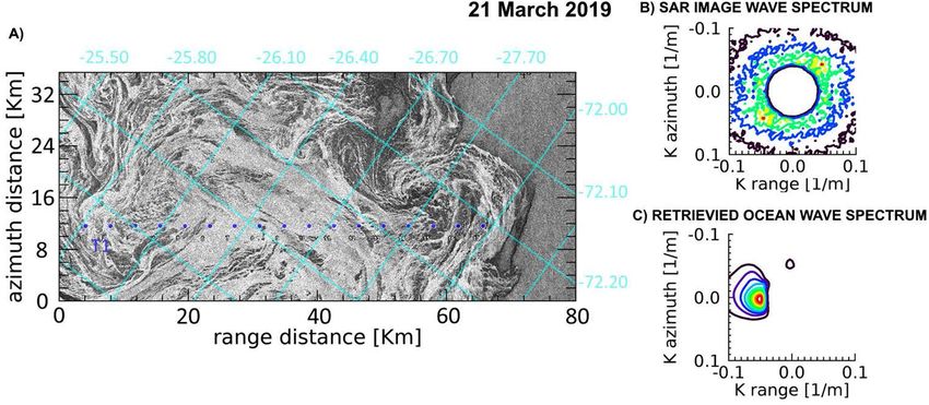
www.nature.com/scientificreports/
Results
Empirical constitutive equation for GPI viscosity. The analysis of a set of wave buoy data gathered in
the advancing MIZ of the Weddell Sea covered by GPI clearly revealed that the GPI wave attenuation rates scale
with the “equivalent solid ice thickness”21
h = Cgr hgr + Cp hp , (3)
where C and h are respectively the concentration and thickness of grease (gr) and pancake (p) ice. The relation
is physically sound, as it states a proportionality between wave decay and ice volume per unit area of the region
of the sea traveled by the waves. We point out that the effective ice thickness is the quantity most relevant to the
overall changes in ice volume, and is used in numerical dynamic-thermodynamic sea ice m odels31. Hereafter we
will refer to the GPI thickness as the effective ice thickness of the GPI layer.
As discussed in the “Methods” section (see Eqs. (21), (22) and (25)), minimization of the cost function
does not fix uniquely the parameters h and ν in the given SAR image; instead, a power law expression is obtained:
ν = βhα , (4)
where α is specific of the GPI model utilized:
αCP = 3, αK = −1, (5)
respectively, for the CP and the Keller’s model25. On the contrary, the parameter β appears to be strongly depend-
ent on the specific SAR image portion examined, and therefore on the physical properties of the sea ice layer and
of the wave spectrum in it. Since the cost function in Eq. (2) is integrated over wave numbers, Eq. (4) can depend
on wave properties only in integrated form. Moreover, for small amplitude waves, nonlinear dependence of the
stress on the wave strain, which would lead to an implicit dependence of ν on wave properties, can be ruled out.
We therefore disregard the dependence of ν on wave properties and write
β = β(h) ⇒ ν = ν(h). (6)
The underlying hypothesis, which we are going to verify shortly, is that an important component of the GPI’s
viscosity variability can be explained through h dependence of ν . This would allow one to refine SAR inversion
schemes such as the ones by De Carolis (2001 and 2003)17,18. From a broader perspective, this suggests that if one
uses a viscous layer model to describe wave propagation in a GPI field, a viscosity dependent on the ice thickness
is required to reproduce the attenuation data. We consider this an important contribution to the understanding
of sea ice rheology, which is an open question for the forecasting/hindcasting of waves in and near the M IZ32.
In order to determine the functional form of β, an alternative representation of the GPI thickness distribution
for a given SAR acquisition is required. A possibility is offered by the salt-flux model described i n30, developed
specifically to describe the formation, transport and desalinization of GPI in the Odden region of the Greenland
Sea, and carefully validated with in situ measurements. Indeed, an oceanographic campaign was carried out
into the Odden from March 3 to March 13 1997 on the R/V Jan Mayen30. The Odden locations visited during
the cruise operations were imaged by the SAR onboard the ERS2 satellite. In particular, a couple of ERS2 SAR
images gathered on March 9, 1997, in coincidence with the acquisition of a Datawell directional wave buoy at
(73N, 1W)14, and on March 11, 1997, centered at 73.24◦ N, 9.11◦ W, were considered, respectively.
The equivalent solid ice thicknesses, predicted by the salt-flux model for the areas imaged by the concurrent
ERS2 SAR images, were computed according to (3). Comparison of the salt-flux predictions by the model with
in situ ice samplings collected in coincidence with SAR data takes, yields, in the two dates selected, values of the
equivalent ice thickness h in the range 4-9 cm, with relative error �h/h ≃ 0.26.
A total of 24 windows at increasing distance from the ice edge were selected for application of the SAR inver-
sion scheme, to sample the overall GPI thickness spatial variability predicted by the salt-flux model. Figure 1
shows the calibration data obtained for both Keller’s and CP models.
GPI viscosity values were estimated after minimization of the SAR cost function, by imposing the GPI
equivalent thicknesses predicted by the salt-flux model. Figure 2 shows the viscosity values obtained for the
Keller’s and the CP model. A Bayesian regression s cheme33 was adopted to account for the uncertainties in the
ice viscosity and thickness, in the assumption of a linear relation between ice viscosity and ice thickness on a
log-log scale. Figure 1 shows the data used for the fitting procedure to determine the function β(h). A coefficient
of determination equal to R2 = 0.42 for the Keller’s model and R2 = 0.78 for the CP model, respectively, was
found. The cyan areas in Fig. 1 represent the region where the straight line is bounded within the 95% confidence
level of the linear fit.
The data in Fig. 1 do not allow us to pin down a precise form of constitutive relation ν = ν(h). We have
chosen to give special weight to the laboratory data in34, red points in Fig. 1, which suggest us the empirical law
ν = ηg 1/2 h3/2 . (7)
The dimensionless constant η may still depend on internal properties of the GPI such as the frazil and pancake
size, and the water viscosity. Constant η would describe a situation in which the ice response to the waves only
depends on characteristic length h and characteristic time (h/g)1/2, with Eq. (7) providing the only dimensionally
consistent expression for the viscosity dependent on the two parameters. We point out that Eq. (7) is conceptually
different from Eq. (4). Indeed Eq. (7) represents a constitutive relation for the GPI, while Eq. (4) comes from the
viscous model structure and does not carry any information on the ice rheology.
Substituting Eq. (7) into Eqs. (4) and (5), we find in the two cases of the Keller’s and the CP model:
Scientific Reports | (2021) 11:2733 | https://doi.org/10.1038/s41598-021-82228-x 3
Vol.:(0123456789)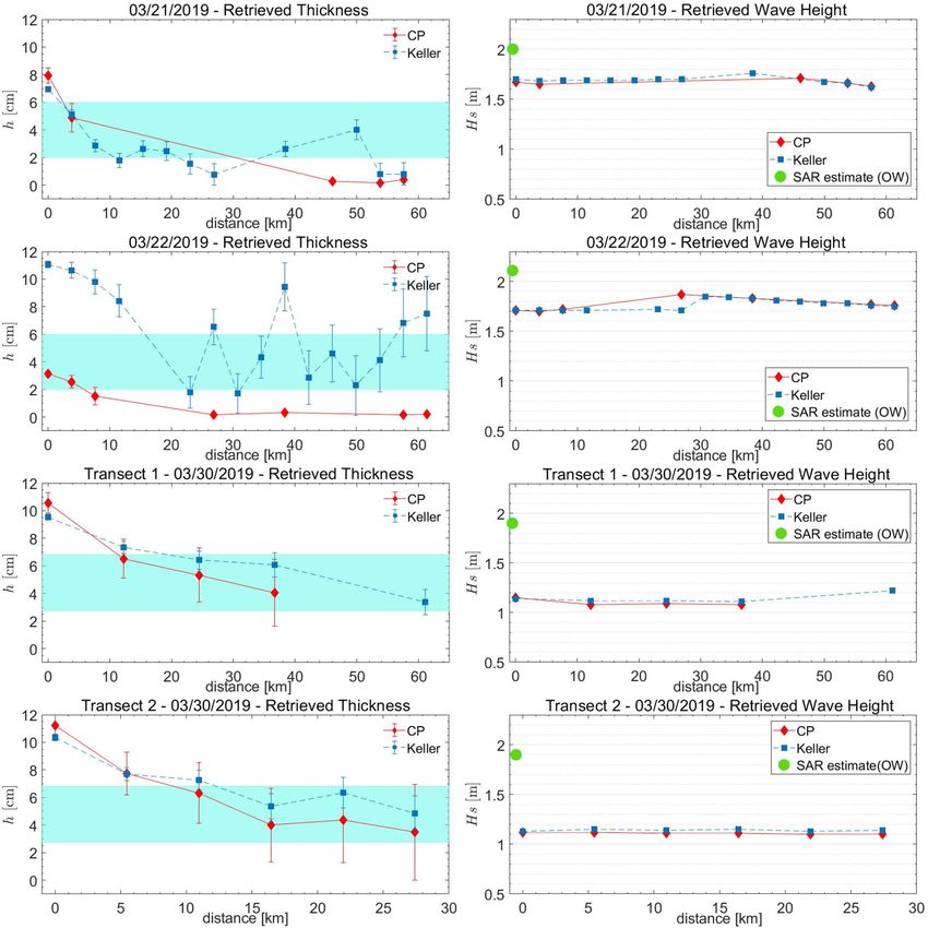
www.nature.com/scientificreports/
Figure 1. GPI viscosity versus equivalent thickness obtained by running Keller’s model (left panel) and CP
model (right panel), for the calibration instances selected from the ERS2 SAR images gathered in the Odden
region on 9 March and 11 March 1997, respectively. Viscosity values are given by the absolute minimum of the
odel30. The
SAR cost function corresponding to the equivalent ice thicknesses predicted by the ice salt-flux ice m
27
two red points represent the pure grease ice viscosity grown in laboratory . Cyan areas represent the regions of
95% confidence level for the best fit line obtained as Bayesian linear r egression33.
Figure 2. (A) Portion of the Sentinel-1A (S1A) IW-mode SAR image acquired on 1 November 2015 at
17:23 UTC in the Beaufort Sea. Representation is in the ground range/azimuth SAR acquisition reference
frame. Superimposed is the lat/lon grid. T1 (red), T2 (blue), and T3 (green) are the three transects selected
for ice thickness estimation around the corresponding points. The yellow pins indicate the location of ice
measurements made according to the ASSIST protocol within ±1 hour the SAR image data take; the black star is
the position of the wave buoy WB02 deployed during the field operations and operated to provide the wave field
at 17:30 UTC. The bright cross encircled by the yellow ring is the imaged R/V Sikuliaq. (B) Observed SAR image
wavenumber spectrum in open sea at 72.68◦ N 159.20◦ W. (C) Corresponding retrieved ocean wavenumber
directional spectrum.
βK = ηK g 1/2 h5/2 , βCP = ηCP g 1/2 h−3/2 . (8)
The dimensionless coefficient η can be evaluated by fitting the Odden data in Fig. 1:
ηK = 9.089 ± 0.516, ηCP = 0.963 ± 0.093. (9)
The smallness of the uncertainty in ηK and ηCP is an indication that the constitutive relation Eq. (7) provides a
physically reasonable description of the rheology of the ice layer. The difference between ηK and ηCP , however, is
striking. The most natural explanation for this phenomenon is that the viscosity in the Keller model refers to the
whole GPI mixture, while in the CP model it refers properly to grease ice layer. In fact, the CP model provides GPI
viscosities which are consistent with laboratory measurements27, while in the case of the Keller’s model the GPI
viscosity is about one order of magnitude higher than the laboratory measurements. We think that such higher
Scientific Reports | (2021) 11:2733 | https://doi.org/10.1038/s41598-021-82228-x 4
Vol:.(1234567890)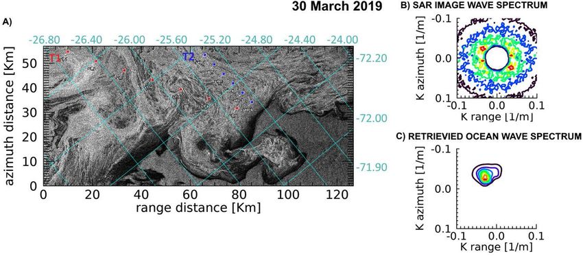
www.nature.com/scientificreports/
Observed SAR spectral parameters @ Retrieved SAR spectral parameters @ Retrieved ocean wave spectrum
Satellite peak location peak location parameters
Date/ Orbit/ Pixel size Value Wavelength Value Wavelength Wavelength
Time Sensor Band/Pol look (m) (arb. unit) (m) Dir. (deg) (arb. unit) (m) Dir. (deg) (m) Dir. (deg) Hs (m)
11/1/2015 DESC/
S1A C/HH 10 13 113 225 39 118 214 118 214 1.45
17:23 RIGHT
3/21/2019 DESC/
CSK1 X/VV 15 27 100 133 25 108 106 128 274 2.00
17:16 RIGHT
3/22/2019 DESC/
CSK4 X/VV 15 24 110 114 25 121 108 147 274 2.11
17:10 RIGHT
3/30/2019 ASC/
CSK4 X/VV 15 32 141 234 26 141 234 168 232 1.90
10:00 RIGHT
Table 1. Characteristics of the Sentinel-1A and COSMO-SkyMed SAR images selected for the application the
SAR inversion procedure to infer GPI thickness. Results of the best fit SAR image spectra at the peak location
along with the retrieved ocean wave spectra parameters in open sea are also reported.
viscosity, required to fit the data with the Keller’s model, reflects the contribution of pancakes to the overall ice
viscosity. Once the value of β from the cost function of the actual SAR inverted tile is available, the average ice
thickness of the GPI region travelled by the wave system can be computed from Eq. (9) into Eq. (8). The result is
2/5
h = (0.414 ± 0.009)g −1/5 βK (10)
for the Keller’s model, and
−2/3
h = (0.975 ± 0.064)g 1/3 βCP (11)
for the CP model, respectively. The uncertainty of β in Eqs. (10) and (11) is assumed negligible compared to
that of η.
Examples of SAR inferred GPI thicknesses. Equations (10) and (11) are imposed in the SAR-wave
inversion procedure that is applied to map the GPI thicknesses from a Sentinel-1A (S1A) SAR image gathered
in the Beaufort Sea, and from three COSMO-SkyMed (CSK) images collected in the Weddell Sea, Antarctica,
respectively. All details of SAR images are listed in Table 1.
Arctic‑Beaufort Sea. On 1 November 2015, an IW-mode S1A SAR image was collected in the advancing MIZ
of the Beaufort Sea (Fig. 2). At the time of SAR acquisition, the R/V Sikuliaq was in operation to carry out a field
cruise as part of a large collaborative program to study the coupled air-ice-ocean-wave processes occurring in
the Arctic during the autumn ice advance9.
A sharp ice edge can be detected in the S1A SAR image separating the open sea (bottom part) from the ice
field. The region of icefield directly exposed to open sea appears to be mainly composed of GPI. The hourly visual
observations conducted aboard the R/V Sikuliaq using the ASSIST protocol (http://www.iarc.uaf.edu/icewatch)
recognized three ice types, namely, young grey ice, pancakes and first year ice, along with an estimation of the
primary thickness and partial concentrations for each ice type. Occasional ship-side retrieval of frazil ice and
pancakes samples was also carried out as a concurrent measurement, and a number of directional wave buoys
were deployed.
At the time of SAR acquisition, a SWIFT wave buoy was floating in open sea around the ice edge, close to the
ship, where an incoming wave spectrum was measured with wave height HS ≃ 1.2 m. Figure 2, panel B, shows
the two-dimensional SAR image wavenumber spectrum observed by S1A in a 512 × 512 pixels open sea area,
centered at (72.68N, 159.20W), close to the ice edge and near to the SWIFT buoy location; the corresponding
two-dimensional directional ocean wave spectrum, shown in the panel C, is obtained using the SWIFT buoy wave
spectrum as first guess input12. The SAR inversion procedure returns a consistent wave directional spectrum,
with a slightly higher value of wave height HS ≃ 1.5 m (Table 1).
Following the dominant wave direction, three transects were selected, respectively formed by 13 (transect
1, T1), 15 (T2) and 11 (T3) SAR image tiles of size 256 × 256 pixels, as shown in Fig. 2. The retrieved ice thick-
nesses are shown in Fig. 3, along with the range of thicknesses from both the ASSIST protocol observations.
Results were also compared with the sea ice thickness retrieved from the L-band microwave sensor Soil Mois-
ture and Ocean Salinity (SMOS). Daily coverage of the polar regions with a resolution of about 35 km × 35 km
are indeed inferred through an empirical m ethod35 from SMOS acquisitions. It is worth to note that SMOS sea
ice thicknesses (cyan band in Fig. 3) underestimate the primary sea ice thicknesses from ASSIST protocol (grey
band in Figure 3).
Thicknesses from SAR retrievals using CP and Keller’s models are all within the SMOS and ASSIST range of
thicknesses and show a consistent behaviour running over the ice field depth. The overall trend shows increasing
thicknesses going from the ice edge up to values close to 25 cm.
In transect T1 a good agreement between CP and Keller results is observed. At the fourth location, close to
the ship, a thickness of 7.3 ± 2.9 cm from CP model and 8.7 ± 1.5 cm from Keller’s model are estimated, which
Scientific Reports | (2021) 11:2733 | https://doi.org/10.1038/s41598-021-82228-x 5
Vol.:(0123456789)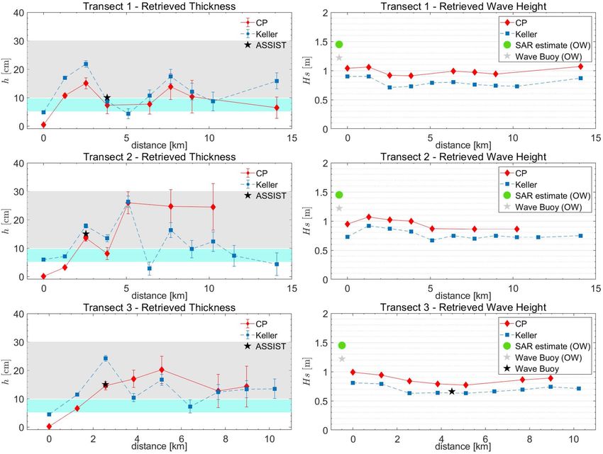
www.nature.com/scientificreports/
Figure 3. Estimated sea ice thicknesses (left column) and significant wave heights (right column) over the three
transects selected on the S1A SAR image using the Keller’s (blue dots) and CP model (red dots), respectively.
(left column) The cyan band represents the variability of the SMOS thicknesses in the area covered by the
transects. The grey band represents the range of thicknesses of the sea ice cover using the ASSIST protocol on
1 November. The black “star” symbol represents the primary thickness estimate using the ASSIST protocol
at the location of the corresponding SAR window within one hour the SAR acquisition. (right column) The
green circle indicates the significant wave height Hs estimated from SAR in open water; the grey “star” is the
concurrent measurement of Hs in open water from wave buoy S15, the black “star” is Hs measured by wave buoy
WB02 in the ice field. Wave buoy names are as indicated in the field campaign r eports9. WB02 location is signed
by a black star in Fig. 2A.
are consistent with the 10 cm of primary thickness from ASSIST estimation as well as with the average thickness
9.6 ± 3.8 cm obtained from pancake measurements collected in six recovery l ocations20.
In transect T2, thicknesses retrieved with both CP and Keller’s models agree for the first 5 km inside the
ice fields (windows 1–5). A good correspondence between ASSIST thickness (15 cm) and SAR retrievals (CP:
13.6 ± 1.2 cm; Keller: 17.8 ± 0.8 cm), at the third location, is again observed. From window 6 onward, the thick-
nesses inferred with the two models show different trends. This could be explained by inspecting the SAR image
in Fig. 2. In correspondence to window 6, a dark zone is indeed observed, which is consistent with grease ice
feature, possibly mixed with water, in the absence of pancakes. In such area wind can easily transfer energy to
waves, altering the attenuation trend by the GPI, measured up to window 5.
In this regard, we point out that the SAR inversion procedure compares the open water wave spectrum with
the wave spectrum observed at the specific window in sea ice. What the SAR procedure actually returns is there-
fore the average h∗n of the effective thickness h from the open sea to the given window,
1
n
h∗n = hi . (12)
n
i=1
In order to find the GPI thickness specific only for the window n, the contribution from the previous windows
has then to be removed as follows,
Scientific Reports | (2021) 11:2733 | https://doi.org/10.1038/s41598-021-82228-x 6
Vol:.(1234567890)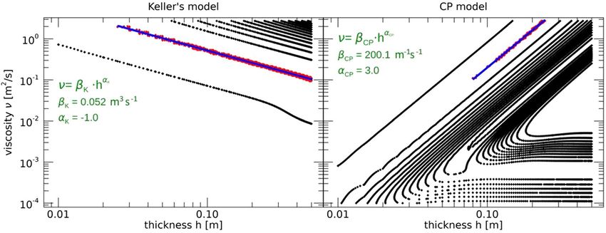
www.nature.com/scientificreports/
Figure 4. (A) Portion of the COSMO-SkyMed Wide Region mode SAR image acquired in the Weddell
Sea on 21 March 2019, represented in the geometry of the SAR acquisition reference frame. Superimposed
are the lat/lon grids. The aligned blue dots represent the locations along the transect T1 selected for ice
thickness estimation. (B) Observed SAR image wavenumber spectrum in open sea at (72.00 S, 27.15 W). C)
Corresponding retrieved wavenumber directional spectrum in open ocean.
hn = nh∗n − (n − 1)h∗n−1 . (13)
Negative values for hn can result. In this case, the data are not reported, as it happens for CP thickness estimation
of window 6 belonging to T2. Moreover, note that the CP model specifically represents a systems in which objects,
identified as pancakes or small ice floes, float upon a viscous layer, i.e. grease ice. A negative hi may therefore
indicate an absence of pancakes in the considered location, which could lead to wave build-up from wind action.
The two models return thickness values in the following windows of T2 that vary somewhat from window to
window, even though they remain in the range defined by the SMOS and ASSIST estimates. This difference in
thicknesses could reveal changes of the ice cover, which cannot longer be handled by the CP model.
Finally, as for T1, in transect T3, CP and Keller’s model infer comparable values of the thickness. Also in the
third location, there is good agreement between ASSIST thickness (15 cm) and CP thickness (14.6 ± 1.5 cm)
from SAR, but a slight disagreement with Keller’s thickness, which resulted as high as 24.2 ± 1.0 cm. Regarding
the SAR retrieved wave heights in sea ice, Fig. 3 shows consistent values for CP and Keller’s model. In particu-
lar, transect T3 intercepted the wave buoy WB02 about between window 7 and 8, as depicted in Fig. 2. WB02
measured a wave field of Hs ≈ 0.66 m. It is worth to note that the SAR analysis reported wave heights ranging
from 0.63 m at window 7 for the Keller’s model to 0.79 m at window 8 for the CP model, thus demonstrating the
effectiveness of the SAR inversion procedure in sea ice.
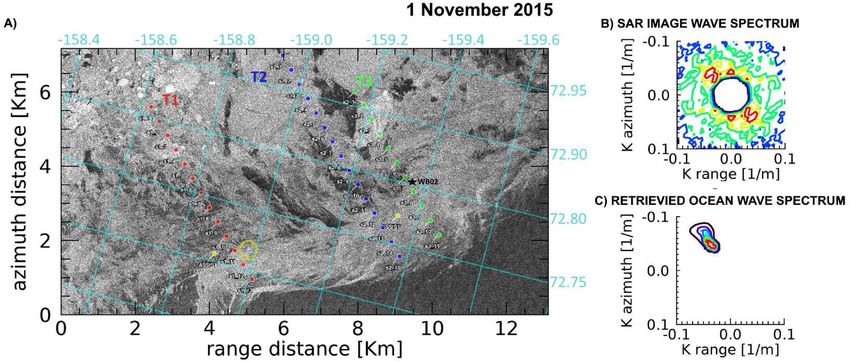
Antarctica‑Weddell Sea. In the context of the Year of Polar Prediction (YOPP) initiative of the World Meteoro-
logical Program36, a survey of the advancing ice edge of the Weddell Sea was performed during March 2019 by
exploiting the imaging capability of the four SAR satellites forming the COSMO-SkyMed (CSK) constellation.
We have applied the SAR-wave inversion technique to the SAR WIDEREGION images acquired on 21, 22 and
30 March 2019, where at least one CSK SAR satellite was able to image the sea ice edge.
An open ocean wave field of HS ≃ 2.0 m carrying dominant wavelengths ranging from ≃ 128 m to
≃ 168 m is observed to cross the GPI fields in the three dates. The associated wave spectra in open ocean
are obtained from SAR inversion using the closest 2D WAM s pectrum37 available for each date. Details of SAR
images characteristics and retrieved wave fields are listed in Table 1.
A common feature of the three SAR images is represented by the dark areas adjacent to the ice edge at direct
contact with the open sea, which reveal the presence of bands of pure frazil/grease ice, from which pancakes
originate. The SAR images taken on 21 and 22 March almost overlapped the same area of the Weddell Sea and
were able to image the outermost part of the developing GPI field; on 30 March, a wider area was imaged by
the SAR instrument, which includes the region imaged on 21 and 22 March, thus showing an expansion of the
GPI field. Figures 4, 5 and 6 show the interfaces separating open sea with the developed GPI fields imaged by
the CSK SAR images where the SAR-wave inversion procedure was applied. As for Fig. 2, transects are selected
approximately following the propagation of the dominant wave. For each location of the transects the estimated
thicknesses and the significant wave heights are plotted in Fig. 7 according to the distances inside the ice field.
The SMOS thicknesses over the area covered by the transects are also reported as band of variability.
As a general comment, smaller values of the thickness, much closer to the SMOS estimations, resulted from
the SAR inversion, compared to the Beaufort Sea case study. In the region closer to the ice edge the inferred GPI
thickness is about 3 cm higher the extremal SMOS value, with a trend to decrease when running towards the
Scientific Reports | (2021) 11:2733 | https://doi.org/10.1038/s41598-021-82228-x 7
Vol.:(0123456789)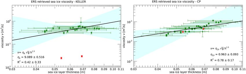
www.nature.com/scientificreports/

                                            Figure 5.  (A) Portion of the COSMO-SkyMed Wide Region mode SAR image acquired in the Weddell
                                            Sea on 22 March 2019, represented in the geometry of the SAR acquisition reference frame. Superimposed
                                            are the lat/lon grids. The aligned blue dots represent the locations along the transect T1 selected for ice
                                            thickness estimation. (B) Observed SAR image wavenumber spectrum in open sea at (72.00 S, 25.65 W). (C)
                                            Corresponding retrieved wavenumber directional spectrum in open ocean.

                                            Figure 6.  (A) Portion of the COSMO-SkyMed Wide Region mode SAR image acquired in the Weddell Sea on
                                            30 March 2019, represented in the geometry of the SAR acquisition reference frame. Superimposed are the lat/
                                            lon grids. The aligned red (blue) dots represent the locations along the transect T1 (T2) selected for ice thickness
                                            estimation. (B) Observed SAR image wavenumber spectra in open sea at (71.95 S, 25.92 W). (C) Corresponding
                                            retrieved wavenumber directional spectrum in open ocean.

                                            inside of the icefield, in contrast to the case study in the Arctic. The phenomenon could be caused by the action
                                            of the wave field that tends to compact the GPI in the region immediately surrounding the ice edge.
                                                Figures 4 and 5 show a very dynamic ice field with many darker areas of pure grease ice, and possibly water,
                                            embedded in the GPI environment. As occurred in transect T2 in Fig. 3, also in this case the CP model often
                                            appears unable to achieve thickness retrieval. It is worthwhile to note that for the 21st of March a general trend
                                            of decreasing thickness is obtained using both models, with comparable values of h, when available. Similarly,
                                            a general agreement between the inferred thicknesses is observed for the two transects of the 30th of March.

          Scientific Reports |   (2021) 11:2733 |                https://doi.org/10.1038/s41598-021-82228-x                                                   8

Vol:.(1234567890)
www.nature.com/scientificreports/
Figure 7. As for Figure 3 but relevant to the transects selected on the CSK SAR images acquired in March 2019.
Discussion
A new technique aimed at the estimation of GPI thickness from the inversion of SAR image wave spectra is
proposed. The intrinsic undetermination of any SAR inversion technique based on a viscous layer model is
resolved with an empirically determined constitutive relationship between the viscosity and the thickness of
the GPI layer, ν ∝ h3/2.
A similar power-law relation, ν ∝ h2, was proposed in38 on dimensional grounds, based on the hypothesis
that ν only depends on the wave frequency and the ice thickness. We point out that in our case h is an effective
thickness, proportional through Eq. (3) to the ice volume fraction. The ice volume fraction is expected to increase
with h under the effect of the buoyancy pressure39, which is itself proportional to the effective ice thickness h,
Ps ∼ �ρhg , where �ρ is the mass density gap between ice and liquid water. This gives a physical content to Eq.
(7), which goes well beyond the level of a dimensional relation. The microscopic justification of Eq. (7), however,
remains elusive, buried in the dependence of the dimensionless parameter η in Eq. (7) on internal GPI properties,
such as the geometry and size of frazil crystals and pancakes, and the water viscosity νw . We point out that any
dependence of η on νw , for dimensional consistency, would require dependence of η on an additional time scale,
which would require in turn dependence of η on g or other mechanical parameters, possibly associated with the
Scientific Reports | (2021) 11:2733 | https://doi.org/10.1038/s41598-021-82228-x 9
Vol.:(0123456789)www.nature.com/scientificreports/
stress in the ice matrix. In all cases, a picture of the GPI more akin to a brittle solid or a granular medium, than
to a fluid s uspension40, is suggested.
The prefactor in the constitutive equation is determined through a calibration procedure for two different
viscous layer models of wave propagation in GPI: the CP and the Keller’s model. To achieve the task, external
thickness information provided by the salt-flux model related to the 1997 Odden Ice T ongue30 are used as refer-
ence data.
The GPI viscosity-thickness relationship obtained for the CP model is comparable with the one found for
grease ice grown in wave tank at comparable thicknesses27. This is an encouraging result, as the CP model
assumes that viscous effects on wave propagation are due to grease ice only. On the other hand, the Keller’s
model envisions a layer of grease ice in which pancakes and small floes are suspended. Therefore, the resulting
effective viscosity is determined by all types of ice composing the ice layer. A physical interpretation for Eq. (9)
is possible following M ooney41. Indicating with φ the volume fraction of the pancakes (suspensions) and with
φc = π/6 ≈ 0.52 its value in the case of maximally packed spheres on the sites of cubic lattice, the effective
viscosity of the mixture, ν , should obey the following equation:
ν 2.5φ
ln = (14)
νgrease 1 − φ/φc
where for νgrease is taken the viscosity calibrated for CP. The values obtained for ηK and ηCP in Eq. (9) are compat-
ible with a layer in which the volume fraction of the pancakes is about φ = 0.33. This value of concentration is
physically sound and consistent with field measurements reported for the Weddell Sea in A ntarctica8.
The application of the two calibrated viscosities to different SAR images reveals that the inferred thicknesses
obtained by the two models are generally in good agreement, and agree with the other estimates of GPI thickness
available. The CP model seems to work better in real GPI fields, when both grease and pancake ice are present;
the Keller’s model seems more robust and to work well also in pancake free situations.
Methods
The SAR‑wave inversion procedure. The approach considers the ocean waves generated in open sea that
cross the ice edge and finally propagate in the icefield. It is assumed that the wave spectral features are modified
by the GPI cover through viscous interactions modeled either by the CP or Keller’s model. A SAR cost function is
defined to measure the distance between the observed SAR image spectrum and the one simulated as a function
of the wave models’ parameterization, i.e., ice thickness and viscosity.
SAR inversion in open ocean. The first step consists of the estimation of the directional open ocean wave spec-
trum at the boundary of the icefield from the available SAR image. The corresponding wavenumber SAR image
spectrum is estimated from a tile, typically 512 × 512 pixels in range and azimuth. If the single look complex
SAR image product is available, the SAR image cross-spectrum is calculated starting from the temporal separa-
tion between SAR looks, τ . SAR cross spectra significantly reduce the speckle noise level while preserving the
spectral shape, and provides information about the wave propagation d irection28. The simulated SAR image
spectrum is computed using the closed form expression of the non-linear ocean-to-SAR spectral form described
in Hasselmann and Hasselmann (1991)12 and later modified for the SAR image cross-spectral transform28. For
τ = 0 the SAR image cross-spectrum becomes a real-valued quantity and reduces to the standard multilooked
SAR image spectrum. According to the procedure proposed by Mastenbroek and De Valk (2000)42, the wind-
generated ocean spectrum is first estimated. The parametric representation given by Donelan et al. (1985)43 is
assumed, which depends on the inverse age of the dominant wave, � = U10 /cp , where U10 is the 10 m asl wind
speed and Cp is the phase velocity of the dominant wave, and the wind vector as well. The latter can be taken
either from in situ measurements, if available, or SAR-estimated using the wind vector from a numerical weather
prediction model, i.e. ECMWF, as first guess44. Then, the residual wave spectrum is estimated by assuming a
parametric representation of directional swells according to the JONSWAP-Glenn spectral shape coupled with
a directional spreading function of the Mitsuyasu type, properly extended for swell propagation45. This choice
accounts for non-linearity in SAR imaging features induced by high swells that can occur in the polar seas. Thus,
the implemented SAR retrieval of swells adopted a non-linear retrieval scheme which minimizes a cost function
with the truncated Newton method implemented in IDL©with respect to the following seven parameters: the
dominant wind wavenumber vector; the dominant swell wavenumber vector; the swell wave height; the shape
parameters and the directional spread of the swell distribution. The Hasselmann and Hasselmann (1991)12 inver-
sion method is applied in alternative, whenever the directional wave buoy data is available.
SAR inversion in the GPI field. A series of adjacent SAR tiles of 256 × 256 pixels centered at the position x
in the SAR reference frame and running from the ice edge along a straight line parallel to the direction of the
incoming dominant wave are selected through the GPI field. For each of them, the SAR image (cross-)spectrum
is computed. For the SAR images analyzed in this paper, the pixel sizes are 12.5 m for ERS2, 10 m for Sentinel-1A
and 15 m for COSMO-SkyMed SAR images. Thus, the spatial resolution of the final GPI thickness and viscosity
estimates is of the order of ≈ 10 km2.
It is assumed that the GPI cover alters the incoming ocean wave spectrum S̃w (k) as described in Eq. (1). For
each window located at position x into the SAR image, the SAR inversion scheme computes the waves-in-ice
spectrum that minimizes the cost function in Eq. (2). The integral definition of the cost function guarantees
that all the relevant contributions from the ocean spectrum are gathered through the corresponding SAR image
spectrum. After the ocean wave spectrum has been modified according to Eq. (1) through the selected wave
Scientific Reports | (2021) 11:2733 | https://doi.org/10.1038/s41598-021-82228-x 10
Vol:.(1234567890)www.nature.com/scientificreports/
model, the simulated SAR image spectrum is computed according to Hasselmann and H asselmann12 and Engen
and Johnsen28 for τ = 0. It is worth noting that application of the SAR inversion procedure requires the follow-
ing conditions to occur: (i) SAR imaging captures both open ocean and GPI, (ii) the wavefield is suitable for
SAR observation, and (iii) it is going toward the GPI. As the methodology requires accurate estimation of wave
attenuations to work properly, the incoming waves’ directions and the indentations of the ice edge as seen by
the SAR image are accounted for to allow accurate computation of the distances traveled by the waves from the
open sea to the point of observation.
The Keller’s and CP viscous wave propagation models. The two wave propagation models we con-
sider in our analysis assume that sea ice can be treated as a viscous medium. In the presence of gravity waves,
viscosity in the ice layer produces a finite normal stress on the ice-free water underneath, thereby modifying
the wave dispersion relation. The main difference between the Keller’s and the CP model resides in the way they
treat the contribution from pancakes. The Keller’s model implicitly treats GPI as homogeneous medium; the CP
model makes the hypothesis that pancakes lie on top of the grease ice layer. The pancake layer is supposed infi-
nitely thin in such a way that its only contribution to the wave dynamics is to generate a finite tangential stress at
the top of the grease ice layer. Such tangential stress is obviously absent in the case of the Keller’s model, where
the top of the ice layer corresponds to the interface with the atmosphere. In both models the normal stress at the
top of the ice layer is zero.
Both models assume a linear wave dynamics. In this regard, although there is evidence for a global increase of
typical ocean wave amplitudes2, possibly related to global climate change, a linear wave assumption still holds in
our analysis. Indeed in all cases here considered, the significant wave height is two orders of magnitude smaller
than the peak wavelength (see Table 1).
The tangential stress at the top of the ice layer is controlled in the CP model by a parameter which allows to
interpolate between a pancake free situation (corresponding to the Keller model) and a situation in which the
pancakes are so closely packed to form an inextensible layer.
The latter regime is the one which concerns us; field measurements b y46 support the modelling assumption.
In this regime both the Keller’s and the CP model are described by just two parameters: the thickness h of the
ice layer, and an effective ice viscosity ν which in the case of the CP model refers just to grease ice and in the case
of the Keller’s model refers to the whole GPI mixture. It is convenient to introduce the following dimensionless
parameters:
3/2 1/4
k∞ k∞ g 1/4
ν̂ = ν, ψ= h, (15)
g 1/2 ν 1/2
where k∞ = ω2 /g represents the wave number in open ocean and g = 9.8m/s2 the gravitational acceleration.
We can express the two parameters ν̂ and ψ in terms of the wavenumber k, the ice thickness h and the viscous
boundary layer depth α = (ω/ν)1/2, as ν̂ = (k α )1/2 and ψ = h/ α. We thus see that small ν̂ and ψ correspond
to a small ice contribution to the wave dynamics; in our analysis ν̂ ranges from 10−5 to 10−1 and ψ ranges from
10−2 to 10−1.
For small ν̂ and ψ , the dispersion relations for the CP and the Keller’s model take a very simple form,
2 i 1/2 5/2 h3
CP : k ≈ k∞ + ρ̂hk∞ + g k∞ 3 , (16)
ρ̂ ν
7/2
ρ̂k∞
Keller : k ≈ k∞ + 4i hν. (17)
g 1/2
where ρ̂ ≈ 0.92 is the ratio between the GPI density and the ocean water density. We can identify in Eq. (16)
a dispersion contribution that reproduces the result by the mass-loading model10. The wave attenuation is the
imaginary part of the wavenumber vector, q = I(k), that has in the two cases the simple power law form q ∝ h3 /ν
(CP model) and q ∝ hν (Keller’s model).
The h-dependence of ν in Eqs. (16) and (17) can be made explicit by applying the calibration results in Eqs.
(7) and (9):
2 iρ̂ 5/2 3/2
CP : k ≈ k∞ + ρ̂hk∞ + k h , (18)
3ηCP ∞
7/2 5/2
Keller : k ≈ k∞ + 4iρ̂ηK k∞ h . (19)
Geometric structure of the cost function minima. For small h the asymptotic relations Eqs. (16) and (17) can be
rewritten as
q(h, ν; ω) = A(h, ν)B(ω), (20)
where for the Keller’s model
Scientific Reports | (2021) 11:2733 | https://doi.org/10.1038/s41598-021-82228-x 11
Vol.:(0123456789)www.nature.com/scientificreports/
Figure 8. Exemplary contour plots of the cost functions obtained from SAR inversion in GPI field for the
Keller’s model (left panel) and the CP model (right panel). Red points mark those locations (h, ν) where the
cost function values are within 1% of the corresponding absolute minimum. This example corresponds to the
window number 13 selected on the ERS2 SAR image of the 9 March 1997 and is representative for any cases
considered in this paper.
7/2
ρ̂k∞ (ω)
A(h, ν) = hν, B(ω) = 4 , (21)
g 1/2
and for the CP model
5/2
h3 ρ̂g 1/2 k∞ (ω)
A(h, ν) = , B(ω) = . (22)
ν 3
Substituting Eq. (20) into Eq. (1) yields
Si (x, k∞ ; h, ν) = S̃w (k∞ ) exp[−2A(h, ν)B(ω(k∞ ))�(ek , x)], (23)
which tells us that the cost function in Eq. (2) depends on the variables h and ν only through A(h, ν):
�(τ , x; h, ν) = �(τ , x; A(h, ν)). (24)
The minimum of the cost function is determined by imposing
∂�
0 = ∇ν,h � = ∇ν,h A,
∂A
whose solution can be written in the form
Amin (ν, h) = F(τ , x). (25)
Combining Eqs. (21), (22) and (25) then yields Eqs. (4) and (5).
Although the above procedure can only be justified in the limit of small h, we verify that the result in Eqs.
(4) and (5) continues to hold for realistic values of h. The contour lines in Fig. 8 are obtained by simulating the
SAR image wave spectrum with the full wave dispersion relation. As this trend is common to all the examined
cases, we assume that Eq. (4) always holds.
Received: 30 July 2020; Accepted: 3 January 2021
References
1. Thomson, J. & Rogers, W. E. Swell and sea in the emerging arctic ocean. Geophys. Res. Lett. 41, 3136–3140 (2014).
2. Squire, V. A. Ocean wave interactions with sea ice: a reappraisal. Annu. Rev. Fluid Mech. 52, (2020).
3. Martin, S. Frazil ice in rivers and oceans. Annu. Rev. Fluid Mech. 13, 379–397 (1981).
4. Newyear, K. & Martin, S. A comparison of theory and laboratory measurements of wave propagation and attenuation in grease
ice. J. Geophys. Res. Oceans 102, 25091–25099 (1997).
5. Smedsrud, L. H. & Skogseth, R. Field measurements of arctic grease ice properties and processes. Cold Reg. Sci. Technol. 44, 171–183
(2006).
6. Leonard, G., Shen, H., Ackley, S., Shen, H. & Balkema, A. Dynamic growth of a pancake ice cover. In Ice in surface waters: Proceed‑
ings of the 14th International IAHR Ice Symposium, edited by: Shen, HT, Taylor & Francis, Rotterdam, ISBN, vol. 90, 9718 (1998).
7. Wadhams, P. & Wilkinson, J. The physical properties of sea ice in the odden ice tongue. Deep Sea Res. Part II 46, 1275–1300 (1999).
8. Doble, M. J., Coon, M. D. & Wadhams, P. Pancake ice formation in the weddell sea. J. Geophys. Res. Oceans 108, (2003).
Scientific Reports | (2021) 11:2733 | https://doi.org/10.1038/s41598-021-82228-x 12
Vol:.(1234567890)www.nature.com/scientificreports/
9. Thomson, J. et al. Overview of the arctic sea state and boundary layer physics program. J. Geophys. Res. Oceans 123, 8674–8687
(2018).
10. Peters, A. The effect of a floating mat on water waves. Commun. Pure Appl. Math. 3, 319–354 (1950).
11. Keller, J. B. Gravity waves on ice-covered water. J. Geophys. Res. Oceans 103, 7663–7669 (1998).
12. Hasselmann, K. & Hasselmann, S. On the nonlinear mapping of an ocean wave spectrum into a synthetic aperture radar image
spectrum and its inversion. J. Geophys. Res. Oceans 96, 10713–10729 (1991).
13. Wadhams, P. & Holt, B. Waves in frazil and pancake ice and their detection in seasat synthetic aperture radar imagery. J. Geophys.
Res. Oceans 96, 8835–8852 (1991).
14. Wadhams, P., De Carolis, G., Parmiggiani, F. & Tadross, M. Wave dispersion by frazil-pancake ice from sar imagery. In IGARSS’97.
1997 IEEE International Geoscience and Remote Sensing Symposium Proceedings. Remote Sensing-A Scientific Vision for Sustainable
Development, vol. 2, 862–864 (IEEE, 1997).
15. Wadhams, P., Parmiggiani, F. & De Carolis, G. The use of sar to measure ocean wave dispersion in frazil-pancake icefields. J. Phys.
Oceanogr. 32, 1721–1746 (2002).
16. Wadhams, P., Parmiggiani, F., De Carolis, G. & Tadross, M. Mapping the thickness of pancake ice using ocean wave dispersion in
sar imagery. In Oceanography of the Ross Sea Antarctica, 17–34 (Springer, 1999).
17. De Carolis, G. Retrieval of the ocean wave spectrum in open and thin ice covered ocean waters from ERS synthetic aperture radar
images. Nuovo Cimento. C 24, 53–66 (2001).
18. De Carolis, G. SAR measurements of directional wave spectra in viscous sea ice. Rivista Italiana di Telerilevamento 26, 31–36
(2003).
19. Wadhams, P., Parmiggiani, F., De Carolis, G., Desiderio, D. & Doble, M. SAR imaging of wave dispersion in Antarctic pancake ice
and its use in measuring ice thickness. Geophys. Res. Lett. 31, (2004).
20. Wadhams, P., Aulicino, G., Parmiggiani, F., Persson, P. & Holt, B. Pancake ice thickness mapping in the Beaufort sea from wave
dispersion observed in SAR imagery. J. Geophys. Res. Oceans 123, 2213–2237 (2018).
21. Doble, M. J., De Carolis, G., Meylan, M. H., Bidlot, J.-R. & Wadhams, P. Relating wave attenuation to pancake ice thickness, using
field measurements and model results. Geophys. Res. Lett. 42, 4473–4481 (2015).
22. De Carolis, G. & Desiderio, D. Dispersion and attenuation of gravity waves in ice: a two-layer viscous fluid model with experimental
data validation. Phys. Lett. A 305, 399–412 (2002).
23. Wang, R. & Shen, H. H. Gravity waves propagating into an ice-covered ocean: A viscoelastic model. J. Geophys. Res. Oceans 115,
(2010).
24. Cheng, S. et al. Calibrating a viscoelastic sea ice model for wave propagation in the arctic fall marginal ice zone. J. Geophys. Res.
Oceans 122, 8770–8793. https://doi.org/10.1002/2017JC013275 (2017).
25. De Santi, F. et al. On the ocean wave attenuation rate in grease-pancake ice, a comparison of viscous layer propagation models
with field data. J. Geophys. Res. Oceans 123, 5933–5948 (2018).
26. De Santi, F. & Olla, P. Effect of small floating disks on the propagation of gravity waves. Fluid Dyn. Res. 49, 025512 (2017).
27. Newyear, K. & Martin, S. Comparison of laboratory data with a viscous two-layer model of wave propagation in grease ice. J.
Geophys. Res. Oceans 104, 7837–7840 (1999).
28. Engen, G. & Johnsen, H. Sar-ocean wave inversion using image cross spectra. IEEE Trans. Geosci. Remote Sens. 33, 1047–1056
(1995).
29. Sutherland, P. & Gascard, J.-C. Airborne remote sensing of ocean wave directional wavenumber spectra in the marginal ice zone.
Geophys. Res. Lett. 43, 5151–5159 (2016).
30. Pedersen, L. T. & Coon, M. D. A sea ice model for the marginal ice zone with an application to the greenland sea. J. Geophys. Res.
Oceans 109, (2004).
31. Holland, P. R. et al. Modeled trends in Antarctic sea ice thickness. J. Clim. 27, 3784–3801 (2014).
32. Liu, Q., Rogers, W. E., Babanin, A., Li, J. & Guan, C. Spectral modeling of ice-induced wave decay. J. Phys. Oceanogr. 50, 1583–1604
(2020).
33. Kelly, B. C. Some aspects of measurement error in linear regression of astronomical data. Astrophys. J. 665, 1489 (2007).
34. Newyear, K. & Martin, S. Comparison of laboratory data with a viscous two-layer model of wave propagation in grease ice. J.
Geophys. Res. (Ocean) 104, 7837–7840 (1999).
35. Huntemann, M. et al. Empirical sea ice thickness retrieval during the freeze up period from SMOS high incident angle observa-
tions. Cryosphere 8, 439–451 (2014).
36. Jung, T. et al. Advancing polar prediction capabilities on daily to seasonal time scales. Bull. Am. Meteorol. Soc. 97, 1631–1647
(2016).
37. Janssen, P. A. E. M. The wave model (ECMWF, 2002).
38. Sutherland, G., Rabault, J., Christensen, K. H. & Jensen, A. A two layer model for wave dissipation in sea ice. Appl. Ocean Res. 88,
111–118 (2019).
39. Olla, P. Mechanical diffusion in grease ice stirred by gravity waves. Fluid Dyn. Res. 50, 045503 (2018).
40. De Carolis, G., Olla, P. & Pignagnoli, L. Effective viscosity of grease ice in linearized gravity waves. J. Fluid Mech. 535, 369–381
(2005).
41. Mooney, M. The viscosity of a concentrated suspension of spherical particles. J. Colloid Sci. 6, 162–170 (1951).
42. Mastenbroek, Cd. & De Valk, C. A semiparametric algorithm to retrieve ocean wave spectra from synthetic aperture radar. J.
Geophys. Res. Oceans 105, 3497–3516 (2000).
43. Donelan, M. A., Hamilton, J. & Hui, W. Directional spectra of wind-generated ocean waves. Philos. Trans. R. Soc. Lond. Ser. A.
Math. Phys. Sci. 315, 509–562 (1985).
44. Portabella, M., Stoffelen, A. & Johannessen, J. A. Toward an optimal inversion method for synthetic aperture radar wind retrieval.
J. Geophys. Res. Oceans 107, 1 (2002).
45. Goda, Y. Random seas and design of maritime structures (World Scientific, Singapore, 2010).
46. Smith, M. & Thomson, J. Pancake sea ice kinematics and dynamics using shipboard stereo video. Ann. Glaciol. 1–11, (2019).
Acknowledgements
This work was part of the project “WAMIZ-Waves in the Ice” funded by the Italian PNRA (Grant PNRA18_00109).
This is also a contribution to the Year of Polar Prediction (YOPP), a flagship activity of the Polar Prediction Pro-
ject (PPP), initiated by the World Weather Research Programme (WWRP) of the World Meteorological Organisa-
tion (WMO). We acknowledge the WMO WWRP for its role in coordinating this international research activity.
We also acknowledge the activity carried out in the FP7 EU project ICE-ARC (Grant Agreement 603887). The
Project was carried out using CSK®Products ©ASI (Italian Space Agency), delivered under the ASI licence to
use ID 714 in the framework of COSMO-SkyMed Open Call for Science. The Sentinel-1A used in this work was
freely delivered by ESA through the Copernicus Open Access Hub (https: //scihub .copern icus. eu/dhus/#/home).
Scientific Reports | (2021) 11:2733 | https://doi.org/10.1038/s41598-021-82228-x 13
Vol.:(0123456789)www.nature.com/scientificreports/
Author contributions
G.D.C. SAR processing; G.D.C., F.D.S. data analysis; F.D.S., P.O. theoretical models. The results were discussed
and interpreted by all authors. All authors contributed to write the manuscript.
Competing interests
The authors declare no competing interests.
Additional information
Correspondence and requests for materials should be addressed to G.D.C.
Reprints and permissions information is available at www.nature.com/reprints.
Publisher’s note Springer Nature remains neutral with regard to jurisdictional claims in published maps and
institutional affiliations.
Open Access This article is licensed under a Creative Commons Attribution 4.0 International
License, which permits use, sharing, adaptation, distribution and reproduction in any medium or
format, as long as you give appropriate credit to the original author(s) and the source, provide a link to the
Creative Commons licence, and indicate if changes were made. The images or other third party material in this
article are included in the article’s Creative Commons licence, unless indicated otherwise in a credit line to the
material. If material is not included in the article’s Creative Commons licence and your intended use is not
permitted by statutory regulation or exceeds the permitted use, you will need to obtain permission directly from
the copyright holder. To view a copy of this licence, visit http://creativecommons.org/licenses/by/4.0/.
© The Author(s) 2021
Scientific Reports | (2021) 11:2733 | https://doi.org/10.1038/s41598-021-82228-x 14
Vol:.(1234567890)You can also read