Compact Current Source Models for Timing Analysis under Temperature and Body Bias Variations
←
→
Page content transcription
If your browser does not render page correctly, please read the page content below

IEEE TRANSACTIONS ON VERY LARGE SCALE INTEGRATION (VLSI) SYSTEMS                                                                            1

                      Compact Current Source Models
                         for Timing Analysis under
                    Temperature and Body Bias Variations
                                       Saket Gupta, and Sachin S. Sapatnekar, Fellow, IEEE,

   Abstract—State-of-the-art timing tools are built around the               load capacitance [4]. When interconnect resistance became
use of current source models (CSMs), which have proven to be                 significant, these methods were replaced by the notion of
fast and accurate in enabling the analysis of large circuits. As             effective capacitance [5]. However, this approach models the
circuits become increasingly exposed to process and temperature
variations, there is a strong need to augment these models to                input as a saturated ramp with piecewise constant slope, and
account for thermal effects and for the impact of adaptive body              was further enhanced by the development of CSMs, which
biasing, a compensatory technique that is used to overcome on-               represent a cell as a voltage controlled current source and
chip variations. However, a straightforward extension of CSMs                provide fast and accurate timing estimates.
to incorporate timing analysis at multiple body biases and                      A CSM approach termed as “Blade” [6] represents the
temperatures results in unreasonably large characterization tables
for each cell. We propose a new approach to compactly capture                cell as a voltage-controlled current source (VCCS) with an
body bias and temperature effects within a mainstream CSM                    internal capacitance and a time-shifted input waveform driving
framework. Our approach features a table reduction method for                an arbitrary load. A lookup table, indexed by the input voltage,
compaction of tables and a fast and novel waveform sensitivity               Vin , and the output voltage, Vout , models the VCCS current,
method for timing evaluation under any body bias and temper-                 Iout . These ideas were further refined in [7]–[12]. The work
ature condition. On a 45nm technology, we demonstrate high
accuracy, with mean errors of under 4% in both slew and delay                in [7], [8] removed the assumptions of linearity, and [9]–[12]
as compared to HSPICE. We show a speedup of over five orders                 addressed multiple input switching and stack effects. Further,
of magnitude over HSPICE and a speedup of about 92× over                     a current source model based on orthogonal functions was
conventional CSMs.                                                           proposed in [13], and an approach based on the small-signal
                                                                             model of a transistor was built in [14].
                       I. INTRODUCTION                                          Within the CSM framework, process variations are com-
                                                                             monly captured through the use of process corners. Tradition-

V      ARIATIONS in process parameter values and on-chip
       temperatures have grown larger with shrinking feature
sizes. Process variations occur due to phenomena such as
                                                                             ally, temperature variations were also handled using corner-
                                                                             based methods, but this is no longer viable. Corner-based
                                                                             approaches are predicated on the idea that the timing varies
proximity effects in photolithography, non-uniform conditions                monotonically over the temperature range, but this is no longer
during deposition, and random dopant fluctuations, and lead                  the case with thermally-driven variations [15]. In nanometer-
to fluctuations in parameters such as transistor dimensions,                 scale technologies, elevated temperatures cause reductions in
oxide thicknesses, and dopant concentrations [1]–[3]. On-                    device mobilities (which tend to increase the delay) as well
chip temperature variations occur due to power dissipation in                as reductions in threshold voltages (which tend to decrease
the form of heat. Such thermal variations have a significant                 the delay). The interplay between these effects may cause the
bearing on the mobilities of electrons and holes, as well as                 circuit delay to increase monotonically (negative temperature
the threshold voltage of the devices. These effects have led                 dependence), decrease monotonically (positive temperature
to increased shifts in circuit performance, due to which a                   dependence), or vary nonmonotonically (mixed temperature
significant fraction of the total number of acceptable dies may              dependence) with temperature. In the last case, the worst case
fail to achieve the prescribed performance goals. To overcome                may occur in the interior of the temperature range, rather
this problem, designers must build resilient circuits that meet              than at its edges. As a result, a set of temperature corners
their performance goals in spite of these variations.                        is no longer adequate, and circuit delays must be simulated as
   A key enabler for variation-tolerant design is the ability                functions of temperature.
to simulate the timing behavior of a circuit during the de-                     Therefore, a first necessary enhancement of CSMs involves
sign process using static timing analysis (STA). Traditional                 extending them to determine the cell delay as a function
standard cell modeling approaches represent the delay and                    of temperature. This capability is useful not only for circuit
output slew as nonlinear functions of the input slew and output              analysis but also for building optimization techniques that
  Manuscript received October 18, 2010; revised August 01, 2011. This work   compensate for temperature variations [3], [16]–[19].
was supported in part by the SRC under contract 2007-TJ-1572 and by the         A second way in which CSMs require augmentation is in
NSF under award CCF-1017778.                                                 building an ability to simulate cell timing in the presence of
  The authors are with the Department of Electrical and Computer Engi-
neering, University of Minnesota, Minneapolis MN, 55455, USA (e-mail:        body biases. The application of adaptive body biases (ABBs)
saket@umn.edu)                                                               allows circuits to be made resilient and variation-tolerant by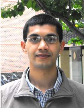
IEEE TRANSACTIONS ON VERY LARGE SCALE INTEGRATION (VLSI) SYSTEMS                                                                       2

applying a deliberate bias to the body terminals of transistors      We develop a scheme for characterizing this perturbation and
in a circuit. Realistically, ABB is applied at coarse levels of      computing it efficiently. Specifically, mathematical models for
granularity, e.g., by biasing individual n-wells and/or p-wells,     such parameters are developed and further analyzed for their
each of which contains a number of transistors. Forward body         independence over body bias and temperature variations for an
bias (FBB) effectively reduces the transistor threshold voltage      efficient computation of such parameters.
and speeds up the device, at the cost of increased leakage, while       The remainder of the paper is organized as follows. Sec-
reverse body bias (RBB) achieves the opposite effect on speed        tion II presents the development of sensitivity models for CSM
and leakage. ABB involves the use of FBB or RBB to help dies         components to handle variations in body bias and temperature.
recover from variations, and may be applied dynamically to           Section III presents our algorithms for compacting the CSM
tighten the distribution of the dies with maximum operational        sensitivity tables. Then we present the conventional macro-
frequency, while simultaneously meeting the leakage power            model solvers used in state-of-the-art CSMs in Section IV,
constraints [1]–[3], [17], [20].                                     and is followed by a description of our method for fast output
   Traditional CSMs simulate the circuit at fixed values of          waveform evaluation in Section V. Section VI presents exper-
the body bias (vbp = vbn = 0) and at fixed values of the             imental results on a set of library cells in a 45nm technology.
temperature. The obvious extensions to existing CSMs that            We then present the conclusion of our work in Section VII.
enable them to capture body biases and temperature effects
are rather inefficient. In principle, the body terminal of a            II. CSM SENSITIVITY MODEL DEVELOPMENT
device can be considered to be another port, and the cell
can be accordingly characterized by creating a look-up table
for various combinations of body biases, vbp , vbn . Further,
such lookup tables would have to be constructed for various
temperature values. However, this increases the amount of
memory used as well as the characterization time significantly
over the zero body bias and the nominal temperature case. For
instance, for 10 values each of vbp and vbn , and for 10 values
of temperature, the table for each library cell becomes 1000×
larger. The need to access a larger lookup table may also result     Fig. 1: Example of a CSM: the output port is modeled as
in a significant concomitant increase in the simulation runtime      a nonlinear VCCS dependent on all input port voltages, in
of CSM macromodels.                                                  parallel with a nonlinear capacitance.
   This paper develops efficient timing characterization meth-
ods for building CSMs that incorporate changes in the body              The CSM is a gate-level black-box abstraction of a cell in a
bias and the temperature. Since ABB is applied at the granu-         library, with the same input and output ports as the original cell.
larity of a well, we assume that all PMOS transistors in a cell      Our CSM structure, shown in Figure 1, is of the type proposed
have the same body bias value, vbp , and all NMOS devices are        in [6], and is augmented to model nonlinearities as in [9].
biased at vbn . Further we assume that all transistors in the cell   Specifically, output port p is replaced by a nonlinear voltage-
experience a uniform temperature: this is reasonable, since the      controlled-current-source (VCCS), Ip , in parallel with a non-
rate of decay of temperature with respect to the distance from       linear capacitance, Cp . The VCCS model enables the CSM
the cell has a “time constant” that is significantly larger than     to be load-independent, and permits it to handle an arbitrary
the size of a cell.                                                  electrical waveform at its inputs. The CSM is characterized
                                                                     in terms of the value of Ip and the charge, Qp , stored on
   Our framework for incorporating effects of body bias and
                                                                     the capacitor, Cp . The variables, Ip and Qp , are functions of
temperature into the CSM has a very small memory and
                                                                     all input and output port voltages and temperature, and are
runtime overhead, while maintaining high levels of accu-
                                                                     determined by characterizing the cell at various port voltages,
racy. Our mathematical framework consists of two key steps.
                                                                     body bias combinations and temperatures as follows:
First, we intelligently adapt an existing scheme to enable the
compaction of look-up tables for the sensitivities of CSM                            Ip   =    F (Vi , Vo , vbp , vbn , ∆T )        (1)
components to body bias and temperature, over the range                             Qp    =    G(Vi , Vo , vbp , vbn , ∆T )         (2)
of allowable values of both the applied body bias and on-
chip temperature. Our second key contribution is to develop          The parameters Ip and Qp are modeled using the functions
a novel waveform sensitivity model for evaluating the impact         F and G, respectively, and Vi and Vo are, respectively, the
of the applied body bias and variations in temperature, which        voltages at the transitioning input and output ports of the cell.
provides accurate waveforms at the output of the cell under any      We use the term ∆T to represent the temperature offset from a
body bias or temperature condition, with minimal computation.        baseline temperature value, taken here to be room temperature
The essential idea of this approach is that since body bias          (25◦ C). In the temperature range of [−25◦ C, 125◦ C] that we
or temperature variation constitutes a small perturbation to         work in, the range for the values of ∆T is [−50◦ C, 100◦ C].
the nominal waveform, it should be possible to determine the           For a cell, Ip characterization involves DC simulations over
perturbed waveform cheaply by determining and saving the             multiple combinations of DC values of (Vi , Vo ), while Qp is
parameters that compute its shift from the nominal waveform.         characterized through a set of transient simulations [9]. The
IEEE TRANSACTIONS ON VERY LARGE SCALE INTEGRATION (VLSI) SYSTEMS 3
presentation of our model is targeted to the more widely- all (Vi , Vo ) points. The CSM is now modified by using the
used scenario of single-input switching for gates with a single equations:
output, though the idea can easily be extended to multiple input
Ip (Vi , Vo ,vbp , vbn , 0)
switching (MIS) and multioutput gates, leveraging current work
on CSMs on these topics [9], [11], [12]. = IpZ · (1 + aI (Vi , Vo )vbp + bI (Vi , Vo )vbn ) (4)
As mentioned earlier, in order to capture the sensitivity of Qp (Vi , Vo ,vbp , vbn , 0)
CSM parameters to the applied body bias and temperature = QZ
p · (1 + aQ (Vi , Vo )vbp + bQ (Vi , Vo )vbn ) (5)
offset, in principle, the circuit could be characterized over a set
S of all possible (vbp , vbn , ∆T ) points, treating body terminals where IpZ = F (Vi , Vo , 0, 0, 0), QZ p = G(Vi , Vo , 0, 0, 0), and
as input ports, and temperature offset as the independent vari- {aI , bI , aQ , bQ } correspond to the sensitivity of the function
able. Since the allowable values of the applied body biases and to the corresponding body bias. These parameters are charac-
temperature offset change in discrete steps, the cardinality of terized at a discrete set of (Vi , Vo ) values and are saved in a
this set is large, and the corresponding characterization would lookup table.
be computationally intensive, even as a precharacterization The characterization of Ip and Qp using equations (4)
step that is to be performed once for a technology. Moreover, and (5) can now be carried out using a minimum of three
memory requirements of the table multiply significantly over simulations at each (Vi , Vo ), since it is a linear model; however,
the current characterization procedure at zero body bias and additional redundancy is preferable to account for the small
zero temperature offset. nonlinearities, and a linear least squares fit can be used instead.
We observe through simulations that the functions F and G For notational simplicity, we will define the following func-
depend much more weakly on vbp , vbn , and ∆T as compared to tions:
Vi or Vo . Hence, a simpler model can be utilized to save on this
LI (vbp , vbn ) = 1 + aI (Vi , Vo )vbp + bI (Vi , Vo )vbn (6)
computation. We thus develop sensitivity models of CSM with
respect to vbp , vbn and ∆T (as we will soon show, the models LQ (vbp , vbn ) = 1 + aQ (Vi , Vo )vbp + bQ (Vi , Vo )vbn (7)
with respect to body bias and temperature are independent), Clearly,
and then present a scheme to incorporate the effects of the
two. Ip (Vi , Vo , vbp , vbn , 0) = IpZ LI (vbp , vbn ) (8)
Qp (Vi , Vo , vbp , vbn , 0) = QZ
p LQ (vbp , vbn ) (9)
A. Independence of Body Bias and Temperature Effects
Next, we explain the rationale for analyzing the effects of C. CSM Temperature Sensitivity Model
body bias and temperature independently. Body bias (a change We now construct the temperature sensitivity model at zero
in the substrate bias voltage, VBS ) changes the threshold body bias. We observe that the variations of Ip and Qp
voltage, Vth . The sensitivity of Vth with respect to VBS can with ∆T are nonlinear, unlike the body bias case where a
be captured from following equation [21]: linear approximation was adequate. We employ a second-
∂Vth Cdep order polynomial approximation, and find that the fit has an
= (3) average relative error of 1.6% relative error in comparison with
∂VBS Cox
HSPICE simulations. The CSM for the temperature sensitivity
where Cdep is the depletion capacitance of the MOS transistor
model with the first and second order sensitivities in tem-
and Cox is the oxide capacitance. Cdep is a very weak function
perature offset is now represented by the following modified
of temperature, being proportional to the inverse square root
equations:
of the built-in potential. Similarly, it is observed that the
expression for Vth sensitivity with respect to temperature is Ip (Vi , Vo , 0, 0, ∆T )
independent of VBS [21]. Hence, the effects of changes in body = IpZ · (1 + cI (Vi , Vo )∆T + rI (Vi , Vo )∆T 2 ) (10)
bias and temperature on MOS transistors can be treated as in-
Qp (Vi , Vo , 0, 0, ∆T )
dependent. Since Ip and Qp essentially abstract the internal cell
behavior, the effects of body bias and changes in temperature = QZ 2
p · (1 + cQ (Vi , Vo )∆T + rQ (Vi , Vo )∆T ) (11)
on Ip and Qp can also be assumed to be independent. This is where IpZ , QZ p are as defined above, and {cI , cq , rI , rQ } cor-
further verified by the model formulations and accuracy results respond to the sensitivity of the function to the corresponding
as presented in the subsequent subsections and sections. powers of the temperature offset, ∆T . As in the case of {aI ,
bI , aQ , bQ }, these parameters are characterized at a discrete
B. CSM Body Bias Sensitivity Model set of (Vi , Vo ) values and saved in a lookup table. Since the
We first present the body bias sensitivity model, which is temperature sensitivity model is a second order model, we need
independent of the changes in temperature and constructed at least three points to determine the values of {cI , rI , cQ , rQ }.
at ∆T = 0◦ C (i.e., at room temperature). We construct a As before, for notational simplicity, we will define the
polynomial approximation for the variations of Ip and Qp following functions:
with respect to (vbp , vbn ). Our simulations show that a linear
SI (∆T ) = 1 + cI (Vi , Vo )∆T + rI (Vi , Vo )∆T 2 (12)
approximation yields an average of 2.0% relative error with 2
respect to HSPICE, evaluated over all (vbp , vbn ) points, for SQ (∆T ) = 1 + cQ (Vi , Vo )∆T + rQ (Vi , Vo )∆T (13)IEEE TRANSACTIONS ON VERY LARGE SCALE INTEGRATION (VLSI) SYSTEMS 4
Clearly, an initial 2 × 2 table corresponding to the points at the four
corners of the table. Next, this table is expanded to include
Ip (Vi , Vo , 0, 0, ∆T ) = IpZ SI (∆T ) (14)
additional entries using the idea of h-hops.
Qp (Vi , Vo , 0, 0, ∆T ) = QZ
p SQ (∆T ) (15)
D. CSM Complete Sensitivity Model
The complete body bias and temperature sensitivity model
can now be formulated by integrating the models of Ip and
Qp with body bias from equations (8), (9), and with temper-
ature offset from equations (14), (15). The complete model is
constructed as follows:
Ip (Vi , Vo , vbp , vbn , ∆T ) = IpZ · LI (vbp , vbn ) · SI (∆T ) (16) Fig. 2: The initial step, considering all rectangles from any
point (i, j), extending to any point (k, l) at the northeast corner.
Qp (Vi , Vo , vbp , vbn , ∆T ) = QZ
p · LQ (vbp , vbn ) · SQ (∆T )
(17)
Simulations show that the above model yields approxima-
tions with an average of 2.9% relative error with respect to
HSPICE. This also justifies our assumption that the effects of
body bias and changes in temperature on CSM components
can be analyzed independently.
III. COMPACT CSM FORMULATION
(a) (b)
As described in Sections I and II, the lookup tables obtained
for {aI , bI , aQ , bQ } and {cI , rI , cQ , rQ } reduce the excessive Fig. 3: (a) A 1-hop solution from (i, j) to (n, n), through an
memory requirements described in Section I. However, we still intermediate point, (k, l). (b) A 2-hop solution from (1, 1) to
need a separate lookup table (indexed by (Vi , Vo )) for each (n, n) through an intermediate point, (k, l) uses a previously
parameter of every cell in the library. If we can further reduce computed optimal 1-hop solution from (k, l) to (n, n).
the size of these tables by suitably compacting them, we can
In the initial step, we consider all rectangles originating at
gain more in terms of memory overheads induced. We thus
a point (i, j) at the southwest corner, extending to any point
present the development of a compact lookup table scheme
(k, l) at the northeast corner, as shown in Figure 2. We compute
used for reducing the size of such lookup tables.
the error metric over the rectangle, corresponding to the case
where only the points at the four corners of the rectangle are
A. Table Size Reduction for Conventional CSMs kept in the lookup table, and all internal points are dropped.
As a preliminary step, we attempt to apply the method in The error metric is the sum of the interpolation errors for all
[22] to create compact lookup tables for Ip and Qp for the zero points within and on the perimeter of the rectangle. Each such
body bias and nominal temperature case, i.e., IpZ and QZ p , with rectangle corresponds to an optimal substructure for dynamic
controlled loss of accuracy. For general values of the body bias programming: the optimal solution will be composed from
and temperature, we must also create lookup tables for {aI , some (but not all) such substructures.
bI , aQ , bQ } and {cI , rI , cQ , rQ } at each value of (Vi , Vo ): Next, we define a 1-hop operation. We optimize the region
as we will see, for these parameters, a direct extension of the bounded by point (i, j) to the southwest and (n, n) to the
method in [22] does not yield satisfactory results. northeast by finding an optimal point (k, l) within this region.
We first overview the procedure in [22]. This method begins Here, optimality is defined as follows: the point (k, l) divides
with an n×n table of characterized points, indexed by variables the region into four subregions, as shown in Figure 3(a), and
x and y in the horizontal and vertical directions, respectively. over all candidate (k, l) points, the optimal point minimizes
The idea behind table size reduction is to keep a subset of all the total error summed up over these four subregions. Since
these points and to interpolate the rest. For instance, consider the error over each rectangle was calculated in the initial step,
the rectangle bounded by points (x1 , y1 ), (x2 , y1 ), (x2 , y2 ), and this step involves enumerating all candidate (k, l) points, and
(x1 , y2 ): a point (x, y) within this rectangle can be dropped if summing up the previously calculated error over the rectangles
the interpolation error in its value, using these points lies within in constant time for each such point. We refer to this as a 1-
a specified bound. hop, indicating that for each (i, j), the table “hops” over a
Instead of an expensive enumeration, the work in [22] single point, corresponding to the optimal (k, l), on the way to
presents a dynamic programming method for reducing a two- (n, n). The associated optimal error encountered is the 1-hop
dimensional n × n table. The objective of the algorithm is to error for (i, j).
create a smaller m × m table, where m is prespecified, while In general, an h-hop from (i, j) to (n, n) finds a point (k, l)
minimizing the total error corresponding to the points that are such that the error from (i, j) to (k, l), plus the (h − 1)-hop
dropped from the table. The procedure begins by constructing error from (k, l) to (n, n), is minimized over all candidateIEEE TRANSACTIONS ON VERY LARGE SCALE INTEGRATION (VLSI) SYSTEMS 5
points (k, l). To obtain an m × m table, the procedure stops “kinks” in the CSM-based waveform that do not exist in the
after m − 1 hops, and the optimal m-hop from (1, 1) to (n, n) corresponding HSPICE waveform. This happens due to the
provides the compact table. Figure 3(b) shows an example of a fact that an interpolation error caused by the presence of these
2-hop solution from P (1, 1) to P (n, n); if the algorithm were outliers causes an error in Ip and Qp values, which causes
to stop here, it would result in a 4 × 4 compacted table. The the solver (described in the next section) to generate errors
computational complexity of this algorithm is O(m·n4 ), but as in output waveforms. A sample waveform with the use of
n is typically small (n = 30 in our simulations), this remains compacted Ip and Qp tables, as generated by the solver for
tractable, as we will show in Section VI-A that the runtimes a rising input ramp is shown in Figure 5. As is seen, due to
for this scheme are reasonable. poor compaction, kinks appear in the evaluated waveform. The
It should be noted that although this method proceeds along incorrect waveform also incurs slew and delay errors.
the main diagonal of the table (in the north-east direction),
Body Bias Sensitivity Distribution Temperature Sensitivity Distribution
the interpolation error is computed by considering all the four
end points of a rectangle (in Figure 3(a) for instance). Thus, it
also considers the interpolation error induced along the other
Sensitivity
100
diagonal, and the rows and columns of the table as well. While 60
Sensitivity
50
this method is not exact (for example, for an h-hop, it does not 40
30
entertain the possibility of an (h − 1) hop to (k, l) and then a 20 0
20
1-hop to (n, n) ), in practice it is seen to work well. A faster 0 10 30
10 20 20
version of the algorithm, which trades off accuracy for speed, 10
Vi index 20 V index
o V index
10
30 o 30 Vi index
is also proposed in [22].
(a) (b)
B. Modifications for Sensitivity Tables
As stated earlier, the above approach works well for char-
acterizing Ip and Qp , where neighboring entries have similar
magnitudes. However, in case of the sensitivity parameters,
{aI , bI , aQ , bQ } and {cI , rI , cQ , rQ }, there can be large
differences in the values of neighboring parameters. This is
illustrated in Figure 4(a) and (b), which show, respectively,
the values of aQ = ∂Qp /∂vbp and cI = ∂Ip /∂∆T for an
inverter cell1 . Large “outliers” (i.e., values of large magnitude) (c)
are clearly visible on the plot.
The presence of these outliers is attributed to the nature of Fig. 4: The CSM sensitivity parameter distribution for (a) aQ
variation of the values of IpZ and QZ p with (Vi , Vo ), and the way and (b) cI as functions of (Vi , Vo ). (c) The resultant lookup
these values are derived in the CSM. At a particular (Vi , Vo ) table for aQ , when all the outliers have been removed and
bias point, it is quite possible that only a small current flows saved separately in a table.
inside the input and output terminals of the cell. Since the
magnitudes of these inflowing currents decide the values of We propose a simple method for avoiding these problems,
IpZ and QZ Z Z
p , the values of resultant Ip and Qp are also small. based on the observation that for these sensitivity parameters,
Hence, any change relative to this small value becomes large such outliers are few in number and have relatively large mag-
and is reflected as a large sensitivity value. nitudes. We therefore tabulate and save the outliers separately.
In principle, since these IpZ and QZ p values are small, we
As can be observed from Figure 4(a) and (b), the number
may consider setting the corresponding sensitivities to zero. of outliers is quite small compared to the total number of
This, however, has been observed to create inaccuracies in data points. Thus, a separate tabulation of outliers would incur
waveform evaluations (the waveform evaluation techniques are negligible overhead.
described in Sections IV and V) for when such changes are In order to tabulate the outliers separately, given the set of
multiplied by other quantities with relatively higher magnitudes all points, we find the mean and variance over all entries. Any
(temperature offset for instance), the net contribution from entry that is over k variances from the mean is found to be
these small changes, to the computed values of Vo (t) or of the an outlier; in practice, we find k = 2 to be an adequate value.
waveform sensitivities, becomes significant, and hence cannot The removed entry at table location (x, y) is then replaced by
be neglected. a dummy point, the error contribution (to the total error) from
For such data, it can easily be shown that the approach in which is zero. The modified table is then compacted using the
[22], which depends on gridding the table in the coordinate algorithm in Section III-A.
directions, is poorly compacted, i.e., the interpolation errors in When a table entry is requested, we first determine whether
the reduced table are large. Such errors are demonstrated to the accessed point is an outlier: if so, we fetch it from the
be easily visible in the output response, where they appear as outliers list; else, we find it using the compacted look-up table.
With the outliers separated, the variations in remaining
1 Similar behavior is seen for aI , bI , bQ , rI , cQ , and rQ . lookup table become more uniform. Table I shows the list ofIEEE TRANSACTIONS ON VERY LARGE SCALE INTEGRATION (VLSI) SYSTEMS 6
tables at zero body bias and zero temperature offset, and the
compressed CSM sensitivity parameter tables for the body
bias coefficients {aI , bI , aQ , bQ } and the temperature offset
coefficients {cI , rI , cQ , rQ }.
A. Using the Macromodel in a Solver
To solve the case of a gate driving an interconnect, including
cases that involve coupled lines and crosstalk, it is enough to
consider the situation where a gate drives a load described by
an RC π-model as shown in Figure 6. Standard techniques such
as the O’Brien-Savarino approach [23] are used in our work
to reduce an arbitrary interconnect load to a π-model at the
driving point. We first obtain the waveform at the driving point
node Vo , and then we evaluate the waveform at any sink node
Fig. 5: The presence of outliers yields poor compaction of the
in the RC network by solving a linear system using standard
lookup tables when the original scheme from [22] is used. This
model order reduction methods.
results in incorrectly evaluated output waveforms with kinks at
some time points. Our approach however, with a mechanism for
separation of outliers, results in the correctly evaluated output
waveform with minimal errors.
separately tabulated outliers for a lookup table for aQ . Further,
Figure 4(c) shows the remaining entries for aQ in the 2-D
lookup table indexed by Vi , Vo . As is clearly seen, the removal
of outliers make the variation in the lookup table more uniform, Fig. 6: A CSM for a gate, under zero body bias and zero
allowing for a high compaction using the original algorithm. temperature offset, driving a π load.
TABLE I: The outlier table for aQ
Vi index Vo index aQ
We analyze the case of a gate output driving a π-load in the
10 25 42.6 absence of body bias and at zero temperature offset, as shown
13 22 18.9 in Figure 6. Finding the output voltage waveform involves
16 16 15.5 solving the equation:
· · ·
· · · IpZ + IQ
Z
p
= I C1 + I C2 (18)
22 7 60.7
Z
dQZp
This method of separating the outliers removes the kinks where IQ =
p
dt
present in the Vo (t) waveforms. As shown in Figure 5, the dVo
smooth waveform obtained from the solver using our approach I C1 = C1
dt
is no longer characterized by kinks, as compared to the dVC2
waveform which had kinks due to the errors caused by original I C2 = C2
dt
compaction scheme. The waveform using our approach further IpZ = F (Vi , Vo , 0, 0, 0)
has negligible slew and delay errors.
QZ
p = G(Vi , Vo , 0, 0, 0)
A potential alternative for dealing with such outliers is to
decrease the size of (Vi , Vo ) voltages steps at which IpZ and Equation (18) is a nonlinear differential equation in Vo (t),
QZp are characterized, making the variation of sensitivities and the input voltage, Vi (t), is known. This equation can be
more uniform. We observe that this requires us to increase solved using routine circuit simulation methods. We apply the
the value of n by about 6-9× for different tables, resulting Backward Euler formula to Qp , Vo and VC2 with a time step
in a large increase in the storage space required. For a small h, going from time n to time n + 1 (the superscript n + 1 is
number of outliers, this posed as a significant increase in dropped for notational simplicity) to get:
the memory requirements for a library with different cells.
Qp = Qnp + hIQp (19)
It also prohibitively increases the computational time of the
compression algorithm (∝ n4 ). Therefore, an intermediate C1 Vo = C1 Von + hIC1 (20)
approach of saving outliers separately keeps both the storage C2 VC2 = C2 VCn2 + hIC2 (21)
space and the compression time tractable.
Moreover, using Ohm’s Law, we have VC2 = Vo − RIC2 .
Substituting VC2 from this in equation (21), we have:
IV. THE MACROMODEL SOLVER
Using the approaches described so far, the cell library is C2 (Vo − VCn2 )
I C2 = (22)
characterized to determine the Ip and Qp characterization h + RC2IEEE TRANSACTIONS ON VERY LARGE SCALE INTEGRATION (VLSI) SYSTEMS 7
We then obtain the values of IQp from equation (19), of corresponds to a perturbation to a base case, such as the zero
IC1 from equation (20) and of IC2 from equation (22), and body bias and zero temperature offset case, and it should
substitute them in equation (18) to obtain: be possible to compute the waveform at nonzero body bias
Qp − Qnp and temperature offset based on the zero body bias and zero
C1 (Vo − Von ) C2 (Vo − VCn2 )
Ip + = + temperature offset case, with some consideration of body bias
h h h + RC2 and temperature sensitivities, much more cheaply than the
Solving this for Vo , we arrive at the following expressions: above procedure. Second, as discussed and shown before in
1 Section II, the effects of changes in body bias and temperature
hC2 VCn2 + B(C1 Von + hIp + Qp − Qnp )
Vo = (23) on CSM can be decoupled. Thus it should be possible to de-
A
where A = (hC1 + hC2 + RC1 C2 ) (24) couple and independently compute the effects of body bias and
temperature changes on the output waveforms too. Third, in
B = (h + RC2 ) (25)
most cases, designers are interested not in the entire waveform,
Obtaining Vo , we substitute IC2 from equation (22) in equa- but specific properties of the gate output, such as its delay
tion (21) to solve for VC2 : and output transition time. In this section, we demonstrate the
1 efficient computation of such metrics under changing body bias
hVo + RC2 VCn2
V C2 = (26) and temperature without the need for numerous table look-up
B
operations.
Thus we have obtained the expressions for both the unknown
port voltages in terms of known quantities. However, such ex-
A. Waveform Sensitivity Models
pressions are still implicit, and hence must be solved iteratively.
Consider the case when we have the cell maintained at zero
temperature offset (∆T = 0◦ C), but with a nonzero applied
B. Newton-Raphson Solver body bias (vbp , vbn ). For various values of (vbp , vbn ), the
The approach conventionally employed in CSM solvers is solution of the waveform under the framework of equation (27)
to solve the nonlinear equation (23), through iterative Newton- entails multiple accesses to the look-up tables for Ip and Qp .
Raphson linearization. This approach is hereby termed as the The entries that are accessed in these tables change according
Newton-Raphson Solver, and referred as such in the rest of to the applied body bias. However, since body bias is a small
the sections. In the (k + 1)th iteration, we use the k th iteration perturbation, in practice, the accessed entries in each table at
value, shown by the additional subscript k, to obtain: each step of the algorithm are relatively close to each other,
and can be viewed as perturbations to a nominal case.
∂Ip
AVo = BC1 Von + hC2 VCn2 + hB Ip,k + (Vo − Vo,k ) Therefore, we propose to capture the output waveform
∂Vo k
at zero temperature offset for nonzero body bias case as a
∂Qp
+B Qp,k + (Vo − Vo,k ) − Qnp perturbation to the waveform with zero body bias and zero
∂Vo k temperature offset as follows:
AVo,k − hC2 VCn2 − B(C1 Von + hIp,k + Qp,k − Qn
p)
Vo (t) = VoZ (t) + α(vbp , vbn , t) · vbp + β(vbp , vbn , t) · vbn (28)
Vo = Vo,k −
A − B(h ∂Ip /∂Vo |k + ∂Qp /∂Vo |k ) where VoZ (t) represents the output waveform, Vo (t), with zero
(27)
body bias and zero temperature offset, and α(vbp , vbn , t) and
This computation is carried out by references to the look-up β(vbp , vbn , t) are time-varying body bias perturbation parame-
tables for Ip and Qp , with the appropriate use of interpolation ters that are precisely defined as:
as necessary, and the use of finite differences to compute
∂Vo (t)
derivatives. α(vbp , vbn , t) =
∂vbp
V. FORMULATION OF WAVEFORM SENSITIVITY ∂Vo (t)
β(vbp , vbn , t) = (29)
MODEL ∂vbn
The Newton-Raphson solver in Section IV-B forms the Similarly, if we consider the variation in temperature of
basis for a procedure for computing the waveform under any the cell, the cell being maintained at zero body bias, we can
body bias and temperature condition using conventional CSM formulate a linear model as above for capturing the output
solvers. However, evaluation of the delays and slews of the waveform at any temperature (with a nonzero temperature
gates under numerous body bias and temperature offset condi- offset, ∆T ) as perturbation to the output waveform at nominal
tions entails multiple simulations of the entire output voltage temperature (with zero temperature offset ∆T ):
waveform at each combination of body bias and temperature Vo (t) = VoZ (t) + σ(∆T, t) · ∆T (30)
value. Applications that require timing analysis at multiple
body biases and at multiple temperature values include [1]– where VoZ (t) is as as described above, and σ(∆T, t) is time-
[3], [17], [19]. varying temperature perturbation parameter that is precisely
Intuitively, the repeated computation of full waveforms from defined as:
scratch seems unnecessarily excessive, for several reasons. ∂Vo (t)
σ(∆T, t) = (31)
First, the application of body bias or a variation in temperature ∂∆TIEEE TRANSACTIONS ON VERY LARGE SCALE INTEGRATION (VLSI) SYSTEMS 8
The following two results provide a precise formula for 1) The variation in Vo (t) over (vbp , vbn ) is nearly linear at
α(vbp , vbn , t), β(vbp , vbn , t) and σ(∆T, t). We first present each time point of the waveform. Empirically, this can
the results (proved in the Appendix), and then discuss how be seen in Figure 7, which shows typical cases for the
the computational cost of evaluating these quantities can be variation of Vo (t) over (vbp , vbn ) for various time points
significantly reduced. of simulation. This behavior is observed for multiple test
cases, and indicates that α(vbp , vbn , t), β(vbp , vbn , t) are
Theorem 1 The waveform sensitivity parameters from equa- actually independent of the applied body bias, and are
tion (28), α(vbp , vbn , t) and β(vbp , vbn , t), are given by:
only dependent on t.
α(vbp , vbn , t) = Nα /Dα,β (32) 2) Figure 8 shows the variations in α(vbp , vbn , t) and
β(vbp , vbn , t) = Nβ /Dα,β (33) β(vbp , vbn , t) with (vbp , vbn ). The magnitude of these
∂an
"
Q variations were observed to be a maximum of 0.1 for all
Nα = B αn C1 + haI IpZ + aQ QZ n Z,n
p − aQ Qp − QZ,n
p αn vbp
∂Von test cases. Since these parameters are further multiplied
∂bn ∂QZ,n
#
∂VCn2 by vbp or vbn ∈ [−0.3V, 0.3V] in equation (28), their
Q p
−QZ,n
p n
αn vbn − Ln (v ,
Q bp bnv ) + hC2 , effects on Vo (t) are expected to be negligible. This is
∂Vo ∂vbp ∂vbp
further validated in Section VI.
∂an
"
Q
Nβ = B β n C1 + hbI IpZ + bQ QZ n Z,n
p − b Q Qp − QZ,n
p β n vbp
∂Von
∂bn
#
∂VCn2 Vo variation with body bias at selected time points
Q ∂QZ,np
−QZ,n
p n
β n vbn − LnQ (vbp , vbn ) + hC2 , 0.9
0.9
∂Vo ∂vbn ∂vbn
" 0.8 0.8
∂IpZ V
∂aI ∂bI o
Dα,β = (−B) hIpZ vbp + vbn + h LI (vbp , vbn ) 0.7 0.7
∂Vo ∂Vo ∂Vo
# 0.6 0.6
∂aQ ∂bQ ∂QZ
p
+QZ 0.5 0.5
Vo
p v bp + v bn + L (v
Q bp bn, v ) +A
∂Vo ∂Vo ∂vbp 0.4 0.4
where terms using the superscript n are understood to corre- 0.3 0.3
spond to their values at the previous (nth ) time step, and the 0.2 0.2
superscript Z refers to the case where vbp = vbn = 0V, and 0.1
0.1
∆T = 0◦ C. −0.2 v 0 0.2 −0.2 0 v 0.2
bn bp
Theorem 2 The waveform temperature sensitivity parameter
from equation (30), σ(∆T, t), is given by: Fig. 7: Typical surface plots for Vo showing the linear nature of
Vo variations with (vbp , vbn ), with each surface corresponding
σ(∆T , t) = Nσ /Dσ (34)
" to a randomly selected time point during the simulation.
Nσ = B σ n C1 + h(cI + 2rI ∆T )IpZ + (cQ + 2rQ ∆T )QZ
p
∂QZ,n
p
− (cn n Z,n
Q + 2rQ ∆T )Qp − S n (∆T ) Variation of α,β with body bias for falling input Variation of α,β with body bias for arbitrary input
∂∆T Q 0.05 0.2
∂cn n ∂VCn2 α
#
Q n ∂rQ
β
− QZ,n
p n
σ ∆T − Q Z,n
p n
σ n
∆T 2
+ hC2 , 0 0.1
∂Vo ∂Vo ∂∆T
"
∂cQ ∂IpZ
∂cI −0.05 α 0
Dσ = A − B hIpZ + QZp ∆T + h SI (∆T ) β
∂Vo ∂Vo ∂∆T
# −0.1 −0.1
Z ∂rQ
∂QZ
Z ∂rI 2 p
+ hIp + Qp ∆T + SQ (∆T )
∂Vo ∂Vo ∂∆T −0.15 −0.2
0 50 100 150 200 0 50 100 150 200
Time(ps) Time(ps)
where the terms have the notations as described above.
(a) (b)
Theorems 1 and 2 enable the efficient computation Vo (t) at
any body bias value and temperature offset using a closed form Fig. 8: Simulations showing the variation of α(t) and β(t) at
expression, dependent only on the values of Vo at previous time a range of body biases from the minimum to the maximum,
steps and the values in the waveform at zero body bias and including zero. Two such test cases are shown in Figure (a)
nominal temperature. As a result, the waveform at arbitrary and (b).
body bias and temperature values can be reproduced if the
values of α(t), β(t) and σ(t) are computed.
This leads to the following approximation, which provides
accurate waveforms with very low errors, as demonstrated in
B. Simplified Waveform Sensitivity Models
Section VI:
Further simplifications are possible with both the models
discussed above. Consider first the body bias model. On
α(vbp , vbn , t) ≈ α0 (t) = α(vbp = 0, vbn = 0, t)
investigating dependency of the output waveform on (vbp , vbn )
and on α(vbp , vbn , t), β(vbp , vbn , t) , we observe that: β(vbp , vbn , t) ≈ β0 (t) = β(vbp = 0, vbn = 0, t) (35)IEEE TRANSACTIONS ON VERY LARGE SCALE INTEGRATION (VLSI) SYSTEMS 9
The simplified body bias waveform sensitivity model is thus (described through equation (38)) serves this purpose. As we
given as follows: will show in Section VI, such a choice still preserves the high
accuracy. The gain in storage and waveform evaluation speedup
Vo (t) = VoZ (t) + α0 (t) · vbp + β0 (t) · vbn (36)
on the other hand, is significant.
Note that this dramatically reduces the storage requirements In other words, instead of computing and saving σ(∆T, t)
for the lookup table. At each time point, this method requires at just one temperature point (as in the linear case in equa-
just two additional parameters, α0 and β0 . tion (37)), we now save the values of σ(∆T, t) at three
In order to develop a simplified model with changes in tem- distinct values of temperature to provide a better approximation
perature as was done in the body bias case, we investigated the that captures thermal nonlinearities. The simplified temperature
possibility of being able to generate a simplified temperature waveform sensitivity model is thus given as follows:
waveform sensitivity model too. We however find that unlike Vo (t) = VoZ (t) + σp (∆T, t) · ∆T (39)
the body bias case, the following approximation:
where σp (∆T, t) is given by equation (38). As will be shown
σ(∆T, t) ≈ σ0 (t) = σ(∆T = 0, t) (37) in Section VI, the above model yields accurate waveforms for
all temperature points.
does not work very well with the temperature waveform
sensitivity model. The inaccuracies in the resultant delays and C. Complete Waveform Sensitivity Model
slews, as compared to HSPICE, reach upto 20%. This can be
attributed to the nonlinear effects of temperature on the circuit We now propose the complete body bias and temperature
responses, which lead to reduced accuracy when a linear model waveform sensitivity model as follows:
is used. Vo (t) = VoZ (t)
Therefore, we apply a more accurate piecewise linear model + α0 (t) · vbp + β0 (t) · vbn + σp (∆T, t) · ∆T (40)
to address the above inaccuracies. We observe that increasing
the value of |∆T | increases the inaccuracies in waveform This model is a linear combination of the simplified wave-
evaluation, and that the magnitude of such errors are not large form sensitivity models as given in equations (36) and (39).
for smaller values of |∆T |. Thus, instead of the very simplistic Note that such a linear combination is possible since the effects
linear approximation as in equation (37), we propose a more of body bias and temperature are independent of each other,
accurate and less approximate linear simplified temperature as has been discussed in Section II. Equation (40) predicts that
sensitivity model as follows: the effects of perturbations inside a cell caused due to changes
in body bias and temperature, can be captured through a simple
σ(∆T, t) ≈ σp (∆T, t)
linear model of the output voltage in terms of the changes in
∆TR
the body bias and temperature.
= σ(∆T = ∆T1 , t), ∆TM IN ≤ ∆T < ∆TM IN + To summarize, evaluating the output at b body bias points
3
∆TR
2∆TR
each for vbp and vbn , and at τ temperature offset points, using
= σ(∆T = ∆T2 , t), ∆TM IN + ≤ ∆T < ∆TM IN +
3 3 an enumerative approach would solve for b2 · τ waveforms,
involving the extensive use of lookup tables. In contrast, our
2∆TR
= σ(∆T = ∆T3 , t), ∆TM IN + ≤ ∆T ≤ ∆TM AX (38)
3 approach reduces the solution to finding just six waveforms:
where, one for the zero body bias, VoZ (t), and one each for α0 (t) and
∆TM IN = Minimum value of temperature offset in the range of ∆T β0 (t), and three for σp (∆T, t). The net result is a large savings
∆TM AX = Maximum value of temperature offset in the range of ∆T in the storage and computation. Thus, the steps involved
∆TR = ∆TM AX − ∆TM IN in computing the waveform at any (vbp , vbn ) and ∆T are
∆TR summarized below:
∆T1 = ∆TM IN +
6
3∆TR
∆T2 = ∆TM IN + 1) Apply equation (27) to generate the waveform
6
5∆TR
VoZ (t) at zero-body bias and zero temperature offset.
∆T3 = ∆TM IN +
6 2) Compute and save α0 (t), β0 (t) at every timestep
from equations (32), (33), and (35).
As stated in Section II, the values of ∆TM AX and ∆TM IN 3) Compute and save σp (∆T, t) at every timestep from
are taken to be -50◦ C and 100◦ C, respectively. The above equations (34) and (38).
formulation in equation (38) states that this temperature range 4) Use the computed α0 (t), β0 (t) and σp (∆T, t) in
is divided into three ranges of nearly equal size. The waveforms equation (40) to directly generate the waveform for
of σp (∆T, t), with ∆T chosen as the central value in each any value of (vbp , vbn ) and ∆T .
of these intervals, are then evaluated and saved. Although in
principle, a waveform corresponding to each of the 13 ∆T
values can be saved (giving us the lowest error in the model), VI. EXPERIMENTAL RESULTS
a designer would like to save and work with minimal number Our results are based on standard library cells using the
of waveforms, without losing much in accuracy. We have found 45nm PTM [24], and our accuracy is measured through com-
through simulations that a choice of 3 different waveform parisons with the results of HSPICE [25] simulations.IEEE TRANSACTIONS ON VERY LARGE SCALE INTEGRATION (VLSI) SYSTEMS 10
A. Reduction in CSM Sensitivity Table Size steps of 5-10ps), various RC interconnects from the ChipA-1K,
We apply our table reduction algorithm for the sensitivity ChipB-1K and the ChipB-5K family [26] as load benchmarks
parameters, {aI , bI , aQ , bQ } and {cI , rI , cQ , rQ } for a set reduced to π-models, multiple body bias points (169 points
of standard cells characterized using 45nm PTM [24], and with (vbp , vbn ) ∈ [-0.3V, 0.3V], in steps of 0.05V for each
demonstrate our results in Table II for a typical table, for aI . parameter), and multiple temperature points (13 points with
Columns 2 through 4 show the number of entries in the reduced ∆T ∈ [-50◦ C, 100◦ C], in steps of 12.5◦ C).
table using the original compression approach (Section III-A), First, we present the speedups with simplified body bias
and Columns 5 through 7 list the size of the reduced tables waveform sensitivity model and those of simplified temperature
using our approach (Section III-B). These comparisons are waveform sensitivity model independently. Then we present
shown for various bounds (2%, 5%, 10%) on the allowable the speedups of the complete waveform sensitivity model. In
error, and in each case, the optimal table size corresponds to the each case, we calculate the runtimes using HSPICE, Newton-
smallest m × m table, indexed by (Vi , Vo ), that meets the error Raphson solver and our simplified waveform sensitivity mod-
bound. In each case, m = 30 for the original table size, i.e., els, and average these runtimes over all the test cases to arrive
it has 900 entries. As is seen from the table, in each case, our at final speedup results. For the test cases, we perform transient
approach yields much smaller tables than the prior approach. simulations and report the speedups of our algorithm over
HSPICE and over the Newton-Raphson solver. Expectedly,
TABLE II: Results for sensitivity parameter table reduction for the speedup over HSPICE is large, and is found to be about
tables with original size = 900 five orders of magnitude. More interestingly, our complete
Cell Reduced Table Size with Error Bounds Run waveform sensitivity model achieves an average speedup of
Type Original approach Our approach Time 91.81×, and a maximum speedup of 99.55×, over the Newton-
2% 5% 10% 2% 5% 10% Raphson solver.
INV 529 484 324 225 169 100 115s
NAND2 576 484 289 196 144 81 110s 1) Body Bias Waveform Sensitivity Model: We evaluate
NOR2 900 784 576 324 256 169 168s the speedup achieved using the standalone body bias model
NAND3 625 529 256 169 144 81 104s as presented in Section V-B. We perform evaluations at 169
NOR3 841 729 484 289 225 144 167s body bias points within the range (vbp , vbn ) ∈ [-0.3V, 0.3V].
AOI21 576 529 484 196 169 100 114s
AOI22 529 484 361 225 169 81 117s All evaluations are carried at the zero temperature offset of
∆T = 0◦ C. Table III lists the speedups that are obtained by
The last column of Table II shows the runtime of the our waveform sensitivity model over HSPICE and over the
algorithm for achieving reduced table sizes for the most Newton-Raphson Solver, for standard library cells. As can
computationally-intensive solution, where the 2% error bound be seen from the table, the body bias waveform sensitivity
must be satisfied. The runtimes are measured on a 3GHz model achieves an average speedup of around five orders of
Intel Core2Duo CPU, and correspond to the average for the magnitude over HSPICE and an average speedup of 67.9×
{aI , aQ , bI , bQ } and {cI , cQ , rI , rQ } sensitivity tables, and are over the Newton-Raphson Solver.
very reasonable, especially considering that this characteriza-
tion computation must be performed only once for a given TABLE III: Speedups obtained by the Complete Waveform
library in a given technology. Sensitivity (WS) Model over HSPICE and Newton-Raphson
It is easy to explain why the original algorithm of Sec- (NR) solver
tion III-A does not lead to sufficient reduction in the table size. Cell WS Model Speedups
This can primarily be related to outliers: ignoring these points Body Bias Temperature Combined
causes substantial errors at these points when interpolation is Over Over NR Over Over NR Over Over NR
HSPICE Solver HSPICE Solver HSPICE Solver
used to predict the values of missing entries. On the other
INV 8.9e4 65.36 4.6e3 4.374 1.15e5 85.12
hand, if these are included, the large jumps at these points NAND2 9.6e4 66.29 4.9e3 4.352 1.28e5 88.15
can result in interpolation errors at nearby points that do not NOR2 9.2e4 69.23 4.0e3 4.454 1.26e5 95.02
correspond to outliers. These errors can only be diminished by NAND3 9.6e4 66.67 4.8e3 4.313 1.29e5 89.50
using reduced tables of larger sizes. NOR3 8.9e4 72.15 4.2e3 4.405 1.23e5 99.55
AOI21 10.8e4 66.80 4.8e3 4.389 1.45e5 89.72
AOI22 10.0e4 69.36 4.9e3 4.413 1.39e5 95.60
B. Speedup Due to Waveform Sensitivity Models
We now present the speedup obtained using our various 2) Temperature Waveform Sensitivity Model: Next, we eval-
simplified body bias, temperature and the complete waveform uate the speedup achieved using the standalone simplified
sensitivity (WS) models, as proposed in Sections V-B, and V-C, temperature waveform sensitivity model as presented in Sec-
respectively. tion V-B. We perform evaluations at 13 temperature points
We evaluate the speedup of our models over HSPICE and within the range ∆T ∈ [-50◦ C, 100◦ C] with zero body biasing.
over the Newton-Raphson solver (see Section IV-B) that would Table III presents the average speedup attained over HSPICE
be used in a simple extension of existing CSMs. To calculate and the Newton-Raphson solver. Compared to body bias case,
the above speedup, we perform our tests with each circuit these speedups are lower since we are evaluating at a much
example under multiple combinations of the following param- lesser number of temperature points (13 as compared to 169
eters: multiple rise/fall waveforms (1ps–100ps input ramps, in in the body bias case).IEEE TRANSACTIONS ON VERY LARGE SCALE INTEGRATION (VLSI) SYSTEMS 11
1
1 V
v = 1.0 i
bp
V (HSPICE)
vbn = 0.0 o
0.8 0.8 V (WS MODEL)
o
v = 1.3
bp
Volts 0.6 v = 0.3
bn 0.6 v = 1.0
Volts
bp
vbn = 0.0
0.4 V
i
Vsink (HSPICE) 0.4 vbp = 1.3
0.2
V (WS MODEL) v = 0.0
sink bn
0 0.2
0 10 20 30 40 50
Time (ps) 0
0 20 40 60 80 100 120
(a) Time(ps)
(a)
1
1.4 V
i
0.8 v = 1.3 v = 1.2 Vo (HSPICE)
bp 1.2 bp
vbn = 0.1 v = 0.2
bn Vo (WS MODEL)
0.6 1
Volts
Vi
v = 0.8
bp 0.8
Volts
0.4 V (HSPICE)
v = −0.3 sink
bn
V (WS MODEL) 0.6
sink v = 0.8
0.2 bp
0.4 v = −0.3
bn
0
0.2
0 10 20 30 40 50 60
Time (ps) 0
0 50 100 150 200
(b) Time(ps)
(b)
Fig. 9: The result of our simplified body bias waveform
sensitivity (WS) method as compared with HSPICE, for several Fig. 10: Similar results of output waveform at the output node
body bias values: (a) output waveform from an Inverter, loaded of a gate (a) for a NAND2, modeling an input glitch, and (b)
with a 20l benchmark RC interconnect, evaluated at sink node for a NAND3, with a nonmonotone input.
52, and (b) output waveform from a NAND2, loaded with a
45l benchmark RC interconnect, evaluated at sink node 103. 1) Body Bias Waveform Sensitivity Model: The temperature
offset in this part of evaluation is set to zero. Figures 9
3) Complete Waveform Sensitivity Model: We now present and 10 compare representative waveforms as generated through
the speedup obtained with our complete body bias and temper- HSPICE [25] and the simplified body bias waveform sensitivity
ature waveform sensitivity model as presented in Section V-C. model, when the input waveform takes any arbitrary shape ei-
In this case, we perform evaluations at all combinations of ther due to glitches, noise or crosstalk. We evaluate accuracies
the 169 body bias and 13 temperature points within the range both at the output node of the cell, and the sink nodes of the
(vbp , vbn ) ∈ [-0.3V, 0.3V], and ∆T ∈ [-50◦ C, 100◦ C] (thus a interconnects which load the cell output node. Figure 9 shows
total of 169 × 13 evaluations). Table III presents the average the typical response of the cell at the sink nodes of the RC
speedup attained by our complete model over HSPICE and the tree interconnect loads. The waveform is first obtained at the
Newton-Raphson solver. Note that with the complete model, output node of the cell, and then evaluated at sink node using
we are able to achieve an order of five magnitudes speedup over Padé-approximation of the RC interconnect circuit, and model
HSPICE. Our complete model is much faster as compared to order reduction techniques [23]. Figure 10 shows the output
the Newton-Raphson solver, over which we are able to achieve waveforms at the output node of the cells, with arbitrary inputs.
an average speedup of 91.81×, considering all temperature and The waveforms in some cases are coincident to the naked eye,
body bias points. as our algorithm yields high accuracy. This also validates the
idea that α, β can be assumed to be independent of (vbp , vbn ),
as proposed in Section V-B. Note that the initial ringing error
C. Accuracy of the Waveform Sensitivity Models in these waveforms is due to the use of Padé-approximation,
In this subsection, we present the accuracy achieved by and not due to the waveform sensitivity model.
our body bias and temperature models in both waveform 2) Temperature Waveform Sensitivity Model: As with the
generation and computation of slews and delays over multiple body bias waveform sensitivity model, the simplified temper-
combinations of body bias and temperature values. Through ature sensitivity model as described in Section V-B yields
the accuracy of these waveforms and low errors in slews and accurate waveforms for any temperature offset value. Note
delays, we also show that our assumptions of making waveform that the body bias is kept at zero in all such evaluations.
sensitivity models simplified are justified. We present accurate Figure 11 shows a set of waveforms obtained from a NOR3
waveform generation both at the output node of the cell as cell, loaded with 33l RC interconnect network. The waveform
well as the sink nodes of the RC interconnect loads, which are is first obtained at the output node of the NOR3 cell, and the
connected to the output node of the cell. waveform shown is then evaluated at sink node 55. As shown inIEEE TRANSACTIONS ON VERY LARGE SCALE INTEGRATION (VLSI) SYSTEMS 12
(a)
(a)
(b)
(b)
Fig. 12: The result of our complete waveform sensitivity (WS)
Fig. 11: The result of our simplified temperature waveform
model as compared with HSPICE, for various temperature and
sensitivity (WS) method as compared with HSPICE, for var-
body bias values. Shown above are waveforms at the output
ious temperature values. Shown above are output waveforms
node of an Inverter with (a) 45l as the interconnect load and an
from a NOR3, loaded with 33l benchmark RC interconnect,
input glitch due to crosstalk, and (b) 25m as the interconnect
evaluated at sink node 55: (a) for a falling step input, and (b)
load and an arbitrary input.
for a slower rising input.
the figure, the temperature waveform sensitivity model yields
very accurate waveforms. This also validates the simplification
of σ(∆T, t) values, as proposed in Section V-B.
3) Complete Waveform Sensitivity Model: For presenting
the results in this section, we generate waveforms for multiple
combinations of body bias or temperature offset values and
compare the result with the corresponding waveforms obtained (a) (b)
from HSPICE. We find that the complete model as presented
in Section V-C, generates very accurate waveforms. As before, Fig. 13: Similar output waveforms from cells loaded with 20l
we evaluate accuracies both at the output node of the cell, benchmark RC interconnect, evaluated at farthest sink node 52:
and the sink nodes of the interconnects which load the cell (a) the output from an NAND2 for a rising input, and (b) the
output node. Figure 12 shows the accuracy obtained at the output from a NOR2 for a falling input.
output node of an inverter loaded with 45l RC interconnect,
with inputs having glitches and arbitrary shapes. Figure 13 sensitivity model and from HSPICE. We then obtain the rela-
shows the waveform evaluated at sink node 52 of 20l RC load tive percentage error between delays and slews corresponding
interconnect for NAND2 and NOR2 cells. Our results show to the complete simplified waveform sensitivity model and of
that a linear model for Vo (t) in both body bias and temperature HSPICE. All such errors are tabulated. Table IV shows the
with simplifications as in equations (35) and (38), suffices for mean and standard deviation of these relative errors for a
generation of waveforms at any combination of body bias and NAND2 cell, over all (vbp , vbn , ∆T ) points, presented for each
temperature, with sufficiently desired accuracy. combination of inputs slews and output load interconnects. It
4) Slew and Delay Errors: We now present some more is seen that both the mean and standard deviations are small
descriptive tables for the errors in delays and slews that are for all test cases.
incurred in formulation of the complete waveform sensitivity A more detailed view of these rise and fall delay/slew
model. For this tabulation, we work with the test cases that errors is presented in Table V, for a particular test case:
were mentioned at the beginning of Section VI-B, and save the with a NAND2 cell loaded with 20l as the RC interconnect,
delay and slew values as obtained from our complete waveform waveforms being evaluated at sink node 52. This table showsYou can also read