Using Machine Learning and Candlestick Patterns to Predict the Outcomes of American Football Games - applied sciences
←
→
Page content transcription
If your browser does not render page correctly, please read the page content below
applied
           sciences
Article
Using Machine Learning and Candlestick Patterns to
Predict the Outcomes of American Football Games
Yu-Chia Hsu
 Department of Sports Information and Communication, National Taiwan University of Sport, Taichung 404,
 Taiwan; ychsu@ntupes.edu.tw

 Received: 10 June 2020; Accepted: 26 June 2020; Published: 29 June 2020

 Abstract: Match outcome prediction is a challenging problem that has led to the recent rise in machine
 learning being adopted and receiving significant interest from researchers in data science and sports.
 This study explores predictability in match outcomes using machine learning and candlestick charts,
 which have been used for stock market technical analysis. We compile candlestick charts based on
 betting market data and consider the character of the candlestick charts as features in our predictive
 model rather than the performance indicators used in the technical and tactical analysis in most
 studies. The predictions are investigated as two types of problems, namely, the classification of wins
 and losses and the regression of the winning/losing margin. Both are examined using various methods
 of machine learning, such as ensemble learning, support vector machines and neural networks. The
 effectiveness of our proposed approach is evaluated with a dataset of 13261 instances over 32 seasons
 in the National Football League. The results reveal that the random subspace method for regression
 achieves the best accuracy rate of 68.4%. The candlestick charts of betting market data can enable
 promising results of match outcome prediction based on pattern recognition by machine learning,
 without limitations regarding the specific knowledge required for various kinds of sports.

 Keywords: sports forecasting; NFL; data mining; sports big data; betting odds; time series prediction

1. Introduction
     Many people focus their attention on the outcomes of sports events. A match result has a
significant impact on players, coaches, sports fans, journalists and bookmakers. Thus, many people
attempt to predict match results before games. In recent years, detailed data gathered during games
and the box scores of every competition in various sports have been systematically recorded and stored
in databases. Given the vigorous development of machine learning technology, these databases have
gradually gained attention, and classic sports analysis and prediction, such as technical and tactical
analysis, offensive/defensive strategy analysis and opponent scouting, have extended to the field of the
application of big data.
     Many historical game performances of teams and players, as well as a wide variety of game-related
data, have been used as a feed for machine learning modelling to enable prediction. However, the
tournament systems, competition rules and point scoring systems of the various competitions are
different. Thus, the indicators used to measure performance are different. The process of extracting
characteristics to represent competition data is a challenge. Applying machine learning modelling
and different data processing methods to various sports leads to different predicting accuracies. The
adaptability of machine learning for predicting the outcome of a given sports competition is an
important research topic.
     This study proposes the use of candlestick charts and machine learning to predict the outcome of
sports matches. Candlestick charts have been applied to financial market analysis for decades. The
pattern of candlestick charts has been empirically proven to reveal adequately the behaviour of finance

Appl. Sci. 2020, 10, 4484; doi:10.3390/app10134484                            www.mdpi.com/journal/applsci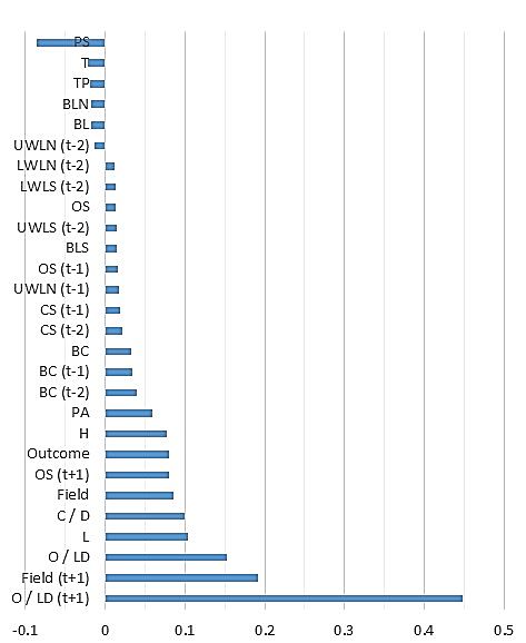
Appl. Sci. 2020, 10, 4484                                                                           2 of 18

and is highly suitable for use in conjunction with machine learning in predicting the price fluctuations
of financial commodities. As with the stock market, various analyses, such as fundamental, chip and
technical analyses, exist. For sports competitions, this study’s innovative proposal was to borrow the
technical analysis of the stock market and use candlesticks instead of indicators of sports performance
to make predictions.
      The purpose of this study is to present a methodology that combines the points scored and the
odds of the betting market to create a candlestick chart of a sports tournament. The study also aims to
extract the characteristics of machine learning modelling to predict match outcomes. To explore the
feasibility of our proposed classification and regression approaches based on machine learning, data
from a professional American football league (i.e., the National Football League, NFL) are used as
empirical evidence. Only a few studies with weak prediction accuracy are available as reference.
      The main contributions to the literature are as follows. First, we develop a consistent approach
that incorporates candlestick charts and machine learning for sports predictions without domain
knowledge in various sports. Second, we explore the impact of various candlestick features on the
predicted outcomes. Third, we compare the different approaches of machine learning models to reveal
which one can provide a more precise prediction. Fourth, we analyse in detail the differences in the
predictions between teams and between home and away teams.
      The rest of this paper is structured as follows. Section 2 contains an overview of related work.
Section 3 describes the dataset, proposed methodology and experimental design. Section 4 conducts a
performance analysis. Section 5 provides the concluding remarks and an outlook on our future work.

2. Related Work

2.1. Sports Forecasting and Machine Learning
      Based on previous research, methods of predicting the outcomes of matches can be divided
into two categories: namely, result-based and goal-based approaches. Result-based approaches aim
to predict the result class, whereas goal-based approaches aim to predict the goals scored by each
team in a certain match. In this context, predicting the winner and loser involves two approaches.
Result-based approaches are usually conducted using classification-based models, where the predicted
outcome is a categorical variable, such as win, loss or draw. Goal-based approaches are achieved
using regression-based models, where the predicted outcome is a numerical variable of a score or a
difference in score from that of the opponent, and the score is used to ascertain win, loss or draw. Other
approaches can be used to predict the outcome of a match, such as using the probability distributions
model to estimate win probability [1,2] or rating teams based on past performance and then predicting
based on rankings [3–5].
      Regardless of whether the model is classification–based or regression-based, the data used to
construct the model are mostly performance indicators, which are usually retrieved and calculated
from the offensive and defensive records of each team or each player. These performance indicators
produced on a statistical basis have been explored in many studies in various sports [6,7], and are often
used to predict the outcome of the game [8–10] and obtain explainable results.
      In addition to using performance indicators, situation variables, also known as conditional factors,
have been considered in many studies. Situational variables, such as match location, who scores first and
the quality of the opponent, can potentially affect the structure of a match and eventually the outcome
of the match; evidence has been presented to support the idea that situational variables are worth
including when analysing performance from a behavioural perspective [11,12]. Moreover, a play’s
position in the field is commonly considered in basketball [13,14] and football studies [9]. Additionally,
in international competitions among different national teams, the gross domestic production per capita,
population size and other relevant factors for each country have been considered [15,16].
      Sarmento et al. [17] systematically reviewed the variables commonly used in many football match
analysis studies and recommended the adoption of methodologies that include the general description
Appl. Sci. 2020, 10, 4484 3 of 18
of technical, tactical, physical performance, situational, continuous and sequential aspects of the game
to make the science of match analysis easy to apply in the field. Studies have considered many variables
to increase the complexity of the model. For example, Carpita et al. [9] used 33 player-related variables,
seven player performance indicators and the position of a player or a role. The explosion of a large
amount of input data accompanied by many variables has caused the traditional approach based
on the statistical model to have many dimensions. Thus, many studies have instead used machine
learning to process a large amount of data to construct black-box prediction models.
Utilising machine learning for predictive analysis has been studied in various sports
tournaments [18], such as basketball [19–21], baseball [22], cricket [23], ice hockey [24] and
football [25,26]. Many kinds of machine learning methods, such as artificial neural networks (ANNs),
support vector machines (SVMs), random subspace (RS), random forests (RFs) and hybrid modelling
approaches combining multiple methods, have been developed and used for comparison in match
result prediction.
2.2. Candlestick Charts and Machine Learning
Candlestick charting can be traced back to the Japanese rice trades and financial instruments
from centuries ago. It is a method for visualising data in different ways to predict recent stock price
fluctuations and provide insights into market psychology. Japanese candlestick theory has become
one of the most widely used technical analysis techniques for making investment decisions based on
empirical finances. Future trends in financial time series are considered to be predictable by identifying
specific candlestick patterns.
Some scholars have proposed ways to describe these known patterns with ordered fuzzy
numbers [27] or formal specifications [28] to provide recognition using machine learning. Some
scholars have characterised financial time series with candlestick charts and then used ANN, fuzzy
logic, genetic algorithms, decision trees and various hybrid approaches to provide predictions about
the market trend for investment decision use [29,30]. Given that candlestick charts incorporating
machine learning have been beneficial in the application of finance, some studies in other fields have
initiated applying them as a tool for analysis and prediction. They have been applied in studies on
predicting teens’ stress level change on a micro-blog platform [31] and in sports metrics [32] to forecast
game outcomes.
However, the application of candlestick charts in other fields is slightly beyond the applicability
of the original financial time series. They need to be adjusted and modified to accommodate specific
characteristics of the field. Whether candlestick charts exhibit certain patterns and corresponding
behaviours as in the financial field and whether they are equally suitable for pattern recognition using
machine learning to provide predictions are research areas to be examined.
2.3. Sports Forecasting in Betting Market
Betting on the sports market can be done in different ways. Regarding NFL games, Las Vegas
sports bookmakers provide two bets, namely, the point spread (side bet) between each pair of teams
and the total number of points scored by each pair of teams (over/under bet). Oddsmakers set the
numbers (lines) for these two bets by creating a margin between the two teams. The point spread (or
betting line) can be thought of as the betting market’s estimate of the difference between the points
scored by each team. If a gambler bets on the favourite, he or she wins the bet if the favourite wins by
more than the point spread. If a gambler bets on the underdog, he or she wins the bet if the underdog
either wins or loses by less than the point spread.
The betting market has many similar characteristics to financial markets [33]. Sports bookmakers
try to set their lines to ensure that an equal amount of money is bet on either side of the line. However,
if new information is received that changes the outlook of the match or if bettors tend to favour one
side of the line, then odds makers may change the line in the time leading up to the match to regain
the desired balance of bets. In terms of the phenomenon of commodity prices in the financial marketAppl. Sci. 2020, 10, 4484 4 of 18
reflected in the efficient market hypothesis, the same phenomenon can be seen in the odds of the
betting market. Balancing the bets on either side of the line is not always possible. Thus, the research
issue is whether any predictable pattern in the betting lines exists over the preceding week [34].
Bookmakers’ odds are implicit representations of all kinds of information, including the past
performance of players and teams, a mix of instant and asynchronous messages and a wide variety
of components of sports fan psychology; current stock prices reflect all information rationally and
instantaneously to the market in three forms, namely, weak, semi-strong and strong [35]. Moreover,
the random walk behaviour exhibited by stock price fluctuations makes the profit forecasting models
non-persistent for a long time, which can also be observed in the betting market. Although profit
forecasting models exist in the financial and betting markets during periods of market inefficiency [36],
extensive modelling innovations are required [37].
Many studies have recommended utilising betting market data released by bookmakers in
predictive models [38–40]. The results demonstrate that betting odds and margins have a rather high
predictive accuracy, which is justified because bookmakers cannot survive on inefficient odds and
margins. Thus, bookmakers’ predictions implied from the odds have often been used as a comparison
group in studies on match outcome prediction. Consequently, we suggest that betting markets should
also be relevant to the principles of stock market technical analysis. The historical data of the betting
market can be manipulated to draw candlestick charts to identify the features of the matches and used
for machine learning modelling to develop predictive models.
2.4. Analysis and Prediction of American Football
American football, such as NFL games, operates with a highly complex scoring system, making it
highly demanding to model the points scored using standard modelling approaches. NFL players can
score in five ways: an unconverted touchdown (six points), a touchdown with a one-point conversion
(seven points), a touchdown with a two-point conversion (eight points), a safety (two points) or a field
goal (three points). Other sports, such as football, baseball and basketball, follow relatively simple
rules for giving scores under limited conditions. Consequently, American football predictions are
highly challenging, regardless of whether traditional statistical models, modern machine learning
models or even bookmakers’ predictions are used, with lower accuracy than in other sports. However,
this challenge reveals opportunities for improvement in prediction models, leading to many studies
being devoted to it.
Song et al. [41] compared the prediction of the outcomes of NFL games by experts, statistical
models and opening betting lines on two NFL seasons. The findings showed that the distinctions
between experts and statistical systems in predicting the accuracy of contest winners were not
statistically significant and that betting lines performed better than the other two. David et al. [42]
analysed the ability of a neural network model to predict the outcome of NFL games. This model only
adopted readily available statistics, such as rushing yards, passing yards, fumbles lost and scoring,
and proposed the inclusion of differences in statistics between teams for comparison. Baker and
McHale [43] presented a point process model for forecasting end-of-match exact scores in NFL games.
Historical tournament information, including the teams’ scores, the field of play, records for each
game, various game statistics and data given by bookmakers, such as the margin (point spread) and
the over/under for each game, was obtained for the study. With a set of simple covariates based
on past match statistics, the model performed as well as bookmakers in predicting match outcomes
and exact scores. Pelechrinis and Papalexakis [44] collected play-by-play data from the past seven
seasons of the NFL and built a descriptive model for the probability of the home team winning a
game. A football prediction matchup engine was provided by combining this descriptive model with a
statistical bootstrap module. It achieved an overall accuracy of 63.4%, which outperformed the baseline
prediction based on win-loss standings every season. Schumaker et al. [45] examined the application
of techniques from technical charting used in stock price analysis to sentiment gathered from social
media for NFL game outcome prediction. The sentiment polarity was analysed as a time-series signal,Appl. Sci. 2020, 10, 4484 5 of 18
examining the position and magnitude of signal change between two temporal windows. The 50- and
200-day moving averages, which are popular techniques to analyse price movements in stock technical
charts, can be adopted to find patterns, such as golden and death crosses.
These NFL outcome prediction studies have employed different variables and methods. The
experiments within them were designed and measured in different ways. They used different datasets
to ensure that the criteria for accuracy were calculated differently and were not easy to compare.
However, most studies have compared their models with betting market predictions; some models
were better, and some were worse. Therefore, we suggest the use of interdisciplinary predictive models
that combine stock market technical analysis, betting market behaviour, sports prediction and machine
learning in data science. They have the potential to improve on previous approaches and lead to a new
research direction.
3. Methodology
3.1. Data Transformation into Candlestick
Candlestick charts used for sports outcome analysis are plotted based on the odds of the sports
betting market and the relative actual match outcome. Each candlestick represents a game. The line on
winning/losing margin between the team and its opponent (denoted as LD), the line on the total points
scored by both teams (denoted as LT), the actual margin (denoted as D) and the actual total points
scored (denoted as T) are gathered as the raw data for each game to plot the candlestick.
In general, a candlestick in the stock market is defined by the open-high-low-close (OHLC) price,
as shown in Figure 1a. In the sports betting market, we refer to Malios’s method [32] and take LD as
“open” and D as “close”. The gambling shock reflecting the gap between expectation and reality is
defined as the difference between a game outcome and its corresponding line. The difference between
“open” and “close” is treated as the gambling shock related to the line on the winning/losing margin
between the team and its opponent, denoted as GSD. GSD is similar to the price spread in the stock
market and forms the candlestick’s body length. The difference between LT and T is treated as the
gambling shock related to the line on the total points scored by both teams, denoted as GST. GST is
similar to the intraday price fluctuation degree in the stock market and forms the candlestick’s wick
length. If GST > 0, the wick extends above the body. If GST < 0, the wick extends below the body. If
GST = 0, no wick exists. In general, the wick is called the shadow, and the lower wick is called the tail.
The candlestick’s body colour is dependent on the relationship of D and LD. If D > LD, the body colour
is white, and the body’s maximum and minimum values are defined by D and LD. If LD > D, the body
colour is black, and the body’s maximum and minimum values are defined by LD and D. Figure 1b
illustrates the use of the candlestick chart in this study. The notations and definitions are as follows:
D: Team winning/losing margin (i.e., the difference in points scored between the team and its opponent)
LD: Line (or spread) on the winning/losing margin between the team and its opponent; the side line in
the betting market
T: Total points scored by both teams
LT: Line on the total points scored by both teams; the over/under (O/U) line in the betting market
GSD = D − LD (1)
GST = T − LT (2)
In this study, we redefine D by calculating the points scored by the opponent team minus the
points scored by the favourite team. The opposite value differs according to the value proposed by
Mallios. However, by this modification, winning/losing based on the negative/positive value of D and
LD becomes consistent. For example, when LD is −5.5, the favourite team wins and may exceed the
opposing team’s score by 5.5 points. In other words, if the value of LD is negative, the favourite teamCandlestick charts used for sports outcome analysis are plotted based on the odds of the sports
betting market and the relative actual match outcome. Each candlestick represents a game. The line
on winning/losing margin between the team and its opponent (denoted as LD), the line on the total
points scored by both teams (denoted as LT), the actual margin (denoted as D) and the actual total
points scored (denoted as T) are gathered as the raw data for each game to plot the candlestick.
Appl. Sci. 2020, 10, 4484 6 of 18
In general, a candlestick in the stock market is defined by the open-high-low-close (OHLC) price,
as shown in Figure 1a. In the sports betting market, we refer to Malios’s method [32] and take LD as
“open”
wins; if and
it is D as “close”.
positive, The gambling
the favourite team shock
loses. reflecting
Using thisthe gap between
method expectation
would reflect and reality
the gambling shockis
defined as the difference
appropriately.
Appl. Sci. 2020, 10, xFinally,
FOR PEER
between
the a game
candlestick
REVIEW
outcome
chart definedandby itsOHLC
corresponding
and the line.
bodyThe difference
colour between
are formulated
6 of 18
“open” and
as follows: “close” is treated as the gambling shock related to the line on the winning/losing margin
between
D: Teamthe team and its opponent,
winning/losing margin (i.e.,denoted asOGSD.
= LDGSD
the difference is similar
in points to thebetween
scored price spread in theand
the team stockits
(3)
market
opponent) and forms the candlestick’s ( body length. The difference between LT and T is treated as the
gambling shock related MAX (total
the D, LD ) + GST (if GST > 0)
LD: Line (or spread) on to
thethe
H line on
=
winning/losing points
margin scored
between by
theboth
teamteams,
and itsdenoted
opponent;as GST. GSTline
the side is
(4)
similar to the intraday MAX ( D, LD ) ( if GST < 0 )
in the betting market price fluctuation degree in the stock market and forms the candlestick’s wick
length.
T: Total points>scored
If GST 0, the wick extends
teamsabove the
(D,body.
LD) If(ifGSTGST< 0, > the
0) wick extends below the body. If
(
by both MIN
GST = 0, no wick exists. In L =
general, the wick is called the shadow, and (5)
LT: Line on the total points scored by MIN both
(D,teams;
LD) −the GST (if GST <
over/under 0) the
(O/U) linelower
in thewick is called
betting marketthe
tail. The candlestick’s body colour is dependent on the relationship of D and LD. If D > LD, the body
C =DD LD (6)
colour is white, and the body’s maximum and GSD minimum values are defined by D and LD. If LD >(1) D,
Tand
LT D > LD)values are defined by LD and(2)
(
the body colour is black, and the body’s maximum GSTWhite (ifminimum D.
Body color = (7)
Figure 1b illustrates the use of the candlestick chart Blackin(this > DThe
if LDstudy. ) notations and definitions are
In this study, we redefine D by calculating the points scored by the opponent team minus the
as follows:
points scored by the favourite team. The opposite value differs according to the value proposed by
Mallios. However, by this modification, winning/losing based on the negative/positive value of D
and LD becomes consistent. For example, when LD is −5.5, the favourite team wins and may exceed
the opposing team’s score by 5.5 points. In other words, if the value of LD is negative, the favourite
team wins; if it is positive, the favourite team loses. Using this method would reflect the gambling
shock appropriately. Finally, the candlestick chart defined by OHLC and the body colour are
formulated as follows:
O LD (3)
.
MAX(D, LD) GST (if GST 0)
H (4)
(a) MAX(D, LD) (if GST 0) (b)
Figure MIN(D,
data; LD) (if GSTdata. 0) The difference between “open” and
Figure 1.
1. Candlestick.
Candlestick. (a)
(a)Stock
Stockmarket (b) Sports
L data; (b) Sports data. The difference between “open” and (5)
market
“close” is treated as the gambling shock MIN(D,
related LD)
to -
theGST
“close” is treated as the gambling shock related to the line on line(ifonGST
thewinning/losing
the 0)
winning/losing marginmargin between
betweenthe the
team
teamand
andits itsopponent,
opponent,denoted
denotedasasGSD;
GSD;TheThedifference
difference between
between LT
LT (the
(the line
line on
on the
the total
totalpoints
points scored
scored
CD (6)
by
by both
both teams) and TT (the
teams) and (theactual
actualtotal
totalpoints
pointsscored)
scored)is is treated
treated as as
thethe gambling
gambling shock
shock related
related to the
to the line
line on total
on the the total points
points scored
scored by both
by both teams,
teams, Whiteas(ifGST.
denoted D LD)
Body denoted
color as GST.
(7)
Black (if LD D)
Seattle’s candlestick chart during the 2012–2013 and 2013–2014 seasons, including the pre-season,
Seattle’s candlestick chart during the 2012–2013 and 2013–2014 seasons, including the pre-
regular season, and post-season, is plotted in Figure 2 as an example.
season, regular season, and post-season, is plotted in Figure 2 as an example.
Figure 2.
Figure 2. Seattle’s
Seattle’s candlestick
candlestick chart
chart in
in 2012/2013 and 2013/2014.
2012/2013 and 2013/2014.
Some differences can observed between the candlestick charts for sports betting and stock prices.
First, the value of the stock price must be positive to ensure that the corresponding candlesticks
remain positive. However, the outcome of a game is either losing or winning. Thus, the
corresponding candlesticks can be positive or negative. Second, the typology of a stock candlestick is
diversification, but the appearance of a sports candlestick is limited. Sports candlesticks lack the typeAppl. Sci. 2020, 10, 4484 7 of 18
Some differences can observed between the candlestick charts for sports betting and stock prices.
First, the value of the stock price must be positive to ensure that the corresponding candlesticks remain
positive. However, the outcome of a game is either losing or winning. Thus, the corresponding
candlesticks can be positive or negative. Second, the typology of a stock candlestick is diversification,
but the appearance of a sports candlestick is limited. Sports candlesticks lack the type with the upper
and lower wick. Third, for stock candlesticks, the colour of a candlestick is consistent with the price
difference at opening and closing, and the stock price is up or down. However, the colour of the sports
candlestick is derived from the opening and closing differences but does not necessarily represent
winning or losing. Although the information covered by the sports candlestick chart is not as much as
that of the stock candlestick chart, the volatility of betting odds and the relationship of the time series
can also be graphically presented to provide another perspective and reference for analysts.
3.2. Feature Engineering and Selection
Regarding the fluctuations and predictions in stock prices in the financial market, we can make a
candlestick chart for sports, which reflects the time series of fluctuations in betting odds and actual
scores, and predict the results of sports games. How to describe the changes in these fluctuations and
extract the relevant characteristics is an issue to be investigated by this study.
We refer to some stock technique analysis concepts and use the following types of indicators as
characteristics of candlesticks. (a) OHLC: the OHLC sequence and its colour make up the candlestick
chart. (b) Length: the mean size of the candlestick’s body and wick includes the length of the body and
upper and lower wick. (c) Length style: the categories of length are very short, short, zero, long and
very long. (d) Relation style: the categories based on the relationship compared with the previous
candlestick are low, equal low, equal, equal high and high. This style is applied to describe the related
position of the open and close of the candlestick, referred to as the open style and close style. (e) Time
series: a series of variables indexed in time order. A variable denoted by V and the time series at data
points t − 2, t − 1 and t are expressed as V (t − 2), V (t − 1) and V (t), respectively.
When dealing with the length values of the body and wick, the maximum value of the margin
and the total score of the game can be found in previous game records, and the minimum value is zero.
Thus, we make the numerical scale of length consistent by min-max normalising to between 0 and 1
and then converting the length to a categorical variable, referred to as length style, depending on the
degree. The original value of the length, the normalised value of the length and the length style are
selected as features. However, special instances of zero length occur in many cases, such as a zero
upper wick and a zero lower wick, which cause the issue of imbalanced data in machine learning. To
address this issue, we specifically treat “zero” as a separate category of length style.
In this study, the length and relationship between adjacent candlesticks can be transformed into
categorical variables to become length, open and close styles, mainly considering the expression of the
candlestick pattern. The pattern of candlesticks can be expressed in several ways. Some studies have
used the exact threshold value to express the relationship with the previous candle as a percentage [28].
Some studies have expressed it in the form of fuzzy variables for fuzzy inference [29,46]. Given that
the pattern of the sports candlestick chart is unknown, it cannot be recognised by fuzzy inference.
However, we can still use fuzzy linguistic variables to characterise the features of the candlestick chart
appropriately, converting the numerical values into categories by setting the membership function.
Figure 3 illustrates the membership function of the linguistic variables for length style, which represents
the degree of the candlestick’s body or wick length. The x-axis in the figure indicates the length of the
body or wick on a normalised scale from 0 to 1. The categories of very long and very short on both
sides of the figure are defined by the linear membership function, and the categories of short and long
in the centre of the figure are defined by the triangle function.Appl. Sci. 2020, 10, 4484 8 of 18
Appl. Sci.
Appl. Sci. 2020,
2020, 10,
10, xx FOR
FOR PEER
PEER REVIEW
REVIEW 88 of
of 18
18
Figure3.3.
Figure
Figure 3.Membership
Membershipfunction
Membership functionof
function ofthe
of thelinguistic
the linguisticvariables
linguistic variablesfor
variables forlength
for lengthstyle.
length style.
style.
Thecandlestick
The
The candlestickpatterns
candlestick patternsalso
patterns alsoinclude
also includethe
include thecharacteristics
the characteristicsof
characteristics oftrends.
of trends.The
trends. Theconsequent
The consequenttrend
consequent trendof
trend ofthe
of the
the
candlestick
candlestick is is measured
measured by by
the the relationship
relationship between between
two two
adjacent adjacent
candlestick is measured by the relationship between two adjacent candlesticks. Comparing the candlesticks.
candlesticks. Comparing Comparing
the currentthe
current candlestick
candlestick
current candlestick with the
with the previous
with the previous
previous
one, one, the
the relative
one, the relativeofposition
position
relative position
the openof ofand
theclose,
the openreferred
open and close,
and close, referred
to as to as
open style
referred to as
open
and style
close and
style, close
is used style,
to is used
indicate to
the indicate
trend. the
Five trend.
linguisticFive linguistic
variables, variables,
namely,
open style and close style, is used to indicate the trend. Five linguistic variables, namely, low, equal low,namely,
equal low,
low, equal
equal,
low, equal,
equal
low, equal,and
high, equal
high,
equal high, and high,
are and
high, high,
defined are defined
to are defined
represent toopen
theto represent
and close
represent thestyle.
the open Figure
open and close
and close style.the
4 shows
style. Figure 44 shows
membership
Figure shows
the membership
membership
function
the function variables.
of these linguistic
function of these
of these linguistic
linguistic
The previous variables. The previous
candlestick
variables. The previous
is plotted candlestick
at the bottom
candlestick is plotted
is plotted at the
of the figure
at the
bottom
for of
comparison. the figure
The for
locationscomparison.
of the five The locations
linguistic of
variables the five
are
bottom of the figure for comparison. The locations of the five linguistic variables are plotted linguistic
plotted variables
according to the are plotted
previous
according to
candlestick
according to shown
as the previous
the previous candlestick
in the figure. as shown
The position
candlestick as shown in the
the figure.
of open/close
in figure.
for theThecurrent
The position of open/close
open/close
candlestick
position of for the
is located
for the
by
current
its
current candlestick
numerical value on
candlestick is located
is located
the x-axis,by its
by its
and numerical
the relation
numerical value
value on the
style
on thedetermined
is x-axis, and
x-axis, andaccording
the relation
the relation style
tostyle is determined
determined
the y-axis,
is which
according
gives the to the
possible y-axis,
value which
of the gives
membership the possible
function.value of
according to the y-axis, which gives the possible value of the membership function. the membership function.
Figure4.4.
Figure
Figure 4.Membership
Membershipfunction
Membership functionof
function ofthe
of thelinguistic
the linguisticvariables
linguistic variablesfor
variables foropen
for openand
open andclose
and closestyles.
close styles.
styles.
ToTocapture
To capturethe
capture thefeatures
the featuresofof
features ofcontinuous
continuoustime
continuous timevariation
time variationin
variation inthe
in thecandlestick
the candlestickchart,
candlestick chart,we
chart, wetreated
we treatedspecific
treated specific
specific
features
features as as
time time
series series
and and
considered considered
their data their
points data
in points
antecedent
features as time series and considered their data points in antecedent and posterior time in antecedent
and posterior and
time posterior
simultaneously time
assimultaneously
input variablesas
simultaneously as input
forinput variablesmodel.
the predictive
variables for the
for theThe predictive
candlestick
predictive model.
chartThe
model. The
of thecandlestick
stock market’s
candlestick chartdaily
chart of the
of the stock
trading
stock
market’s
data shows daily
the trading
two- and data
three-dayshows the
trading two- and
patterns three-day
presented by
market’s daily trading data shows the two- and three-day trading patterns presented by two andtrading
two andpatterns
three presented
successive by two
candlesticks,and
three successive
respectively. For candlesticks,
example, the respectively.
well-known engulfingFor example,
pattern is the
presented
three successive candlesticks, respectively. For example, the well-known engulfing pattern is well-known
by two engulfing
successive pattern
candlesticks, is
presented
which suggest
presented by atwo
by two successive
potential candlesticks,
trend candlesticks,
successive reversal. Thewhich which suggest aahas
first candlestick
suggest potential trend
a smalltrend
potential reversal.
body reversal.
that The first
is completely
The first
candlestick
engulfed by has
the a small
second body
candlestick.that is
It completely
is referred to engulfed
as a bullishby the
engulfing
candlestick has a small body that is completely engulfed by the second candlestick. It is referred second candlestick.
pattern when itIt is referred
appears at theto
to
as
end a bullish
as aofbullish engulfing
a downtrend
engulfing pattern
and pattern
a bearishwhenwhen
engulfingit appears at
patternatwhen
it appears the end
the end of
it appears a downtrend and
after an uptrend.
of a downtrend a bearish engulfing
Anotherengulfing
and a bearish example
pattern
ispattern when
the well-known it appears
evening after an
star, uptrend.
which is aAnother
bearish example
reversal is the
pattern
when it appears after an uptrend. Another example is the well-known evening star, which well-known
presented evening
by three star, which is
successive is
a bearish
candlesticks. reversal
The pattern
first presented
candlestick by
continues three successive
the uptrend. candlesticks.
The second
a bearish reversal pattern presented by three successive candlesticks. The first candlestick continues The first
candlestick candlestick
gaps up continues
and has a
the uptrend.
narrow
the uptrend.
body. The Thethird
The second
second candlestick
candlestick
candlestick closes gaps
gaps belowup and
up and has aa narrow
the midpoint
has narrow
of thebody.body. The third
third candlestick
first candlestick.
The candlestick closes
As a result, closes
three
below
consecutivethe midpoint
candlesticks, of the
V first
(t − candlestick.
2), V (t − 1) As
and Va result,
(t), can three
be usedconsecutive
below the midpoint of the first candlestick. As a result, three consecutive candlesticks, V (t − 2), Vas variablescandlesticks,
to predict V
the (t − 2),
outcome V (t(t
of− 1)
the and
nextV (t),
game can at be
t + used
1. as variables to predict the outcome
− 1) and V (t), can be used as variables to predict the outcome of the next game at t + 1. of the next game at t + 1.
In conjunction
In conjunction with with thethe above
above features
features of of the
the candlestick,
candlestick, the the field
field of
of the
the match
match in in the
the situation
situation
variable is adopted as a feature because it potentially affects
variable is adopted as a feature because it potentially affects the outcome of a match, such as the outcome of a match, such as home
homeAppl. Sci. 2020, 10, 4484 9 of 18
In conjunction with the above features of the candlestick, the field of the match in the situation
variable is adopted as a feature because it potentially affects the outcome of a match, such as home
advantage [47–49]. Moreover, the pre-game odds are considered as an important variable. Given
that the pre-game odds have already implied the predictions in bookmakers’ betting on the outcome
of the match, forecasting the outcome based on the odds and their volatility trend is an innovation.
Finally, all of the features selected as variables for the prediction model in this study are summarised
in Table 1. A total of 46 features corresponding to two different output variables can be selected to
build the classification-based and regression-based models.
Table 1. Description of the features used in this study.
Notation Description Categories
PS Point score Game result
PA Point allow Game result
TP Total points scored Game result
Field Match field, such as home or away Situation variable
Outcome Outcome, such as win or lose Game result
O/LD “Open” of the candlestick (i.e., the line on the margin) OHLC/betting
H “High” of the candlestick OHLC
L “Low” of the candlestick OHLC
C/D “Close” of the candlestick (i.e., the margin) OHLC/game result
T Total points scored by both teams (i.e., O/U) Betting
LT Line on T (i.e., O/U line) Betting
GST Gambling shock on T Betting
BL Body length of the candlestick (i.e., GSD) Length
BLN (t) Normalised BL of the candlestick at t, t − 1 and t − 2 Length (series)
BLS (t) BL style of the candlestick at t, t − 1 and t − 2 Length style (series)
UWL Upper wick length of the candlestick Length
UWLN (t) Normalised UWL of the candlestick at t, t − 1 and t − 2 Length (series)
UWLS (t) UWL style of the candlestick at t, t − 1 and t − 2 Length style (series)
LWL Lower wick length of the candlestick Length
LWLN (t) Normalised LWL of the candlestick at t, t − 1 and t − 2 Length (series)
LWLS (t) LWL style of the candlestick at t, t − 1 and t − 2 Length style (series)
BC (t) Body colour of the candlestick at t, t − 1 and t − 2 OHLC (series)
OS (t) Open style of the candlestick at t, t − 1 and t − 2 Relation style (series)
CS (t) Close style of the candlestick at t, t − 1 and t − 2 Relation style (series)
Field (t + 1) Known match field of the next game Situation variable
O/LD (t + 1) Known O/LD of the next game Betting/OHLC
LT (t + 1) Known LT of the next game Betting
OS (t + 1) Known OS of the next candlestick Relation style
Outcome (t + 1) Unknown outcome of the next game Output variable
C/D (t + 1) Unknown winning/losing margin of the next game Output variable
Note: t, t − 1 and t − 2 of the candlestick are the current game, previous game, previous two games, respectively.
OHLC: open-high-low-close; O/U: over/under; LT: the line on the total points scored by both teams; OS: open style
of the candlestick.
3.3. Data Source and Processing
This study focuses on the NFL. Data for the past 32 years were obtained from covers.com using
web scraping technologies in 2018. Only the data from after 2006 can be found since the recent website
revision. The original data included the pre-season, regular season and post-season for each team from
the 1985–1986 to 2016–2017 seasons, a total of 18,944 games.
The NFL currently has 32 teams. Each team plays 3 games in a pre-season and 17 games in a
regular season. The winner competes in the post-season to win the Super Bowl. For each season, we
selected the data from week 3 of the regular season to organise into datasets and discard the pre-season,
week 1 and week 2 data. The pre-season game mainly lets players warm up. Players take turns in the
field and gradually adjust themselves to their best condition. A pre-season game is slightly differentAppl. Sci. 2020, 10, 4484 10 of 18
in terms of the main players on the field. Thus, pre-season data were not used. The pattern of the
candlestick chart has at least three consecutive candlesticks that show the trend change to predict the
next game. Therefore, the data from week 1 and week 2 were combined with those of week 3 in the
regular season and were used as the parameters of the prediction model to predict the next match in
week 4. The rest of the data were organised into the input and output fields of the prediction model
sequentially. Data from the previous three games were used as the input, and the predicted win or loss
as the output.
This study is different from others in that both home and away teams were considered, instead of
only taking one team. Home team and away teams participate in a game. Some studies have taken the
home team’s perspective [9,10,22] and ignored the away team. Therefore, two records appeared in our
dataset for each game, one for the home team, and the other for the away team. In these two records,
the D, LD and colour of candlesticks are opposite. Given that the model parameters considered the field
factors, the data are not redundant and should be viewed as different time series for the different teams.
After reviewing the data, we found that 20 games were tied and could not be determined. This
situation rarely happens in the NFL (i.e., in less than 1% of all data). Thus, we treated it as an outlier
and deleted it. We also found that the value of LD in 236 games was zero, which means that the betting
booker’s prediction of the win/lose margin was zero and that the outcome could not be determined.
Given that the prediction model was not affected, the data were still adopted, but using betting market
forecasting as the comparison group inevitably became inaccurate.
Following filtering, deleting, calculating and transforming, the original data were sorted by year
and team name. A total of 13261 instances were obtained for the experiment in this study. Finally, to
meet the needs of the experiment, all of the data from the 32 seasons were split into training and testing
sets based on the season. The first 31 seasons (from 1985–1986 to 2015–2016), with 12831 instances,
were used as the training set to establish the prediction model. The last season (2016–2017), with 430
instances, was used as the testing set for evaluating the prediction model.
The data were split by season and year instead of by the percentage of data records because the
composition of the players and the coach was consistent in the same team for the same year [25]. Using
the candlestick chart to discuss the differences and trend changes in the concession games for teams in
the same season is meaningful. Moreover, a large number of data (i.e., 31 seasons’ worth of data) were
used as the training set, instead of only using the previous 5 or 10 seasons or separating the teams as
independent units. The main reason was to investigate whether the pattern derived from the overall
large amount of data implies a general pattern and improves prediction accuracy.
3.4. Experiment Design and Performance Evaluation
To forecast the win/lose outcome, this study investigated two approaches, namely, the
classification-based and the regression-based models. The output of the classification-based model
is a binary variable representing win or loss. The output of the regression-based model is a numeric
variable representing the win/lose margin. The win/lose margin is converted to the win/lose outcome.
The negative margin means a win, and the positive margin means a loss.
We tested the applicability of candlestick charts by using several machine learning methods for
each of the classification-based and regression-based models and compared the performance of the
prediction results. The choice of machine learning methods was based on existing empirical and
theoretical studies. RF and RS are supervised ensemble learning algorithms that can be used for
classification and regression problems. Multi-boosting (MB) and the M5 prime model tree (M5P) are
boosting ensemble algorithms that attempt to create a strong classifier from many weak classifiers.
MB was applied as a classification-based model, and M5P was used a model tree algorithm for the
regression-based model. SVMs are supervised learning models with associated learning algorithms
that analyse data used for classification and regression analysis. Sequential minimal optimisation
(SMO) is an algorithm widely used for training SVMs. The SMO algorithm for the SVM classifier
was selected for the classification-based model. The SMO algorithm for SVM regression (SMOReg)Appl. Sci. 2020, 10, 4484 11 of 18
was selected for the regression-based model. A multilayer perceptron (MLP) is a supervised learning
algorithm that has a wide range of applications in classification and regression in many domains.
We performed the experiments using the Weka machine learning package [50] using the default
settings without parameter adjustments. For all algorithms, the batch size was set to 100, which is the
preferred number of instances to process if batch prediction is being performed. For RF, the size of
each bag is set to 100% of the training set size. For further details, see [51]. For RS, a reduced error
pruning tree is chosen as the base classifier. The size of each subspace is set to 50% of the number of
attributes. For more information, see [52]. For MB, a decision stump is chosen as the base classifier.
The approximate number of subcommittees is set to 3. The weight threshold for weight pruning is
set to 100. Please refer to [53] for more information. For M5P, the minimum number of instances to
allow at a leaf node is set to 4. For further details about this approach, see [54]. For SMO, the kernel
is set to use a polynomial kernel and to use the logistic regression model as the calibration method.
The complexity parameter C is set to 1. Reference [55] explained the concept of SVM and SMO. The
SMOReg is set to use the polynomial kernel, with the complexity parameter C set to 1. The SVM
learning algorithm for regression is set to use SMO, according to Shevade, Keerthi, et al. [56]. For MLP,
the number of hidden layers is set to a, which is defined by the number of (attribute + classes) /2, and
the weight update is set with 0.3 learning rate and 0.2 momentum.
To compare these machine learning approaches with baseline strategies, we set two comparison
groups as a benchmark, namely, betting and home. Betting refers to the bookmaker’s prediction, which
is derived from the betting odds. Taking the winning/losing margin of a certain team in the betting
market odds, a negative value implies winning and a positive value implies losing. Home is when the
home team is always predicted to win the game, reflecting the well-known home advantage.
The performance of the forecasting models based on different machine learning approaches was
assessed by the accuracy of the win/lose outcome. The precision, recall and F-measure corresponding to
the outcome were also computed. For the accuracy, precision, recall and F-measure, greater values are
effectively considered better. Moreover, the forecasting error for model comparison was measured by
root mean square error (RMSE) and mean absolute error (MAE), which have been widely used in many
studies. For the classification-based model, RMSE and MAE reflect the error of the estimated numerical
values within the model, not the error of classification. The estimated values can be converted into
predictions of win-loss outcomes given by the model itself. However, the regression-based model
directly output the numerical margin value with RMSE and MAE. Then, we transferred it to determine
the win/lose outcome. For RMSE and MAE values, generally the smaller the better, which means the
predicted responses are close to the true responses.
4. Experimental Results and Discussion
4.1. Feature Selection Results
This study explores whether odds, scores and the derived candlestick chart can be used to predict
the outcome of a match. Several relevant variables were listed as the characteristics representing
candlestick behaviour. We further carried out feature engineering to select the most influential factors
as the input value of the forecasting model and reduce the number of variables to lower complexity.
For the classification-based model, the importance of the features was evaluated by calculating the
Pearson correlation. The information gain (InfoGain) and information gain ratio (GainRatio), which
are entropy-based metrics commonly used in classification, were calculated for comparison. Among
the 46 features, based on the result of the Pearson correlation calculation, all correlation coefficients
were greater than zero, of which 26 were greater than 0.01. The calculation results for GainRatio and
InfoGain were similar for all 46 features, and 16 of them had a value of 0. We selected 26 features with
a Pearson correlation greater than 0.01, excluded those whose GainRatio and Infogain were zero, and
selected 19 features as input variables.Appl. Sci. 2020, 10, x FOR PEER REVIEW 12 of 18
GainRatio and InfoGain were similar for all 46 features, and 16 of them had a value of 0. We selected
26 features
Appl. Sci. 2020, with
10, 4484a Pearson correlation greater than 0.01, excluded those whose GainRatio12 and of 18
Infogain were zero, and selected 19 features as input variables.
For the regression-based model, only the Pearson correlation was used for feature selection. The
For theresults
calculation regression-based model, only
of all 46 features the Pearson
had positive correlation
or negative was used coefficients.
correlation for feature selection.
We tookThe 22
calculation results of all 46 features had positive or negative correlation coefficients.
features with correlation coefficients greater than 0.01 and six features with correlation coefficients We took 22 features
withthan
less correlation
−0.01. Acoefficients greater than
total of 28 features were0.01
usedand six features
as input with
variables forcorrelation
the model.coefficients less than
−0.01. A total of 28 features were used as input variables for the model.
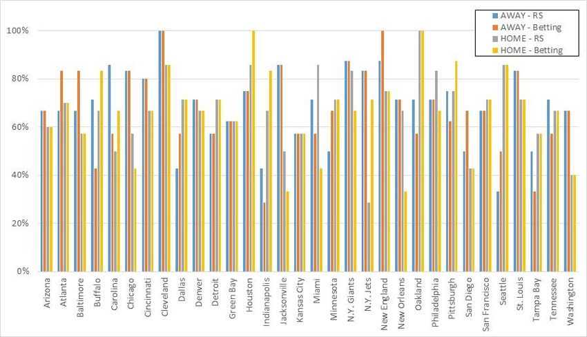
We present the results of feature selection and their correlation coefficients in Figure 5. The
figureWe present
shows that,theforresults of feature selectionmodel,
the classification-based and their
thecorrelation
OHLC andcoefficients in Figure
field are more 5. The
important figure
factors,
shows that,
whereas bodyforlength,
the classification-based
lower wick and model,
LT do notthe affect
OHLCthe andclassification
field are more important
result and are factors, whereas
not included.
body length, lower wick and LT do not affect the classification result and are not
For the regression-based model, OHLC and field affect the results, and almost all the characteristics included. For the
regression-based
of the candlestickmodel, OHLC and
are included. field affect
Finally, whetherthe results, and almost
classification all the characteristics
or regression, the top six of the
most
candlestickfactors
important are included.
influencing Finally, whether
prediction are classification
the same, andorthe regression,
top three the
are top six most
LD(t+1), important
Field(t+1) and
factors
LD order. prediction are the same, and the top three are LD(t + 1), Field(t + 1) and LD in
influencing
in that
that order.
(a) (b)
Figure
Figure 5.5.Correlation coefficients
Correlation of selected
coefficients features.
of selected (a) Classification-based
features. models, (b)models,
(a) Classification-based regression-
(b)
based models.
regression-based models.
4.2. Comparison
4.2. Comparison of
of Different
Different Approaches
Approaches
In this
In this study,
study, we adopted the data on points scoredscored and betting odds
odds to
to plot
plot the
the candlestick
candlestick and
and
used them
used them asas the
the input
input data
data to
to forecast
forecast the
the outcome
outcome ofof the
the next
next game.
game. To
To explore
explore whether
whether this
this can
can be
be
applied to the models constructed by different machine learning algorithms and achieve
applied to the models constructed by different machine learning algorithms and achieve satisfactorysatisfactory
accuracy, we
accuracy, weconstructed
constructedclassification-based and and
classification-based regression-based modelsmodels
regression-based using a using
different
a approach.
different
The prediction
approach. results are results
The prediction shown arein Tables
shown2 in
and 3. 2 and 3.
Tables
Table 2.
Table Performance of
2. Performance of the
the classification-based
classification-based models.
RFRF RSRS MB
MB SMO
SMO MLP
MLP
Accuracy
Accuracy 0.6279
0.6279 0.6512
0.6512 0.6767
0.6767 0.6465
0.6465 0.6186
0.6186
Correct
Correct instances
instances 270270 280280 291291 278278 266266
MAE
MAE 0.4503
0.4503 0.4483
0.4483 0.3408
0.3408 0.3535
0.3535 0.4191
0.4191
RMSE 0.4820 0.4687 0.5287 0.5945 0.4899
RMSE 0.4820 0.4687 0.5287 0.5945 0.4899
Note: RF: random forests; RS: random subspace; MB: Multi-boosting, SMO: Sequential minimal optimisation, MLP:
Note: RF: random forests; RS: random subspace; MB: Multi-boosting, SMO: Sequential minimal
multilayer perceptron, MAE: mean absolute error, RMSE: root mean square error.
optimisation, MLP: multilayer perceptron, MAE: mean absolute error, RMSE: root mean square error.Appl. Sci. 2020, 10, 4484 13 of 18
Table 3. Performance of the regression-based models.
RF RS M5P SMOReg MLP
Accuracy 0.6442 0.6837 0.6814 0.6744 0.5326
Correct instances 277 294 293 290 229
MAE 9.5604 9.4005 9.0534 9.1117 13.872
RMSE 12.1827 11.9499 11.6326 11.6865 17.6083
Note: M5P: M5 prime model tree, SMOReg: The SMO algorithm for SVM regression.
In the comparison group, of the 430 testing cases, 290 were correct for betting and 254 for home.
We used the comparison group as a comparison benchmark for each model. In the classification
model, only MB, with 291 cases correct, was better than the comparison group. The remaining models,
regardless of the algorithm used, were not as accurate as betting in the comparison group. In the
regression model, RS, M5P and SMOReg with 294, 293 and 290 test cases correct, respectively, were
better than the comparison group. Although the accuracy rate of these models was higher than that of
the comparison group, only a slight improvement of zero to four cases can be observed. Overall, the
regression model is more feasible for the prediction of the outcome than the classification model.
However, among these models, the model with the highest accuracy rate does not necessarily
have the smallest error measurement. For example, RS in the classification-based model performed
best when measured by RMSE, but its accuracy rate was second best. In the regression-based models,
although the accuracy of RS was the best, the error measurement in MAE and RMSE was inferior
to that of M5P and SMOReg. RS, RF and MLP can be used for constructing classification-based and
regression-based models. Only RS performs well in both types of models. However, RF and MLP did
not perform better than betting in the comparison group, which may be because we did not tune the
parameters of these algorithms and did not use the optimised parameter settings.
We further took the best model out of the classification-based and regression-based models and
examined the comparison group, as shown in Table 4. Examining all the data in the table to compare
the prediction model, we found that the RS of the regression-based model was the best among the
classification-based model, regression-based model and two comparison groups, and that its F-measure
was also the best. The worst was home in the comparison group, which reflects the home advantage
effect, but the accuracy was still at 59%, which is higher than the random neutral at 50%. We also found
that the classification model is almost the same as betting in the comparison group. The maximum
value in the table is 70.83%, which appears in the recall for the regression-based RS model. Therefore,
when RS predicts a win, it is 70.83% correct.
Table 4. Comparison of different approaches.
Classification Regression Comparison Group
MB RS Betting Home
Accuracy 0.6767 0.6837 0.6744 0.5907
Precision 0.6791 0.6770 0.6776 0.5926
Recall 0.6759 0.7083 0.6713 0.5926
F-measure 0.6775 0.6923 0.6744 0.5926
The kappa coefficient is a measure of inter-rater agreement involving binary forecasts, such
as win-lose [57]. We used the kappa coefficient for measuring the levels of agreement among ML
approaches against the comparison groups and actual outcome. Table 5 shows the results of the kappa
coefficient. In Table 5, it can be seen that the level of agreement reached the degree of almost perfect
(>0.81) among MB and RS against the betting. In addition, there was greater agreement in MB against
the betting than in RS.You can also read