Risk Assessment and Mapping of Hand, Foot, and Mouth Disease at the County Level in Mainland China Using Spatiotemporal Zero-Inflated Bayesian ...
←
→
Page content transcription
If your browser does not render page correctly, please read the page content below
International Journal of
           Environmental Research
           and Public Health

Article
Risk Assessment and Mapping of Hand, Foot, and
Mouth Disease at the County Level in Mainland
China Using Spatiotemporal Zero-Inflated Bayesian
Hierarchical Models
Chao Song 1,2 , Yaqian He 3 , Yanchen Bo 1, *             ID
                                                               , Jinfeng Wang 4 , Zhoupeng Ren 4   ID
                                                                                                        and
Huibin Yang 1
 1    State Key Laboratory of Remote Sensing Science, Institute of Remote Sensing Science and Engineering,
      Faculty of Geographical Science, Beijing Normal University, Beijing 100875, China; songc345@163.com (C.S.);
      yanghb@mail.bnu.edu.cn (H.Y.)
 2    School of Geoscience and Technology, Southwest Petroleum University, Sichuan 610500, China
 3    Department of Geology and Geography, West Virginia University, Morgantown, WV 26505, USA;
      heyaqian1987@gmail.com
 4    State Key Laboratory of Resources and Environmental Information System (LREIS),
      Institute of Geographic Sciences and Natural Resources Research, Chinese Academy of Sciences,
      Beijing 100101, China; wangjf@lreis.ac.cn (J.W.); renzp@Lreis.ac.cn (Z.R.)
 *    Correspondence: boyc@bnu.edu.cn; Tel.: +86-10-5880-2062

 Received: 16 June 2018; Accepted: 10 July 2018; Published: 12 July 2018

 Abstract: Hand, foot, and mouth disease (HFMD) is a worldwide infectious disease, prominent in
 China. China’s HFMD data are sparse with a large number of observed zeros across locations and
 over time. However, no previous studies have considered such a zero-inflated problem on HFMD’s
 spatiotemporal risk analysis and mapping, not to mention for the entire Mainland China at county
 level. Monthly county-level HFMD cases data combined with related climate and socioeconomic
 variables were collected. We developed four models, including spatiotemporal Poisson, negative
 binomial, zero-inflated Poisson (ZIP), and zero-inflated negative binomial (ZINB) models under the
 Bayesian hierarchical modeling framework to explore disease spatiotemporal patterns. The results
 showed that the spatiotemporal ZINB model performed best. Both climate and socioeconomic
 variables were identified as significant risk factors for increasing HFMD incidence. The relative risk
 (RR) of HFMD at the local scale showed nonlinear temporal trends and was considerably spatially
 clustered in Mainland China. The first complete county-level spatiotemporal relative risk maps
 of HFMD were generated by this study. The new findings provide great potential for national
 county-level HFMD prevention and control, and the improved spatiotemporal zero-inflated model
 offers new insights for epidemic data with the zero-inflated problem in environmental epidemiology
 and public health.

 Keywords: HFMD; spatiotemporal zero-inflated modeling; climate and socioeconomic factors;
 spatiotemporal mapping; Bayesian Hierarchical method

1. Introduction
     Hand, foot, and mouth disease (HFMD), mainly occurring in young children, is a worldwide
infectious disease caused by enterovirus and can lead to death [1]. The most obvious symptom
of HFMD is that patients have small herpes or ulcers in positions of hand, foot, and mouth on
the body. HFMD is mainly transmitted through air and close contact [1–3]. In China, HFMD is a
leading infectious disease and has been formally incorporated into the national monitoring system,

Int. J. Environ. Res. Public Health 2018, 15, 1476; doi:10.3390/ijerph15071476            www.mdpi.com/journal/ijerph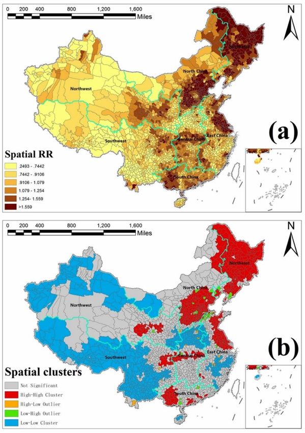
Int. J. Environ. Res. Public Health 2018, 15, 1476                                              2 of 16

since May 2008 [2]. From 2008 to 2013, China’s HFMD incidence rate increased remarkably from
37.6/100,000 persons to 139.6/100,000 persons [3]. HFMD has posed a serious threat to China’s
public health security. However, the spatiotemporal epidemics of HFMD across Mainland China are
still unclear.
      Previous studies have revealed that HFMD is strongly associated with climate environmental
factors including temperature [4,5], humidity [6,7], precipitation [8,9], wind speed [10,11], air
pressure [12], and sunshine [13]. Climate conditions not only impact the reproduction and transmission
of the viruses causing HFMD, but also change the physical activities of children [14], which together
promote the opportunity for viral contact among young children [15]. Socioeconomic factors may also
modify the climate effects on HFMD [16–18]. However, few studies concerned both socioeconomic
and climate factors for HFMD risk assessment and mapping, especially on the spatiotemporal
scales. In addition, previous HFMD studies in China mainly focused on small regions, such as
Guangdong [19], Shandong [20], Beijing [21], Shenzhen [10], and Sichuan [22]. Whereas, with regard
to Mainland China [16,17,23–25], no studies have established spatiotemporal final scale risk maps of
HFMD at the county level, not to mention accounting for both climatic and socioeconomic factors.
      Moreover, epidemiological data for disease mapping with excessive zeros is defined as a
zero-inflated (ZI) problem [26], because most diseases are on rare conditions. China’s HFMD
surveillance data suffered a serious ZI problem because they were collected at the county level,
the smallest national administrative division unit [16]. Ignoring the ZI problem in epidemiological
data could drop important disease characteristics, reduce disease relative risk (RR) mapping accuracy
and increase uncertainty [26]. Former studies have considered ZI effects for other diseases [27–30],
however, to our best knowledge, no studies have considered the ZI problem for HFMD risk assessment
and mapping.
      Zero-inflated models have been widely used for handling count data with excessive zeros [31,32],
among which zero-inflated Poisson (ZIP) and zero-inflated negative binomial (ZINB) are the two
most popular ones [33]. In addition, spatiotemporal models have gained popularity for disease risk
assessment and mapping in epidemiology [34,35]. Arab et al., have presented a review of an advanced
methodology combining spatiotemporal and zero-inflated models for spatial and spatiotemporal
epidemiological data with excessive zeros [26]. Recently, the spatiotemporal ZI models have drawn
much attention in environmental epidemiology and public health. For instance, Musenge et al. utilized
Bayesian spatiotemporal zero-inflated models for HIV/TB in South Africa [29]. Amek et al. applied a
zero-inflated binomial model for spatiotemporal modeling of sparse geostatistical malaria sporozoite
rate data in Kenya [28]; Musio et al. used Bayesian semi-parametric ZIP models with space-time
interactions for lymphoid leukemia incidence data in France [36]. Spatiotemporal models are preferably
specified within the Bayesian hierarchical modeling (BHM) framework because BHM can account for
ZI effect and similarities based on the neighborhoods among space and time flexibly [34,35] and has
been widely used in environmental epidemiology [37,38]. However, such spatiotemporal zero-inflated
models have not been utilized to solve the ZI problem for HFMD.
      To address the aforementioned shortcomings in current HFMD studies, we built spatiotemporal
ZIP and ZINB models under the BHM framework, accounting for both climatic and socioeconomic
covariates, using the monthly county-level HFMD cases data across the whole Mainland China in
2009. The objective of this paper is four-fold: (1) to test the effectiveness of ZI influence between
spatiotemporal ZI models and traditional models, (2) to identify environmental risk factors for HFMD
considering both climatic and socioeconomic aspects, (3) to fit the spatial clusters and nonlinear
temporal trend of HFMD relative risks, and (4) to estimate the complete spatiotemporal risk maps at
county-level in Mainland China.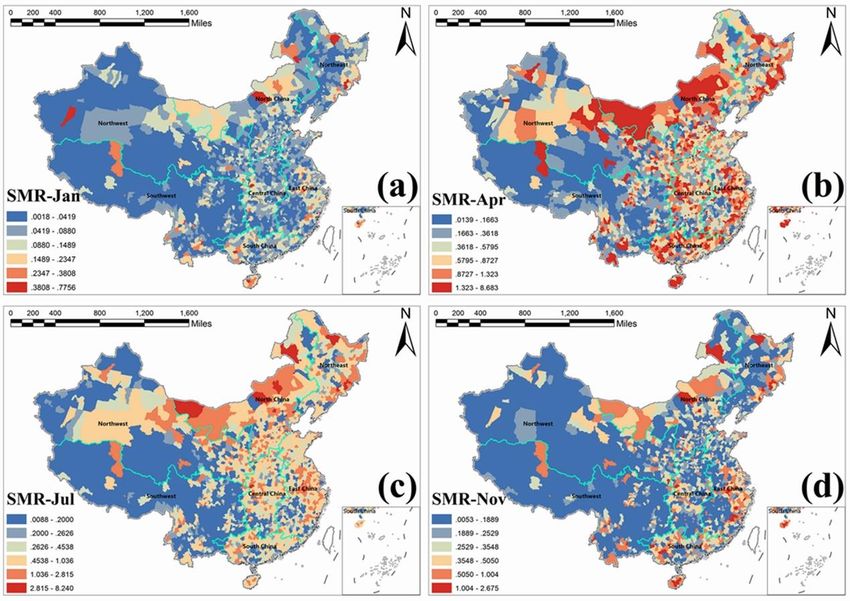
Int. J. Environ. Res. Public Health 2018, 15, 1476 3 of 16
Int. J. Environ. Res. Public Health 2018, 15, x 3 of 16
2. Materials
2. Materials and
and Methods
Methods
2.1. Data and Study Area
2.1. Area
For the
For the study
study area
area of
of Mainland
Mainland China,
China, we acquired
acquired county-level
county-level monthly
monthly data
data including
including HFMD
HFMD
cases, climate, and
cases, and socioeconomic
socioeconomicvariables
variablesfor forthe
theyear
year2009.
2009.A A total of of
total 2310 counties
2310 countieswere valid
were for
valid
analysis.
for analysis.
HFMD case
HFMD casedatadataininchildren
childrenagedagedbetween
between 0–90–9 years
years was was from
from thethe China
China Information
Information System
System for
for Disease
Disease Control
Control and Prevention
and Prevention (CISDCP).
(CISDCP). In the
In the year year
2009, 2009,
there there
were were
about about 1,166,000
1,166,000 HFMD cases HFMD
and
cases
the and the
HFMD HFMD rate
incidence incidence rate was 75.84/100,000
was 75.84/100,000 children
children across across China.
Mainland Mainland TheChina.
highest The highest
incidence
incidence
rate occurredrateinoccurred
April with in13.77/100,000
April with 13.77/100,000
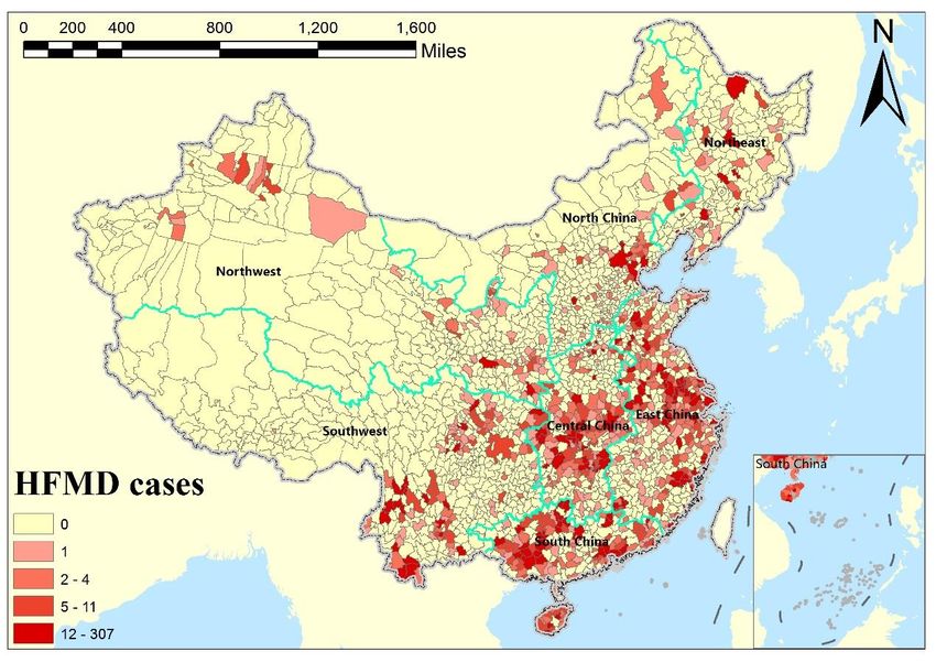
children. Figure children.
1 shows Figure 1 shows thedistribution
the geographical geographical of
distribution
reported HFMDof reported
cases inHFMD
Mainland cases in Mainland
China in January China
2009, inwhere
January 2009,number
a large where aof large
areasnumber
are withof
areas are
“zero” with “zero”
occurrences. occurrences.
China’s China’s HFMD
HFMD epidemic epidemic
data suffers datazero-inflation
a serious suffers a serious zero-inflation
problem, thus it is
problem, thus
necessary it is necessary
to consider to consider
the ZI effect the risk
in disease ZI effect in disease
assessment andrisk assessment and mapping.
mapping.
The monthly
The monthly climate data in this this study
study waswas based
based on on the
the raw
raw data
data collected
collected from
from 727
727 climate
climate
stations throughout
stations throughout ChinaChina from
from the
the China
China Climate
Climate Data
Data Sharing
Sharing Service
Service System
System [16].
[16]. Data of yearly
yearly
socioeconomic variables
socioeconomic variables were
were from
from the China County Statistical Yearbook, China Statistical Yearbook
for Regional
for Regional Economy,
Economy, and and China
China City
City Statistical
Statistical Yearbook
Yearbook [39].
[39]. We
We included
included aa total
total of
of six
six climatic
climatic
variables and
variables and fourteen
fourteen socioeconomic
socioeconomic variables
variables as as the
the potential
potential environmental
environmental riskrisk factors
factors for
for HFMD
HFMD
in this
in this study
study (Supplementary
(Supplementary File File S1,
S1, Table
TableS1).
S1).
Figure 1.
Figure 1. Geographical
Geographical distribution
distribution of reported hand, foot, and mouth disease (HFMD)
(HFMD) cases
cases in
in
Mainland China
Mainland China in
in January
January 2009.
2009.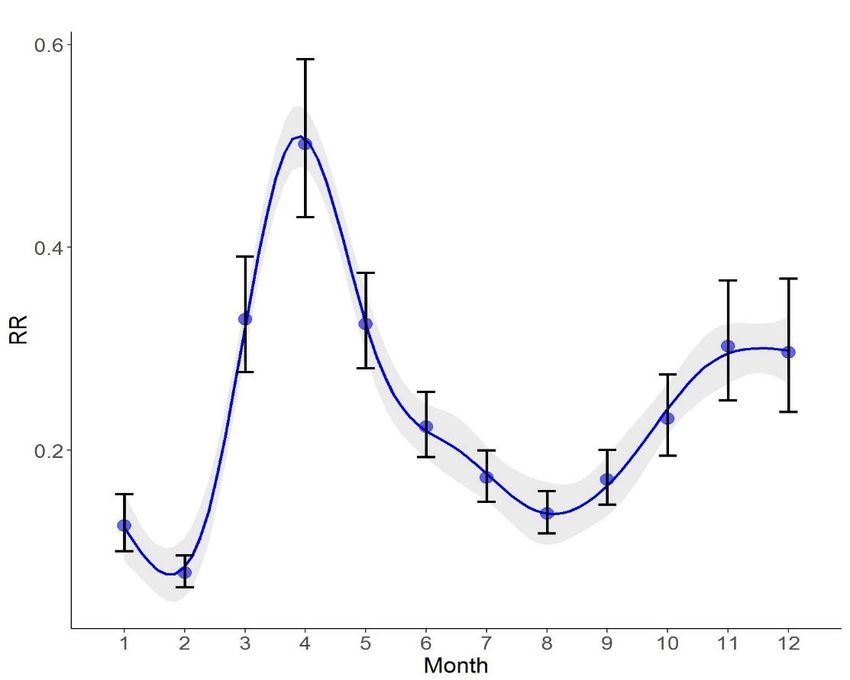
Int. J. Environ. Res. Public Health 2018, 15, 1476                                                        4 of 16

2.2. Statistical Models

2.2.1. Spatiotemporal Epidemic Models
      Within the study area, we denote the county-level areal units as i = 1,..., I (I = 2310) and the months
as t = 1,..., T (T = 12). In epidemiology, conditional to the relative risk λit , the rare disease cases Yit are
usually assumed to be Poisson-distributed. The likelihood function in spatiotemporal Poisson model
is expressed as follows [40]:
                                            Yit ∼ Poisson( Eit λit )                                         (1)

where Eit is the expected value for area i and time t. λit is the target estimated variable and is explained
as the standard morbidity ratio (SMR) [36]. Disease cases are usually rare or zero in areas with small
populations, which leads to extreme incidence values for direct disease mapping. The SMR map can
smooth the extreme outliers and give more intuitive information, and thus has been widely used for
disease risk mapping [41].
     With Poisson data assumption, the spatiotemporal model we applied in this study is decomposed
additively into components regarding climate and socioeconomic covariates, space, and time:
                                                            m                 n
                           ηit = log(λit ) = β 0 + ∑ β k Ck + ∑ α j SEj + µi + νi + γt + ϕt                  (2)
                                                             k                j

where ηit is the structured additive linear predictor; λit is estimated SMR of HFMD in space i and time
t; Ck is the k-th climatic environmental variables; SEj is the j-th socioeconomic environmental variables;
β 0 quantifies the intercept fixed effect; β k quantify climate fixed effects; α j quantify socioeconomic
fixed effects; and µi , νi , γt , ϕt represent main spatial and temporal random effects [34,35].
      Relative risk (RR) is widely used to measure the risk of disease exposure to a determinant in
epidemiology [42]. Risk indicator RR can be obtained directly using RR = e β . In epidemiology, an RR
value higher than one indicates that the exposure variable is a positively correlated risk factor, lower
than one means a negatively correlated risk factor, and equal to one means an unrelated factor.
      Regarding the spatial components including two spatial random effects: one assumes an
independent Gaussian exchangeable prior to model unstructured heterogeneity, which is νi ∼ N (0, δν2 ),
and the other one assumes an intrinsic conditional autoregressive (CAR) prior for the spatially
structured variability [43], which is as follows:

                                                                           1             σ2
                                                     µi | µ j 6 =i ∼ N (      ∑
                                                                           mi i ∼ j
                                                                                    µi ,
                                                                                         mi
                                                                                            )                (3)

where i ~j indicates that areas i and j are neighbors, mi is the number of areas that share boundaries
with the i-th area, and σ2 is the variance component. Spatial dependence in µi assumes the CAR prior
that extends the well-known Besag model [43] with a Gaussian distribution and implies that each µi is
conditional on the neighbor µ j with variance dependent on the number of neighboring counties mi of
county i.
     The CAR prior model assumes that the disease incidence risk in a spatial area is derived
from nearby geographical neighbors. That is, the closer the space distances, the more similar
disease incidence risk is in these spatial areas. This structured spatial character is called spatial
autocorrelation [44]. On the contrary, the Gaussian prior model for the unstructured spatial effect
represents the spatial heterogeneity, in which the spatial areas are independent of each other.
     Regarding the temporal components: the term φt is the unstructured time effect, which is specified
using an independent mean-zero normal prior to the unknown variance σφ2 ; the term γt represents the
structured time effect and is modeled dynamically through a neighboring structure. Here, the random
Int. J. Environ. Res. Public Health 2018, 15, 1476 5 of 16
walk (RW) dynamic model is used as a prior for the structured time effect [45], whose prior density π
is written as follows:
1 T
π (γt σγ2 ) ∝ exp(− 2 ∑ (γt − γt−1 )2 ) (4)
2σγ t=2
Similar to CAR, the RW prior model assumes that the disease incidence risk is influenced by
adjacent time points (temporal correlation). The temporal variation of disease risk is assumed to
be a smoothly varying curve, and when this structured temporal trend is nonlinear, the RW model
is more suitable. The independent prior model for the unstructured temporal effect represents the
temporal heterogeneity.
Similar to the RR calculation aforementioned, we could also obtain the local RRs for the structured
spatial and temporal random effects with RRi = eµi and RRt = eγt , respectively. The interpretation
of local RR is also similar. The higher the RR, the higher the risk. For instance, a spatially local RR
greater than one indicates that the spatial unit is a high-risk area, an RR value less than one indicates
that the spatial unit is a low-risk area, and an RR equal to one means that the risk of the areal unit is on
an average level.
In addition, except for the aforementioned Poisson distribution, the negative binomial distribution
is particular for delineating the distribution of positive integer count data. As HFMD cases are
positive integer data, the negative binomial distribution is also suitable. The likelihood function in a
spatiotemporal negative binomial model is written as follows:
Yit ∼ nBinomial ( Eit λit ) (5)
2.2.2. Zero-Inflated Models
A disproportionately large frequency of zeros in the aggregated epidemic data leads to a poor
performance of Poisson models for relative risk. To overcome this issue, the so-called zero-inflated
model is a promising method. A zero-inflated model is a mixture model with two components: one
arising from a parent distribution and the other corresponds to the excessive zeros that cannot be
accounted for by the distribution [32]. In this study, we introduced two commonly used zero-inflated
models to further develop the spatiotemporal model [26]. One is the zero-inflated Poisson (ZIP)
model [46], and the other one is the zero-inflated negative binomial (ZINB) model [33].
The ZIP model is described as follows [33,46]:
(
pit + (1 − pit ) f (0), yit = 0
P(Yit = yit ) = (6)
(1 − pit ) f (yit ), yit > 0,
λit yit
f (yit ) = exp(−λit ) (7)
yit !
where Yit is a count variable and λit > 0. p represents the probability of the existence of extra zeros.
When p is 0, the model is a Poisson distribution.
Compared with the ZIP model, the ZINB model [32,33] is more reliable to explain the large
dispersion structure of data. Similarly, we assume that f (yit ) following a negative Binomial
distribution, the ZINB model is described as follows:
(
pit + (1 − pit ) f (0), yit = 0
P(Yit = yit ) = (8)
(1 − pit ) f (yit ), yit > 0,
yit
Γ(yit + α) α α λit
f (yit ) = ( ) ( ) (9)
yit !Γ(α) α + λit α + λit
where α−1 is a dispersion parameter and p is the zero expansion parameter. When p is 0, the model is a
negative Binomial distribution.Int. J. Environ. Res. Public Health 2018, 15, 1476 6 of 16
2.2.3. Spatiotemporal Zero-Inflated Models
To evaluate the performance of incorporating ZI models in spatiotemporal modeling for our case,
we built four models for comparison. These four models had the same components as Equation (2),
including covariate information in the spatiotemporal process, but assuming different data distribution
models. Specifically, data distributions in the four models are as follows:
The traditional spatiotemporal Poisson model (herein referred to as model 1) is given by Equation (1);
The spatiotemporal negative Binomial model (herein referred to as model 2) is given by Equation (5).
The spatiotemporal ZIP model (herein referred to as model 3) is given as follows:
Yit ∼ ZIP( Eit λit ) (10)
The spatiotemporal ZINB model (herein referred to as model 4) is given as follows:
Yit ∼ ZI NB( Eit λit ) (11)
With the spatiotemporal ZI models, the SMR estimation can take into account ZI influence
and comprehensively incorporate the climate and socioeconomic environmental covariates, spatial
autocorrelation effect, and temporal nonlinear variations.
2.2.4. Covariates Selection
Before modeling, one important step is to select representative variables from a variety of potential
variables. Three criterion strategies were used for selecting the candidate climate and socioeconomic
variables in this study. Firstly, the variance inflation factor (VIF) for each candidate variable was
calculated to assess the multicollinearity [47]. The larger the VIF, the more severe the multicollinearity.
Normally, the variables selection considers VIF < 10 as the screening standard. Secondly, we used
the forward stepwise regression method to exclude the variables without statistical significance [16].
We set 0.05 and 0.1 as the threshold significance values. Finally, covariates were retained in the model
unless their removal resulted in the increase of deviance information criterion value by 30 units or
more [48].
2.3. Model Evaluation Methods
2.3.1. Deviance Information Criterion
The deviance information criterion (DIC) method is a well-known model criterion for comparing
Bayesian models’ fitness and complexity, defined as follows [49]:
DIC = D + PD (12)
where D is the mean of model posterior deviance and PD is the effective number of parameters.
A large D indicates a great error in the model. A large PD indicates a high complexity of the model.
The smaller the DIC and the PD , the better. Models with smaller DIC indicate a better trade-off
between complexity and fitness of the model.
2.3.2. Conditional Predictive Ordinate
The conditional predictive ordinate (CPO) is defined as a leave-one-out cross-validated predictive
density at a given observation and can be used to access predictive quality [50]. For continuous
distributions, it is defined as follows:
CPOit = p(yit∗ y f ) (13)Int. J. Environ. Res. Public Health 2018, 15, 1476 7 of 16
where yit∗ is the predicted value and y f is the sample of observations y, which is used to fit the model
and to estimate the posterior distribution of the parameters. In practice, the cross-validated logarithmic
score (LS) computed from CPO is widely used to evaluate the predictive quality for Bayesian models.
A smaller LS indicates a better prediction of a Bayesian model. LS is calculated as follows:
1 I,T
IT i=∑
LS = − log(CPOit ) (14)
1,t=1
2.3.3. Watanabe-Akaike Information Criterion
The widely applicable information criterion (WAIC, also known as Watanabe-Akaike information
criterion) can be viewed as an improvement on the DIC for Bayesian models [51]. Unlike DIC,
WAIC is invariant to parameterization and also works for singular models. WAIC is interpreted as a
computationally convenient approximation to cross-validation and is defined as follows [52]:
WAIC = LPD + PW (15)
where LPD is the expected log pointwise predictive density and PW is the estimated effective number
of parameters. The explanation of WAIC is similar to DIC.
2.4. Model Inference
A spatiotemporal model can be formalized within a Bayesian framework by simply extending
the concept of the hierarchical structure, incorporating similarities of neighborhoods in terms of
space and time. Our spatiotemporal hierarchical Bayesian models include three levels, namely, data
distribution, spatiotemporal process, and parameter, with each level further containing a number
of sub-levels. We employed four different likelihood models for the data distribution level, which
are Poisson, Negative binomial, ZIP, and ZINB. For the spatiotemporal process level, we combined
different sub-models to account for the spatial and temporal random effects, that is, CAR and RW,
respectively. For the parameter level, we specified the inverse gamma distributions as priors for all
unknown variance parameters in the Bayesian framework. We selected the non-informative priors
for the parameters and their variance components, which allowed the observational data to have
the greatest influence on posterior distributions without being greatly affected by the settings of
priors [35]. The Bayesian models presented in this study were inferred and computed using the
integrated nested laplace approximation (INLA) in R software [53]. A major advantage of using INLA
is a relatively short computation time with accurate parameter estimates [54]. The R-INLA package
can be directly downloaded from http://www.r-inla.org/. The core codes for these spatiotemporal
models are summarized in Supplementary File 2 and have been published [35,45,54].
3. Results
3.1. Model Evaluation and Comparison
Table 1 showed the evaluation results of the four alternative spatiotemporal Bayesian hierarchical
models. With the lowest evaluated values, the spatiotemporal ZINB model (model 4) turned out
to be the best regarding model fitness (DIC and WAIC), complexity (PD and PW ), and predictive
ability (LS), compared with that of the other three models. Hence, the optimal model 4 is applied to
HFMD spatiotemporal risk analysis and mapping. In addition, the models accounting for ZI influence
(model 3 and 4) had better performance than those models (model 1 and 2) without accounting for ZI
influence. This indicates that incorporating ZI effects in spatiotemporal modeling can improve the
model performance for the Chinese HFMD case. Moreover, we found that model 3 (Negative binomial)
is better than model 1 (Poisson), and model 4 (ZINB) is better than model 2 (ZIP), which furtherInt. J. Environ. Res. Public Health 2018, 15, 1476 8 of 16
indicates that models considering negative binomial distribution are better than traditional disease
models that only consider Poisson distribution.
Table 1. Evaluation results of the alternative spatiotemporal Bayesian models for the hand, foot, and
mouth disease (HFMD) case of China.
Model DIC PD LS WAIC PW
model 1 352883 2112 7.19 381936 27738
model 2 317909 1983 6.55 343243 24113
model 3 152998 1948 2.94 153404 2022
model 4 151201 1934 2.87 151543 1982
Notes: (model 1: Poisson; model 2: zero-inflated Poisson (ZIP); model 3: Negative binomial; model 4: zero-inflated
negative binomial (ZINB)). DIC: deviance information criterion; PD : effective number of parameters for DIC; LS:
logarithmic score; WAIC: Watanabe-Akaike information criterion; Pw : effective number of parameters for WAIC.
3.2. Environmental Risk Factors for HFMD
The optimal spatiotemporal model (i.e., model 4: ZINB) was first applied to identify the
environmental risk factors of HFMD, with jointly considering disease spatial and temporal random
effects variables, that is, µi , νi , γt , and φt . Covariates selection results of the climate and socioeconomic
variables accounting for multicollinearity, significance, and DIC are summarized in Supplementary
File 3 (Tables S2–S4). Table 2 summarizes the statistics for posterior estimated parameters and RR
values of the selected covariates in the model. The factors in the regression result were used to explain
the relative risk of covariates for the entire study area, including both non-occurrence (zero-inflated)
and occurrence counties.
We found that both climate and socioeconomic aspects had significant influences on HFMD
incidence in China. Among climate variables, HFMD incidence risk increased with increasing
temperature (RR = 2.02), relative humidity (RR = 1.12), sunshine hours (RR = 1.24), and wind speed
(RR = 1.16). The hot and humid environment was an important environmental risk condition for the
breeding of HFMD. Regarding socioeconomic variables, we found HFMD incidence risk increased
with higher economic developed covariates including the enterprise number density (RR = 1.41), per
capita fixed assets investment (RR = 1.44), and per capita GDP (RR = 1.22). The covariate proportion
of children (RR = 1.14) representing the demographic aspect also had a positive risk effect on HFMD
incidence, which indicated children population agglomeration could increase disease risk.
Table 2. Estimated posterior parameters and relative risk (RR) values of the climate and socioeconomic
risk factors on HFMD incidence.
Variables Name Mean 0.025 CI 0.975 CI SD RR
Temperature 0.7053 0.6664 0.7441 0.0198 2.02
Relative humidity 0.1112 0.0682 0.1542 0.0219 1.12
Wind speed 0.2150 0.1791 0.2510 0.0183 1.24
Sunshine hours 0.1444 0.1017 0.1871 0.0218 1.16
Proportion of children 0.1344 0.0208 0.2480 0.0579 1.14
Enterprise number density 0.3406 0.2180 0.4631 0.0624 1.41
Per capita gross domestic product (GDP) 0.1970 0.0841 0.3098 0.0575 1.22
Per capita fixed assets investment 0.3637 0.2517 0.4755 0.0570 1.44Relative humidity 0.1112 0.0682 0.1542 0.0219 1.12
Wind speed 0.2150 0.1791 0.2510 0.0183 1.24
Sunshine hours 0.1444 0.1017 0.1871 0.0218 1.16
Proportion of children 0.1344 0.0208 0.2480 0.0579 1.14
Enterprise number density 0.3406 0.2180 0.4631 0.0624 1.41
Per capita gross domestic product (GDP) 0.1970 0.0841 0.3098 0.0575 1.22
Int. J. Environ.Per
Res.capita
Publicfixed
Health 2018,
assets 15, 1476
investment 0.3637 0.2517 0.4755 0.0570 91.44
of 16
3.3. Temporal Risk Effects of HFMD
3.3. Temporal Risk Effects of HFMD
We further used the results from the optimal spatiotemporal ZINB model (model 4) to detect the
We further used the results from the optimal spatiotemporal ZINB model (model 4) to detect
distribution of relative risk for HFMD on both spatial and temporal scales. Figure 2 illustrated the
the distribution of relative risk for HFMD on both spatial and temporal scales. Figure 2 illustrated
main structured temporal RR trend of HFMD incidence in the whole study area. We found that
the main structured temporal RR trend of HFMD incidence in the whole study area. We found that
HFMD has obvious seasonal characteristics in Mainland China. The lowest risk occurred in February.
HFMD has obvious seasonal characteristics in Mainland China. The lowest risk occurred in February.
Within 12 months, there was one peak. The highest risk occurred in April, the beginning of summer.
Within 12 months, there was one peak. The highest risk occurred in April, the beginning of summer.
There was also a clear increasing trend after August from fall to winter in the year 2009.
There was also a clear increasing trend after August from fall to winter in the year 2009.
Figure 2. Temporal risk trend of HFMD incidence during 12 months in the year 2009.
Figure 2. Temporal risk trend of HFMD incidence during 12 months in the year 2009.
3.4. Spatially Risk Effects of HFMD
3.4. Spatially Risk Effects of HFMD
Figure 3a is the RR risk map representing the spatial structured risk distribution of HFMD
Figure
incidence in 3a is the RR
Mainland risk We
China. mapalso
representing
obtained thethecluster
spatialmap
structured
based on risk
thedistribution
RR risk mapoftoHFMDshow
incidence in Mainland China. We also obtained the cluster map based on the
which regions have significant clusters of high-risk hot spot and low-risk cold spot, as shownRR risk map to showin
which 3b.
Figure regions have significant
Supplemental clusters of
File 4 includes thehigh-risk
detailedhot spot and
method low-risk
of the spatial cold spot,
cluster as shown
analysis in
(Local
Figure 3b.
Moran’s I). Supplemental File 4 includes the detailed method of the spatial cluster analysis (Local
Moran’s
The RRI). map in Figure 3a shows prominent spatial aggregation characteristics, which suggested
The RRautocorrelation
that spatial map in Figure 3a wasshows
usefulprominent spatial
when applied toaggregation characteristics,
disease incidence which
in modeling. suggested
For relative
that spatial autocorrelation was useful when applied to disease incidence in
risk of HFMD in the whole Mainland of China, we identified six high-risk hot spots (high–highmodeling. For relative
risk of HFMD
cluster) in which in officials
the wholeneedMainland of China,
to pay more we identified
attention sixashigh-risk
in practice, hot spots
well as several (high–high
low-risk cold
cluster)
spots in whichcluster)
(low–low officials shown
need toinpay more attention
Figure in practice,
3b. Specifically, we as well as
found several
that very low-risk
high-risk cold spots
regions
were concentrated in the southern part of North China (Beijing, Tianjin, and Hebei), South China
(Guangdong and Guangxi), coastal areas of East China (Jiangsu and Shanghai), Southwest China
(Sichuan and Chongqing junctions), Northwest China (Qinghai, Gansu, and Ningxia junctions), and
Northeast China. In addition, high–low and low–high regions were outliers, but there were only a few
in Figure 3b, which were also distributed very heterogeneously.(low–low cluster) shown in Figure 3b. Specifically, we found that very high-risk regions were
concentrated in the southern part of North China (Beijing, Tianjin, and Hebei), South China
(Guangdong and Guangxi), coastal areas of East China (Jiangsu and Shanghai), Southwest China
(Sichuan and Chongqing junctions), Northwest China (Qinghai, Gansu, and Ningxia junctions), and
Northeast
Int. J. Environ.China. In addition,
Res. Public Health 2018,high–low
15, 1476 and low–high regions were outliers, but there were only a 10
few in
of 16
Figure 3b, which were also distributed very heterogeneously.
Figure 3.
Figure 3. (a)(a)
Spatial structured
Spatial relative
structured risk (RR)
relative map and
risk (RR) map(b) its cluster
and (b) its map of HFMD
cluster map ofinHFMD
Mainland
in
China.
Mainland China.
3.5. Estimated Spatiotemporal SMR Maps
3.5. Estimated Spatiotemporal SMR Maps
Finally, we obtained the estimated county-level standard morbidity ratio (SMR) maps of HFMD
Finally, we obtained the estimated county-level standard morbidity ratio (SMR) maps of HFMD
incidence in Mainland China across 12 months of the year 2009. Figure 4 illustrates the estimated
incidence in Mainland China across 12 months of the year 2009. Figure 4 illustrates the estimated
spatial SMR maps for four months. SMR was also explained by relative risk, characterized by values
spatial SMR maps for four months. SMR was also explained by relative risk, characterized by values
around 1. Compared with the original HFMD children cases maps (Figure 1) with a lot of zero-value
around 1. Compared with the original HFMD children cases maps (Figure 1) with a lot of zero-value
areas, the SMR map of Figure 4a not only maintained the original spatial risk distribution, but also
areas, the SMR map of Figure 4a not only maintained the original spatial risk distribution, but also
captured the local risk variation of those zero-value areas. In addition, the risk distributions of HFMD
captured the local risk variation of those zero-value areas. In addition, the risk distributions of HFMD
incidence were different among those four months in Figure 4. April (Figure 4b) had the highest risk,
incidence were different among those four months in Figure 4. April (Figure 4b) had the highest risk,
followed by July (Figure 4c), while January (Figure 4a) and November (Figure 4d) had relatively
followed by July (Figure 4c), while January (Figure 4a) and November (Figure 4d) had relatively lower
lower risks. SMR maps could give people hide (zero-value region) and more intuitive (remove and
risks. SMR maps could give people hide (zero-value region) and more intuitive (remove and smooth
the extreme outliers) information for disease prevention and control. The applied spatiotemporal
ZINB model was approved effective to solve the ZI problem and generate complete spatiotemporal
SMR maps.Int. J. Environ. Res. Public Health 2018, 15, x 11 of 16
smooth the extreme outliers) information for disease prevention and control. The applied
spatiotemporal
Int. ZINB
J. Environ. Res. Public model
Health 2018,was approved effective to solve the ZI problem and generate complete
15, 1476 11 of 16
spatiotemporal SMR maps.
Figure 4.4. Estimated
Figure Estimated standard
standard morbidity
morbidity ratio
ratio (SMR)
(SMR) maps
maps of
of HFMD
HFMD incidence
incidence at
at county-level
county-level in
in
Mainland China in 2009; (a) January, (b) April, (c) July, and (d) November.
Mainland China in 2009; (a) January, (b) April, (c) July, and (d) November.
4. Discussion
4. Discussion
China’s HFMD
China’s HFMD epidemic
epidemic data
data suffer
suffer from
from aa serious
serious zero-inflated
zero-inflated problem,
problem, but
but to
to our
our best
best
knowledge, most of the previous HFMD studies [16,17,23–25] ignored it, which could bring
knowledge, most of the previous HFMD studies [16,17,23–25] ignored it, which could bring unknown
unknown
errors and uncertainties for environmental epidemiology analysis and disease mapping [26,32,33].
errors and uncertainties for environmental epidemiology analysis and disease mapping [26,32,33].
Our study is the first one to consider the zero-inflated effect in spatiotemporal modeling for a
Our study is the first one to consider the zero-inflated effect in spatiotemporal modeling for a
comprehensive spatiotemporal risk assessment and mapping relative risk for HFMD incidence in the
comprehensive spatiotemporal risk assessment and mapping relative risk for HFMD incidence in the
entire Mainland China at a fine-scale county level.
entire Mainland China at a fine-scale county level.
First of all, a main contribution of our study is that, under the spatiotemporal assessment
First of all, a main contribution of our study is that, under the spatiotemporal assessment
framework, we gave evidence to confirm both climate and socioeconomic factors had significant
framework, we gave evidence to confirm both climate and socioeconomic factors had significant
influences on HFMD incidence across China.
influences on HFMD incidence across China.
Regarding the climate aspect, our results were consistent with the previous studies [4–7], that a
Regarding the climate aspect, our results were consistent with the previous studies [4–7], that
hot and humid climate was an ideal environment for HFMD. Prior work has only confirmed that
a hot and humid climate was an ideal environment for HFMD. Prior work has only confirmed that
climate variables are risk factors for HFMD at a spatial [16,17] or temporal scale [10,19], but not at the
climate variables are risk factors for HFMD at a spatial [16,17] or temporal scale [10,19], but not at the
spatiotemporal scales. Moreover, we found that increased sunshine hours and wind speed were also
spatiotemporal scales. Moreover, we found that increased sunshine hours and wind speed were also
positively related to HFMD occurrence. Possible explanations are that more sunshine hours increase
positively related to HFMD occurrence. Possible explanations are that more sunshine hours increase
the surface temperature, encouraging people to spend more time outdoors, which can facilitate
the surface temperature, encouraging people to spend more time outdoors, which can facilitate contact
contact for disease transmission, and higher wind speed accelerates the spread of the virus.
for disease transmission, and higher wind speed accelerates the spread of the virus.
Regarding the socioeconomic aspect, our study further confirmed that economic development
Regarding the socioeconomic aspect, our study further confirmed that economic development was
was positively correlated with the occurrence of HFMD. This finding is consistent with previous
positively correlated with the occurrence of HFMD. This finding is consistent with previous studies
studies of HFMD using different socioeconomic variables, such as GDP [17,55], children of rural-to-
of HFMD using different socioeconomic variables, such as GDP [17,55], children of rural-to-urban
urban migrant workers [56], and urban areas in comparison with rural areas [57]. In urban areas, the
migrant workers [56], and urban areas in comparison with rural areas [57]. In urban areas, the higher
population density leads to easy spreading of the virus [55]. Most children in the developed regions of
China go to daycares or kindergartens, whereas children in undeveloped areas usually stay at homeInt. J. Environ. Res. Public Health 2018, 15, 1476 12 of 16
where there is less of a chance of being in contact with HFMD-infected children [18]. Our finding,
that higher proportion of children also had a higher risk, is consistent with other studies [16,17,58],
which indicated that children population agglomeration could increase disease risk.
Secondarily, another important contribution of this study was that we detected new characteristics
of spatial and temporal risk variations for HFMD incidence on the local scale.
In the temporal dimension, the HFMD outbreak in Mainland China has obvious seasonal
characteristics. Throughout the year, our results indicated that the highest risk occurred at the
beginning of summer, which is consistent with other studies [2,59]. One possible reason is that hot and
humid environments in summer make it easier for the virus to survive and spread. More importantly,
we further found that there was an increasing risk trend from fall to winter, which is seldom
identified [11] for HFMD. This indicated that cold and dry environments may also be risky for
HFMD spread.
In the spatial dimension, the RR and hotspot mapping results showed important implications of
strong spatial clustered patterns of HFMD risk assessment in Mainland China. We also found that a
relative risk of HFMD incidence in the eastern part of China was more obvious than in the western
and even some central parts of China. It may be because of the fact that Eastern China is located in the
East Asian monsoon region, with the highest precipitation along the coastal region gradually declining
inward [60]. As a result, Eastern China is more humid, a key risk factor for HFMD, compared with
Western and Central China. Moreover, the population in Eastern China is much denser than that in
Western and Central China, increasing the chance of HFMD infections. In addition, there was strong
spatial heterogeneity other than spatial autocorrelation in some low-risk regions, such as the central
part of China, while the actual risks were relatively high.
Moreover, this study demonstrated the advantages of the applied spatiotemporal zero-inflated
model. We found that spatiotemporal ZI models had better performance than traditional
spatiotemporal models, which indicates that it is necessary to account for zero-inflated effects in
modeling, especially for disease data with serous ZI problems. We also found that negative binomial
data prior is better than Poisson data prior for both spatiotemporal ZI models and traditional
spatiotemporal models in our case. This may be because of the presence of overdispersion in China’s
HFMD data. As our study focused on the smallest county-level units, it would lead to strong differences
across all of China (as shown in Figure 1), which is a possible cause of overdispersion. For disease data
with the ZI problem and overdispersion distribution, we suggest using the ZINB model to replace the
traditional epidemic Poisson model, in order to improve model fitness and prediction.
Eventually, regarding disease mapping, this is the first study to generate the complete
spatiotemporal SMR risk maps of HFMD at a fine scale (i.e., county-level) in the whole Mainland
China, accounting for the ZI influence. With these local SMR maps, we could further analyze the risk
differences in each spatial county and temporal frame, even in those zero-inflated regions, which is of
great significance for the prevention and control of local disease transmission.
The limitations in this study are as follows. First, the socioeconomic data used in this study
do not contain any temporal changes, as the data are the summation of one year. Second, there
might be unreported HFMD cases, because of the individual disease severity and the gaps between
levels of regional medical resources [58], but we were not able to obtain tangible information about
underreporting [16]. Moreover, the applied ZI model cannot examine how or which covariates
significantly affect the non-occurrence ZI regions [61,62], which should be further studied. At last,
this study did not consider environmental variables, such as soil, land cover, and air pollution [63,64],
which could potentially influence HFMD. Future work with more environmental variables may offer
new insights into HFMD risk assessment.
5. Conclusions
In this study, we applied the advanced spatiotemporal ZINB model under the BHM framework
to first account for zero-inflated influence for HFMD spatiotemporal epidemic analysis and diseaseInt. J. Environ. Res. Public Health 2018, 15, 1476 13 of 16
mapping. We found the spatiotemporal ZINB model was better fitted for China’s HFMD cases
than other comparative models. We confirmed that under spatiotemporal scales, both climate and
socioeconomic variables had significant influences on the HFMD incidence. Our findings also revealed
the temporal nonlinear (seasonal) and spatial autocorrelation (hot spots) features of HFMD in China.
The first complete spatiotemporal risk maps of HFMD generated by this study provides a better
understanding of influencing factors, distribution, and transmission for HFMD in China at the local
scale. Our applied spatiotemporal ZINB model could be an efficient way to solve the zero-inflated
problem for spatiotemporal assessment in environmental health and epidemiology and applied to
other regions for risk assessment of infectious diseases and disease mapping.
Supplementary Materials: The following are available online at http://www.mdpi.com/1660-4601/15/7/1476/
s1, File 1: Climate and socioeconomic variables (Table S1: Index of climate and socioeconomic variables.), File 2:
Modeling R codes, File 3: Covariates selection results (Table S2: Results of multicollinearity evaluation, Table S3:
Results of the forward stepwise regression, Table S4: DIC evaluation.), File 4: Spatial cluster mapping (Moran’s I
analysis).
Author Contributions: Conceptualization, Y.B. and C.S.; Methodology, C.S. and Z.R.; Software, C.S. and Z.R.;
Validation, Y.H. and C.S.; Formal Analysis, C.S., Y.H., and Y.B.; Resources, Y.B. and J.W.; Data Curation, J.W. and
H.Y.; Writing—Original Draft Preparation, C.S.; Writing—Review & Editing, Y.H., Y.B., and J.W.; Visualization,
H.Y.; Project Administration, Y.B.; Funding Acquisition, Y.B. and C.S.
Funding: The study was supported by the National Natural Science Foundation of China (Grant No. 41701448),
the Young Scholars Development Fund of Southwest Petroleum University (No. 201699010064) and the State Key
Lab of Remote Sensing Science.
Acknowledgments: We acknowledge Xun Shi from Dartmouth College for his valuable comments on improving
scientific writing. We appreciate Christopher Urban from West Virginia University for his helpful comments
on improving the English language. We appreciate Henry Chung from Michigan State University, US, and
María Dolores Ugarte from Public University of Navarre, Spain, for their help in this study. We acknowledge
colleges in the Spatial Information Technology and Big Data Mining Research Center in Southwest Petroleum
University for their contribution. We also thank editors and anonymous reviewers for their constructive comments
and valuable suggestions.
Conflicts of Interest: The authors declare no conflict of interest.
References
1. Koh, W.M.; Bogich, T.; Siegel, K.; Jin, J.; Chong, E.Y.; Tan, C.Y.; Chen, M.I.; Horby, P.; Cook, A.R. The
epidemiology of hand, foot and mouth disease in Asia: A systematic review and analysis. Pediatr. Infect.
Dis. J. 2016, 35, e285. [CrossRef] [PubMed]
2. Xing, W.; Liao, Q.; Viboud, C.; Zhang, J.; Sun, J.; Wu, J.; Chang, Z.; Liu, F.; Fang, V.; Zheng, Y. Hand, foot,
and mouth disease in China, 2008–2012: An epidemiological study. Lancet Infect. Dis. 2014, 14, 308–318.
[CrossRef]
3. Liu, S.L.; Pan, H.; Liu, P.; Amer, S.; Chan, T.C.; Zhan, J.; Huo, X.; Liu, Y.; Teng, Z.; Wang, L. Comparative
epidemiology and virology of fatal and nonfatal cases of hand, foot and mouth disease in mainland China
from 2008 to 2014. Rev. Med. Virol. 2015, 25, 115–128. [CrossRef] [PubMed]
4. Zhu, L.; Yuan, Z.; Wang, X.; Li, J.; Wang, L.; Liu, Y.; Xue, F.; Liu, Y. The impact of ambient temperature on
childhood HFMD incidence in inland and coastal area: A two-city study in shandong province, China. Int. J.
Environ. Res. Public Health 2015, 12, 8691–8704. [CrossRef] [PubMed]
5. Xiao, X.; Gasparrini, A.; Huang, J.; Liao, Q.; Liu, F.; Yin, F.; Yu, H.; Li, X. The exposure-response relationship
between temperature and childhood hand, foot and mouth disease: A multicity study from mainland China.
Environ. Int. 2017, 100, 102–109. [CrossRef] [PubMed]
6. Onozuka, D.; Hashizume, M. The influence of temperature and humidity on the incidence of hand, foot, and
mouth disease in Japan. Sci. Total Environ. 2011, 410, 119–125. [CrossRef] [PubMed]
7. Cheng, Q.; Bai, L.; Zhang, Y.; Zhang, H.; Wang, S.; Xie, M.; Zhao, D.; Su, H. Ambient temperature, humidity
and hand, foot, and mouth disease: A systematic review and meta-analysis. Sci. Total Environ. 2018, 625,
828–836. [CrossRef] [PubMed]
8. Wang, J.; Guo, Y.; Christakos, G.; Yang, W.; Liao, Y.; Zhong, J.; Li, X.; Lai, S.; Chen, H. Hand, foot and mouth
disease: Spatiotemporal transmission and climate. Int. J. Health Geogr. 2011, 10, 25. [CrossRef] [PubMed]Int. J. Environ. Res. Public Health 2018, 15, 1476 14 of 16
9. Chen, C.; Lin, H.; Li, X.; Lang, L.; Xiao, X.; Ding, P.; He, P.; Zhang, Y.; Wang, M.; Liu, Q. Short-term effects of
meteorological factors on children hand, foot and mouth disease in Guangzhou, China. Int. J. Biometeorol.
2014, 58, 1605–1614. [CrossRef] [PubMed]
10. Zhang, Z.; Xie, X.; Chen, X.; Li, Y.; Lu, Y.; Mei, S.; Liao, Y.; Lin, H. Short-term effects of meteorological
factors on hand, foot and mouth disease among children in Shenzhen, China: Non-linearity, threshold and
interaction. Sci. Total Environ. 2016, 539, 576–582. [CrossRef] [PubMed]
11. Ma, E.; Lam, T.; Wong, C.; Chuang, S. Is hand, foot and mouth disease associated with meteorological
parameters? Epidemiol. Infect. 2010, 138, 1779–1788. [CrossRef] [PubMed]
12. Wang, H.; Du, Z.; Wang, X.; Liu, Y.; Yuan, Z.; Liu, Y.; Xue, F. Detecting the association between meteorological
factors and hand, foot, and mouth disease using spatial panel data models. Int. J. Infect. Dis. 2015, 34, 66–70.
[CrossRef] [PubMed]
13. Zhang, W.; Du, Z.; Zhang, D.; Yu, S.; Hao, Y. Boosted regression tree model-based assessment of the impacts
of meteorological drivers of hand, foot and mouth disease in Guangdong, China. Sci. Total Environ. 2016,
553, 366–371. [CrossRef] [PubMed]
14. Bélanger, M.; Gray-Donald, K.; O’loughlin, J.; Paradis, G.; Hanley, J. Influence of weather conditions and
season on physical activity in adolescents. Ann. Epidemiol. 2009, 19, 180–186. [CrossRef] [PubMed]
15. Huang, D.; Wang, J. Monitoring hand, foot and mouth disease by combining search engine query data and
meteorological factors. Sci. Total Environ. 2018, 612, 1293–1299. [CrossRef] [PubMed]
16. Bo, Y.; Song, C.; Wang, J.; Li, X. Using an autologistic regression model to identify spatial risk factors and
spatial risk patterns of hand, foot and mouth disease (HFMD) in mainland China. BMC Public Health 2014,
14, 358. [CrossRef] [PubMed]
17. Huang, J.; Wang, J.; Bo, Y.; Xu, C.; Hu, M.; Huang, D. Identification of health risks of hand, foot and mouth
disease in China using the geographical detector technique. Int. J. Environ. Res. Public Health 2014, 11,
3407–3423. [CrossRef] [PubMed]
18. Xu, C. Spatio-temporal pattern and risk factor analysis of hand, foot and mouth disease associated with
under-five morbidity in the Beijing–Tianjin–Hebei region of China. Int. J. Environ. Res. Public Health 2017, 14,
416. [CrossRef] [PubMed]
19. Guo, C.; Yang, J.; Guo, Y.; Ou, Q.; Shen, S.; Ou, C.; Liu, Q. Short-term effects of meteorological factors
on pediatric hand, foot, and mouth disease in Guangdong, China: A multi-city time-series analysis.
BMC Infect. Dis. 2016, 16, 524. [CrossRef] [PubMed]
20. Liu, Y.; Wang, X.; Pang, C.; Yuan, Z.; Li, H.; Xue, F. Spatio-temporal analysis of the relationship between
climate and hand, foot, and mouth disease in Shandong province, China, 2008–2012. BMC Infect. Dis. 2015,
15, 146. [CrossRef] [PubMed]
21. Cao, Z.; Zeng, D.; Wang, Q.; Zheng, X.; Wang, F. An epidemiological analysis of the Beijing 2008
Hand-Foot-Mouth epidemic. Chin. Sci. Bull. 2010, 55, 1142–1149. [CrossRef]
22. Liao, J.; Qin, Z.; Zuo, Z.; Yu, S.; Zhang, J. Spatial-temporal mapping of hand foot and mouth disease and the
long-term effects associated with climate and socio-economic variables in Sichuan province, China from
2009 to 2013. Sci. Total Environ. 2016, 563, 152–159. [CrossRef] [PubMed]
23. Wang, J.; Xu, C.; Tong, S.; Chen, H.; Yang, W. Spatial dynamic patterns of hand-foot-mouth disease in the
people’s republic of China. Geospat. Health 2013, 7, 381–390. [CrossRef] [PubMed]
24. Wang, C.; Li, X.; Zhang, Y.; Xu, Q.; Huang, F.; Cao, K.; Tao, L.; Guo, J.; Gao, Q.; Wang, W. Spatiotemporal
cluster patterns of hand, foot, and mouth disease at the county level in mainland China, 2008–2012.
PLoS ONE 2016, 11, e0147532. [CrossRef] [PubMed]
25. Shi, R.; Wang, J.; Xu, C.; Lai, S.; Yang, W. Spatiotemporal pattern of hand–foot–mouth disease in China:
An analysis of empirical orthogonal functions. Public Health 2014, 128, 367–375. [CrossRef] [PubMed]
26. Arab, A. Spatial and spatio-temporal models for modeling epidemiological data with excess zeros. Int. J.
Environ. Res. Public Health 2015, 12, 10536–10548. [CrossRef] [PubMed]
27. Wang, C.; Jiang, B.; Fan, J.; Wang, F.; Liu, Q. A study of the dengue epidemic and meteorological factors in
Guangzhou, China, by using a zero-inflated poisson regression model. Asia Pac. J. Public Health 2014, 26,
48–57. [CrossRef] [PubMed]
28. Amek, N.; Bayoh, N.; Hamel, M.; Lindblade, K.A.; Gimnig, J.; Laserson, K.F.; Slutsker, L.; Smith, T.;
Vounatsou, P. Spatio-temporal modeling of sparse geostatistical malaria sporozoite rate data using a zero
inflated binomial model. Spat. Spat.-Tempor. Epidemiol. 2011, 2, 283–290. [CrossRef] [PubMed]Int. J. Environ. Res. Public Health 2018, 15, 1476 15 of 16
29. Musenge, E.; Vounatsou, P.; Kahn, K. Space-time confounding adjusted determinants of child HIV/TB
mortality for large zero-inflated data in rural South Africa. Spat. Spat.-Tempor. Epidemiol. 2011, 2, 205–217.
[CrossRef] [PubMed]
30. Musal, M.; Aktekin, T. Bayesian spatial modeling of HIV mortality via zero-inflated poisson models.
Stat. Med. 2013, 32, 267–281. [CrossRef] [PubMed]
31. Lewsey, J.D.; Thomson, W.M. The utility of the zero-inflated poisson and zero-inflated negative binomial
models: A case study of cross-sectional and longitudinal dmf data examining the effect of socio-economic
status. Commun. Dent. Oral Epidemiol. 2004, 32, 183–189. [CrossRef] [PubMed]
32. Cheung, Y.B. Zero-inflated models for regression analysis of count data: A study of growth and development.
Stat. Med. 2002, 21, 1461–1469. [CrossRef] [PubMed]
33. Zuur, A.F.; Ieno, E.N.; Walker, N.J.; Saveliev, A.A.; Smith, G.M. Zero-Truncated and Zero-Inflated Models for
Count Data; Springer: New York, NY, USA, 2009; pp. 261–293.
34. Blangiardo, M.; Cameletti, M.; Baio, G.; Rue, H. Spatial and spatio-temporal models with R-INLA.
Spat. Spat.-Tempor. Epidemiol. 2013, 4, 33–49. [CrossRef] [PubMed]
35. Schrödle, B.; Held, L. Spatio-temporal disease mapping using INLA. Environmetrics 2011, 22, 725–734.
[CrossRef]
36. Musio, M.; Sauleau, E.A.; Buemi, A. Bayesian semi-parametric zip models with space–time interactions: An
application to cancer registry data. Math. Med. Biol. J. IMA 2010, 27, 181–194. [CrossRef] [PubMed]
37. Barber, X.; Conesa, D.; López-Quílez, A.; Mayoral, A.; Morales, J.; Barber, A. Bayesian hierarchical models
for analysing the spatial distribution of bioclimatic indices. SORT-Stat. Oper. Res. Trans. 2017, 1, 277–296.
38. Gracia, E.; López-Quílez, A.; Marco, M.; Lladosa, S.; Lila, M. Exploring neighborhood influences on small-area
variations in intimate partner violence risk: A bayesian random-effects modeling approach. Int. J. Environ.
Res. Public Health 2014, 11, 866–882. [CrossRef] [PubMed]
39. Song, C.; Yang, X.; Shi, X.; Bo, Y.; Wang, J. Estimating missing values in China’s official socioeconomic
statistics using progressive spatiotemporal bayesian hierarchical modeling. Sci. Rep. 2018, 8. [CrossRef]
[PubMed]
40. Knorr-Held, L.; Raßer, G. Bayesian detection of clusters and discontinuities in disease maps. Biometrics 2000,
56, 13–21. [CrossRef] [PubMed]
41. Lawson, A.B.; Clark, A. Spatial mixture relative risk models applied to disease mapping. Stat. Med. 2002, 21,
359–370. [CrossRef] [PubMed]
42. Zhang, J.; Kai, F. What’s the relative risk?: A method of correcting the odds ratio in cohort studies of common
outcomes. JAMA 1998, 280, 1690–1691. [CrossRef] [PubMed]
43. Besag, J. Spatial interaction and the statistical analysis of lattice systems. J. R. Stat. Soc. Ser. B (Methodol.)
1974, 36, 192–236.
44. Lichstein, J.W.; Simons, T.R.; Shriner, S.A.; Franzreb, K.E. Spatial autocorrelation and autoregressive models
in ecology. Ecol. Monogr. 2002, 72, 445–463. [CrossRef]
45. Rue, H.; Held, L. Gaussian Markov Random Fields: Theory and Applications; CRC Press: Boca Raton, FL, USA,
2005; Chapter 3; p. 95.
46. Lambert, D. Zero-inflated poisson regression, with an application to defects in manufacturing. Technometrics
1992, 34, 1–14. [CrossRef]
47. Vatcheva, K.P.; Lee, M.; McCormick, J.B.; Rahbar, M.H. Multicollinearity in regression analyses conducted in
epidemiologic studies. Epidemiology (Sunnyvale Calif.) 2016, 6, 227. [CrossRef] [PubMed]
48. Burnham, K.P.; Anderson, D.R. Multimodel inference: Understanding AIC and BIC in model selection. Sociol.
Methods Res. 2004, 33, 261–304. [CrossRef]
49. Spiegelhalter, D.J.; Best, N.G.; Carlin, B.P.; Van Der Linde, A. Bayesian measures of model complexity and fit.
J. R. Stat. Soc. Ser. B (Stat. Methodol.) 2002, 64, 583–639. [CrossRef]
50. Gneiting, T.; Raftery, A.E. Strictly proper scoring rules, prediction, and estimation. J. Am. Stat. Assoc. 2007,
102, 359–378. [CrossRef]
51. Watanabe, S. Asymptotic equivalence of bayes cross validation and widely applicable information criterion
in singular learning theory. J. Mach. Learn. Res. 2010, 11, 3571–3594.
52. Vehtari, A.; Gelman, A.; Gabry, J. Practical bayesian model evaluation using leave-one-out cross-validation
and waic. Stat. Comput. 2017, 27, 1413–1432. [CrossRef]
53. Lindgren, F.; Rue, H. Bayesian spatial modelling with R-INLA. J. Stat. Softw. 2015, 63, 19. [CrossRef]You can also read