Prediction of the COVID-19 outbreak based on a realistic stochastic model - medRxiv
←
→
Page content transcription
If your browser does not render page correctly, please read the page content below
medRxiv preprint doi: https://doi.org/10.1101/2020.03.10.20033803. The copyright holder for this preprint (which was not peer-reviewed) is the
                              author/funder, who has granted medRxiv a license to display the preprint in perpetuity.
                                       It is made available under a CC-BY-NC-ND 4.0 International license .

       Prediction of the COVID-19 outbreak based
              on a realistic stochastic model

                  Yuan Zhang∗,1,2 , Chong You∗∗,3 , Zhenghao Cai1 , Jiarui Sun1 ,
                                        Wenjie Hu1 , Xiao-Hua Zhou∗∗∗,3,4,2
                                       1. School of Mathematical Sciences,
                                  Peking University, Beijing, China, 100871
                                         2. Center for Statistical Sciences,
                                  Peking University, Beijing, China, 100871
                   3. Beijing International Center for Mathematical Research,
                                  Peking University, Beijing, China, 100871
                      4. Department of Biostatistics, School of Public Health
                                  Peking University, Beijing, China, 100871
                                         ∗                        ∗∗
                                             First author              Joint first author
                          ∗∗∗
                                Corresponding author: azhou@math.pku.edu.cn

                                                         10 March 2020

                                                               Abstract

             The current outbreak of coronavirus disease 2019 (COVID-19) has become a global
             crisis due to its quick and wide spread over the world. A good understanding of the
             dynamic of the disease would greatly enhance the control and prevention of COVID-
             19. However, to the best of our knowledge, the unique features of the outbreak
             have limited the applications of all existing models. In this paper, a novel stochastic
             model is proposed which aims to account for the unique transmission dynamics of
             COVID-19 and capture the effects of intervention measures implemented in Mainland
             China. We find that, (1) instead of aberration, there is a remarkable amount of
             asymptomatic individuals, (2) an individual with symptoms is approximately twice
             more likely to pass the disease to others than that of an asymptomatic patient, (3)
             the transmission rate has reduced significantly since the implementation of control

                                                                       1
medRxiv preprint doi: https://doi.org/10.1101/2020.03.10.20033803. The copyright holder for this preprint (which was not peer-reviewed) is the
                              author/funder, who has granted medRxiv a license to display the preprint in perpetuity.
                                       It is made available under a CC-BY-NC-ND 4.0 International license .

             measures in Mainland China, (4) it is expected that the epidemic outbreak would be
             contained by early March in the the selected provinces and cities.

     Keywords: Compartment Stochastic Model, Continuous Time Markov Process, COVID-19,
     reproduction number

     1       Introduction

     The current outbreak of coronavirus disease 2019 (COVID-19) has become a global crisis
     due to its quick and wide spread over the world. According to Official Report by the
     National Heath Commission of the People’s Republic of China (2020b), as of March 4,
     2020, the outbreak of COVID-19 has caused 80 409 confirmed cases and 3012 fatalities in
     Mainland China. For the purpose of control and prevention, various containment measures
     have been implemented by the Chinese authorities, including traffic restrictions, medical
     tracking, entry or exit screening, isolation, quarantine and awareness campaigns since Jan-
     uary 19, 2020. Especially on January 23, 2020, a strict travel restriction was introduced
     in Hubei province, cities in Hubei have been locked down since then (Government of the
     People’s Republic of China (2020)).
         A good understanding of the epidemic dynamic would greatly enhance the control and
     prevention of COVID-19 as well as other infectious diseases, while dynamic model is prob-
     ably one of the oldest and best-known mathematical tools to study the law of epidemic
     development. To the best of our knowledge, the SIR model proposed by Kermack and
     McKendrick (1927) almost a century ago is the first (and one of the most important) at-
     tempt to describe the development of an epidemic with a deterministic ordinary differential
     equation (ODE) system. Over the years, numerous modifications and generalizations have
     been made on the original SIR model to accommodate different epidemic characteristics,
     among which, the SIS model and SEIR model are most widely accepted ones. It is not
     surprising various deterministic dynamic models have been again designed and employed
     to the current outbreak of COVID-19. We hereby present a brief review on some of the
     representative works as follows.
         Recently Tang et al. (2020) proposed a deterministic compartmental model by taking
     the clinical progression, epidemiological status, and the intervention measures into account.
     However, it implicitly assumed that the exposed population were not infectious, which is
     not the case in COVID-19. In addition, it was assumed that quarantine was implemented
     as soon as the infection occurred, which fails to reflect the inevitable latency brought by
     medical tracking. In the study of Wu et al. (2020), it proposed an extended SEIR model
     by considering transmissions among cities. However, it did not take the control measures

                                                                     2
medRxiv preprint doi: https://doi.org/10.1101/2020.03.10.20033803. The copyright holder for this preprint (which was not peer-reviewed) is the
author/funder, who has granted medRxiv a license to display the preprint in perpetuity.
It is made available under a CC-BY-NC-ND 4.0 International license .
such as quarantine and medical tracking into account. Furthermore, it was also assumed
that exposed population are not infectious. For more similar or simpler deterministic ODE
models to COVID-19, we refer to Liu et al. (2020b) for an overview.
Besides the ODE models, an even older approach is to discretize the time and consider a
difference equation (DE) model, which can be seen as a self-propelled sequence of numbers
(or vectors). In such models, the increment or decrement of different compartment at
each step is a function of the configuration in the previous step(s). Earliest examples of
a DE include the well-known geometric and Fibonacci sequence, which can both be used
to describe the growth of a biological population. Recently, a discrete time DE model was
introduced in Yang et al. (2020) to predict the epidemic trend of COVID-19. The proposed
model correctly took the infectious incubation into account. However, this model did
not consider the time lag between symptoms onset and diagnosis or the medical tracking.
Besides, the rationale behind the assumption of the equal transmission probability between
symptomatic and asymptomatic patients is questionable.
In contrast to the deterministic models (ODE or DE) summarized above, the transmis-
sion of a real world disease is inevitably random in nature. As a result, numerous stochastic
dynamics models (see Section 3 for references) have been developed since the pioneering
randomization of SIR model in Kendall (1956). In fact, a deterministic ODE model can of-
ten be seen as the mean-field equation of the corresponding stochastic counterpart. Under
certain conditions, the mean-field equation may represent the evolution of the expectation
of the corresponding stochastic model. In some more generalized cases, the mean-field
equation is a large scale approximation of the corresponding stochastic model, which can
be seen as a process version of Law of Large Numbers. However, when the size of outbreak
is not comparable to that of the total population, the approximation aforementioned may
not be interpreted that the stochastic and deterministic models are close to each other
by themselves, since they have both been rescaled to approximately a constant in these
scenarios. See Section 3 for more details. Thus compared with deterministic models, the
stochastic model may be a better choice to account for the non-negligible random nature of
the COVID-19 outbreak. Furthermore, the stochastic dynamic model is also known for its
expandability to incorporate individual variations Athreya and Ney (1972), or even spatial
structures Durrett (1988), which may not be fully captured by its mean-field equations.
To our knowledge, the stochastic dynamic modeling for COVID-19 is yet relatively rare
comparing to its deterministic counterparts, though preliminary approaches such as statis-
tic exponential growth models was considered in recent studies of Liu et al. (2020a); Zhao
et al. (2020). Very recently in Chinazzi et al. (2020), an existing discrete time, stochastic
model (Balcan et al. (2009)) was employed to estimate the “effect of travel restrictions on
the spread” of COVID-19. However, unique features of SARS-CoV-2, such as the infec-
tious incubation and asymptomatic carriers, as well as control measures such as medical
3medRxiv preprint doi: https://doi.org/10.1101/2020.03.10.20033803. The copyright holder for this preprint (which was not peer-reviewed) is the
author/funder, who has granted medRxiv a license to display the preprint in perpetuity.
It is made available under a CC-BY-NC-ND 4.0 International license .
tracking, are still yet to be captured in Chinazzi et al. (2020).
To remedy the aforementioned issues in the existing studies, and to depict a more real-
istic transmission mechanism, we propose a novel stochastic compartmental model which
captures the unique transmission dynamics of COVID-19 and the effects of intervention
measures implemented in Mainland China. Our proposed stochastic model aims to study
the COVID-19 outbreak in the following aspects:
• Estimation of key epidemiology parameters:
Parameters in the model have specific epidemiology meanings. For example, ρ stands
for the proportion of symptomatic virus carriers, θE represents the proportion of
infectivity of asymptomatic carriers and symptomatic carriers and q can reflect the
strength of quarantine in each region. These parameters have very limited information
in medical reports for direct access and can be estimated through our model.
• Prediction of epidemic development:
With a set of estimated parameters and initial values of the stages, we are able to
simulate the development of epidemic over time t. This is helpful for capturing the
spread tendency of the epidemic.
• Estimation of un-observable carriers and epidemic containment date:
Un-observable virus carriers in the crowd are nonnegligible for assess of epidemic
control. Instead of epidemic control assessment only through existing infections, our
model is able to take the trend of un-observable carriers into account. Based on
the simulated trend of un-observable carriers, epidemic containment date can also be
calculated.
• Assessment of control measures
The controlled reproduction number, Rc , which reflects the transmission ability of
the epidemic, is essential for the assessment of control measures and speed of disease
transmission. Rc can be estimated from the ratio between the in-and-out flows of
the active virus carriers in a given time period in our model. Moreover, we can
also conduct hypothetical “controlled ” test and evaluate the effectiveness of medical
tracking.
Our main findings are as follows:
1. There exist a non-negligible portion of asymptomatic virus carriers.
2. Patients with symptoms have approximately twice the potential of transmission com-
paring with that of asymptomatic carriers.
4medRxiv preprint doi: https://doi.org/10.1101/2020.03.10.20033803. The copyright holder for this preprint (which was not peer-reviewed) is the
author/funder, who has granted medRxiv a license to display the preprint in perpetuity.
It is made available under a CC-BY-NC-ND 4.0 International license .
3. The epidemic containment times in the selected provinces and cities (see Section 5 for
a precise definition of the epidemic containment times) are estimated to be around
late February to early March.
4. The time dependent controlled reproduction numbers Rc are between 2 and 3 in
the selected provinces and cites at the beginning of the epidemic, and have been
significantly reduced since the implement of control measures.
5. Medical tracking endeavors contribute significantly in containing the epidemic in the
selected provinces and cities.
The rest of this paper is structured as follows. In Section 2 we describe the data used in
this study. Section 3 introduces the proposed stochastic dynamic model and compares its
features with some representative models in the recent literature. Parameter estimations
are described in Section 4. In Section 5 we present our findings. We discuss our results,
advantages and limitations in Section 6.
2 Method
2.1 Data Sources
Data used in this study include the numbers of confirmed diagnosis, recoveries and fatalities
in the following provinces and cities of China: Beijing, Shanghai, Chongqing, Guangdong,
Zhejiang and Hunan. These publicly available data were retrieved from Beijing Municipal
Health Commission (2020); Shanghai Municipal Health Commission (2020); Chongqing
Municipal Health Commission (2020); Health Commission of Guangdong Province (2020);
Health Commission of Zhejiang Province (2020) and Health Commission of Hunan Province
(2020) based on a daily update (see Table 5 and Table 6 in Appendix A). The corresponding
population of residents in each region is collected from China National Bureau of Statistics
(2018) (see Table 7 in Appendix A).
Note that we exclude Hubei province which is the epicenter of the current outbreak in
this study due to the following reasons: (1) the medical resources in Hubei province were
overburdened at the beginning of the epidemic, not all individual with confirmed diagnosis
could get immediate hospitalization; in fact according to the Official Press Briefing by the
Information Office of Hubei Provincial People’s Government (2020) , as of February 8,
2020, there were 1499 patients remained with confirmed diagnosis and serve symptom who
had yet been hospitalized; (2) the diagnostic criteria were changed overtime in Hubei which
resulted in a massive surge of confirmed cases in mid February (National Heath Commission
5medRxiv preprint doi: https://doi.org/10.1101/2020.03.10.20033803. The copyright holder for this preprint (which was not peer-reviewed) is the
author/funder, who has granted medRxiv a license to display the preprint in perpetuity.
It is made available under a CC-BY-NC-ND 4.0 International license .
of the People’s Republic of China (2020a)); (3) the fatality rate in Hubei province was much
higher than other regions in China. These features distinct the dynamic model in Hubei
from the model in other regions of China, which will be considered in our future studies,
see Section 6 for details.
2.2 Model Description
The evolution of an epidemic is usually described by either a deterministic dynamic model
Kermack and McKendrick (1927) or a stochastic one Kendall (1956); Bailey (1975), among
which, the stochastic model is generally considered more realistic than the determinis-
tic counterpart. Stochastic models often use a continuous time, compartment Markov
Process to describe the evolution of the epidemic. See for instances, Kendall (1956); Kurtz
(1970); Barbour (1972); Bailey (1975) for pioneering works, and Clémençon et al. (2008);
Zhang and Wang (2013); Ji and Jiang (2014); Berrhazi et al. (2017) for recent developments.
See also Wilkinson et al. (2017) and the references therein for a brief review.
Especially, when the size of outbreak is not comparable to that of the total population,
the randomness is more significant, hence a stochastic model is needed to quantify the un-
certainty in estimates and predictions in such case. In our study, none of selected provinces
and cities has more than 2000 accumulated confirmed by now (see table 5 in Appendix A).
These number, though alerting, are not comparable to the total population in provinces or
cities, which are of an order 10 million-100 million (see table 7 in Appendix A). Hence, a
novel stochastic dynamic model is designed to capture the unique features of the COVID-19
outbreak, where the unique features here refer to
• Infectious incubation period: according to an Official Press Briefing by the State
Council Information Office of the People’s Republic of China (2020), unlike the SARS-
CoV, SARS-Cov-2 can induce an infectious incubation period.
• Large portion of asymptomatic virus carriers: according to an Official Report by the
Japanese Ministry of Health, Labour and Welfare (2020), it has been found that the
proportion of asymptomatic infected population is considerable.
• Unprecedented contact control and medical tracking measures: since January 19,
2020, various containment measures have been implemented by the Chinese authori-
ties. Especially on January 23, 2020, strict travel restriction was introduced in Hubei
province at a unprecedented scale, cities in Hubei have been locked down since then
(Government of the People’s Republic of China (2020)). At the same time, great
efforts have also been taken in the medical tracking and quarantine of close con-
tacts. For instance, remarkable efforts have been made by the The People’s Govern-
6medRxiv preprint doi: https://doi.org/10.1101/2020.03.10.20033803. The copyright holder for this preprint (which was not peer-reviewed) is the
author/funder, who has granted medRxiv a license to display the preprint in perpetuity.
It is made available under a CC-BY-NC-ND 4.0 International license .
ment of Zhejiang Province (2020), which till March 2, 2020 have successfully tracked
more than forty thousand close contacts (People’s Government of Zhejiang Province
(2020)).
To our knowledge, these features have not yet been fully captured by the existing stochastic
dynamic models for the epidemic.
Under mild assumptions that (1) motions of all individuals in the system are indepen-
dent, (2) the total population in the system is a fixed number of N , we devise the stochastic
model with states listed as follow,
• S: Susceptible.
• E: Exposed. It is divided into four sub-states:
– E1 : will become symptomatic in the future and is not traceable in medical
tracking.
– E2 : will become symptomatic in the future and is traceable in medical tracking.
– A1 : won’t become symptomatic in the future and is not traceable in medical
tracking.
– A2 : won’t become symptomatic in the future and is traceable in medical track-
ing.
• Q: Quarantined. It is divided into two sub-states:
– Eq : will become symptomatic in the future.
– Aq : won’t become symptomatic in the future.
• IN: Infected, symptomatic, but not yet admitted to hospital. They are divided into
two sub-states:
– IN1 : not traceable in medical tracking.
– IN2 : traceable in medical tracking.
• IH: Infected, symptomatic and currently under hospitalization. They are divided into
two sub-states:
– IHL : with light symptom.
– IHS : with severe symptom.
• R: Recovered. They are divided into three sub-states:
7medRxiv preprint doi: https://doi.org/10.1101/2020.03.10.20033803. The copyright holder for this preprint (which was not peer-reviewed) is the
author/funder, who has granted medRxiv a license to display the preprint in perpetuity.
It is made available under a CC-BY-NC-ND 4.0 International license .
– RA : recover from state A1 and A2 .
– RN : recover from state IN1 and IN2 .
– RH : recover from state IHL .
• D: Dead.
Note that each individual can be classified into one of the above states at a specific time. For
the purpose of conciseness, we denote S(t), E1 (t), E2 (t) and so on as the population sizes in
the corresponding states at time t. The evolution of ξ(t) = {S(t), E1 (t), E2 (t), Eq (t), A1 (t),
A2 (t), Aq (t), IN1 (t), IN2 (t), IHL (t), IHS (t), RA (t), RN (t), RH (t), D(t)} over time t forms a
continuous time Markov Process with state space {0, 1, 2, ..., N }15 , with transitions de-
scribed as follows:
• Infection: Every primary case (including those of states E1 , E2 , A1 , A2 , IN1 and IN2 )
passes a pathogen to its secondary case at Poisson rate λE = λIN θE , λA = λIN θA
and λIN respectively. To be specific, a primary case chooses an individual randomly
from the total population, and the individual is infected if it is of state S. At each
transmission event,
– with probability ρ, the secondary case becomes E1 or E2 , meanwhile, this contact
is traceable with probability q;
– with probability 1 − ρ, the secondary case becomes A1 or A2 , meanwhile, this
contact is traceable with probability q.
• Quarantine: Every individual of state E2 , A2 and IN2 will be quarantined and con-
sequently transfer into Eq , Aq and IH respectively at a Poisson rate of rq . Note we
assume such individuals will keep quarantined or will be hospitalized until recovery
or death.
• Symptom onset: Every individual of state E1 , E2 or Eq will develop symptoms and
transfer into IN1 , IN2 and IH respectively at a rate of rs .
• Hospitalization: Every individual of state IN will admitted to hospital at a Poisson
rate of rH . With probability p1 , it will transfer into IHL and with probability 1 − p1 ,
it will transfer into IHS .
• Symptom relief: Every individual of state IHS will transfer into IHL at a Poisson
rate of rb .
• Recovery: Every individual of state A1 , A2 , IN and IHL will recover at Poisson rates
of γA , γIN and γIH respectively.
8medRxiv preprint doi: https://doi.org/10.1101/2020.03.10.20033803. The copyright holder for this preprint (which was not peer-reviewed) is the
author/funder, who has granted medRxiv a license to display the preprint in perpetuity.
It is made available under a CC-BY-NC-ND 4.0 International license .
• Death: Every individual of state IN and IHS will die at Poisson rates of δIN and
δIH respectively.
The process can be illustrated by Figure 1. The precise definition of the continuous time
Markov process can be found in Appendix B.
Figure 1: Process Illustration
From a more theoretical, functional analysis point of view, the stochastic dynamic
model defined above can be equivalently described with its Markov Semigroup/ infinitesimal
generator, see Liggett (1985); Ethier and Kurtz (1986) for details. From those operators, it
is natural for us to consider the following Mean-field Differential Equation System,
which itself serves as a deterministic counterpart of the stochastic model, that is,
9medRxiv preprint doi: https://doi.org/10.1101/2020.03.10.20033803. The copyright holder for this preprint (which was not peer-reviewed) is the
author/funder, who has granted medRxiv a license to display the preprint in perpetuity.
It is made available under a CC-BY-NC-ND 4.0 International license .
S̃(t)
˜ (t) ,
S̃(t)0 = − λIN θE Ẽ(t) + λIN θA Ã(t) + λIN IN (2.1)
N
S̃(t)
˜ (t) ρ (1 − q) − rs Ẽ1 (t),
Ẽ1 (t)0 = λIN θE Ẽ(t) + λIN θA Ã(t) + λIN IN (2.2)
N
0 S̃(t) ˜
E2 (t) = λIN θE Ẽ(t) + λIN θA Ã(t) + λIN IN (t) ρq − (rs + rq )Ẽ2 (t), (2.3)
N
Ẽq (t)0 = rq Ẽ2 (t) − rs Ẽq (t), (2.4)
S̃(t)
˜ (t) (1 − ρ) (1 − q) − γA Ã1 (t),
Ã1 (t)0 = λIN θE Ẽ(t) + λIN θA Ã(t) + λIN IN (2.5)
N
0 S̃(t) ˜
Ã2 (t) = λIN θE Ẽ(t) + λIN θA Ã(t) + λIN IN (t) (1 − ρ) q − (γA + rq )Ã2 (t), (2.6)
N
Ãq (t)0 = rq Ã2 (t) − γA Ãq (t), (2.7)
˜ 1 (t)0 = rs Ẽ1 (t) − (rH + γIN + δIN ) IN
IN ˜ 1 (t), (2.8)
˜ 2 (t)0 = rs Ẽ2 (t) − (rH + rq + γIN + δIN ) IN
IN ˜ 2 (t), (2.9)
h i
˜ L (t)0 = p1 rH IN
IH ˜ 1 (t) + (rq + rH ) IN
˜ 2 (t) + rs Ẽq (t) + rb IH˜ S (t) − γH IH˜ L (t), (2.10)
h i
˜ S (t)0 = (1 − p1 ) rH IN
IH ˜ 1 (t) + (rq + rH ) IN
˜ 2 (t) + rs Ẽq (t) − rb IH˜ S (t) − δH IH˜ S (t),
(2.11)
R̃A (t)0 = γA Ã(t), (2.12)
R̃N (t)0 = γIN IN˜ (t), (2.13)
0
R̃H (t) = γH IH˜ L (t), (2.14)
˜ (t) + δH IH
D̃(t)0 = δIN IN ˜ S (t). (2.15)
Intuitively, the mean-field ODE system above serves as a degenerated case of our stochastic
model, where all randomness has been averaged out. When the differential equations are
linear, which is not true in our case, the ODE also describes the evolution of the expectation
of the stochastic system (Dynkin’s Formula, see Da Prato and Zabczyk (2014) Section 4.4
for example). Besides, according to Kurtz (1970) and Kurtz (1971), we may see that this
deterministic model can also serve, under a much weaker condition, as a scaling approxima-
tion of the stochastic one after recaled by the renormalizing factor N . To be more specific,
the renormalized random path ξN (t)/N as a stochastic process is “almost” deterministic,
and fluctuates closely around the deterministic trajectory ξ˜N (t)/N if the total population N
is large and the renormalized initial values n ξN (0)/N and ξ˜N (0)/N are close to each other,
˜ denote the collections of S̃(t), Ẽ1 (t), Ẽ2 (t), Ẽq (t), Ã1 (t), Ã2 (t), Ãq (t), IN
where ξ(t) ˜ 1 (t),
o
IN˜ 2 (t), IH ˜ S (t), R̃A (t), R̃N (t), R̃H (t), D̃(t) , and ξ˜N (t) and ξN (t) be copies of the
˜ L (t), IH
deterministic and stochastic model with total population N . Using a mathematical lan-
10medRxiv preprint doi: https://doi.org/10.1101/2020.03.10.20033803. The copyright holder for this preprint (which was not peer-reviewed) is the
author/funder, who has granted medRxiv a license to display the preprint in perpetuity.
It is made available under a CC-BY-NC-ND 4.0 International license .
guage, with probability one there is the pathwise convergence
kξN (t) − ξ˜N (t)k
lim max =0 (2.16)
N →∞ t≤t0 N
for all t0 ∈ [0, ∞). However, we would like to specifically bring to the reader’s attention
that, NO MATTER the size of the total population N , as long as the size of epidemic
outbreak is NOT comparable to N , the convergence above in (2.16) DOES NOT imply that
the un-renormalized ξ(t) is non-random by itself or that the epidemic involved populations.
For example, E1 (t) and Ẽ1 (t) are close to each other in any sense without the rescaling
factor. Actually the fact that the size of epidemic outbreak is not comparable to N itself
already implies that
ξN (t) ξ˜N (t)
lim = lim = (1, 0, 0, · · · , 0), (2.17)
N →∞ N N →∞ N
which perfectly satisfies (2.16) while at the same time provides no information on whether
the actual values of E1 (t) and Ẽ1 (t) are close to each other. To summarize, when the size of
epidemic outbreak is NOT comparable to N , the stochastic model possesses intrinsic ran-
domness, and may not be well approximated by a deterministic ODE in any non-degenerate
sense.
2.3 Choices of initial values and estimation of model parameters
Figure 2: A Simplified Version of process
The parameters and initial values of the proposed stochastic model can be estimated
based on a simplified model in Figure 2. Here the stage D is removed as fatality rate
is extremely low in all the selected regions. The populations of IH(t), RH (t) can be
observed directly from the collected data, that is, the number of existing confirmed cases
and reported recoveries at time t respectively, while, the remaining states are latent, namely
not observable. Among the latent states, the initial value S(0) can be approximated by
11medRxiv preprint doi: https://doi.org/10.1101/2020.03.10.20033803. The copyright holder for this preprint (which was not peer-reviewed) is the
author/funder, who has granted medRxiv a license to display the preprint in perpetuity.
It is made available under a CC-BY-NC-ND 4.0 International license .
the population of permanent residents in the city or province, Eq (0) is set to be zero as
there was no quarantine implemented before January 23, 2020 and RN (0) can be set to any
number as it would not affect the estimation and prediction of the model. However, the
choices for initial values, IN (0) and E(0), is also non-observable and could be a challenge to
determine apriori Peng et al. (2020). In this study, IN (0) and E(0) are treated as unknown
parameters and to be estimated together with other model parameters as described below.
There is a total of 9 model parameters in the proposed model for each selected region.
They are λIN , θE , ρ, q, γIH , γA , rs , rq and rH , among which, rs , rq and rH are related to
the clinical characteristics of the disease and can be prefixed through existing studies. To
be more specific, rH is the inverse of the average time from symptoms onset to diagnosis,
rs is the inverse of the mean incubation period, while rq is the inverse of mean difference
between infectious period and serial interval. Based on preliminary trials, we find there is
very limited information of γA which can be obtained from the data, and the estimate is
highly influenced by the choices of prior. A possible explanation towards it is that γA is
less related to the observations. Hence, instead of estimating γA with large uncertainty, we
prefix γA = 1/10. Sensitivity analysis is conducted on the different choices of γA .
The rest of parameters would be estimated from the model. Among which, the param-
eters, ρ and θE , are directly related to the nature of the disease, and hence are considered
as constants in China, while, λIN , q and γIH may vary in different regions depending the
local medical resources, population densities and containment measures. Furthermore, it
is more realistic to consider λIN and γIH as time varying parameters to reflect the effect of
intervention measures and improvement of the medical treatment. In this study, a simple
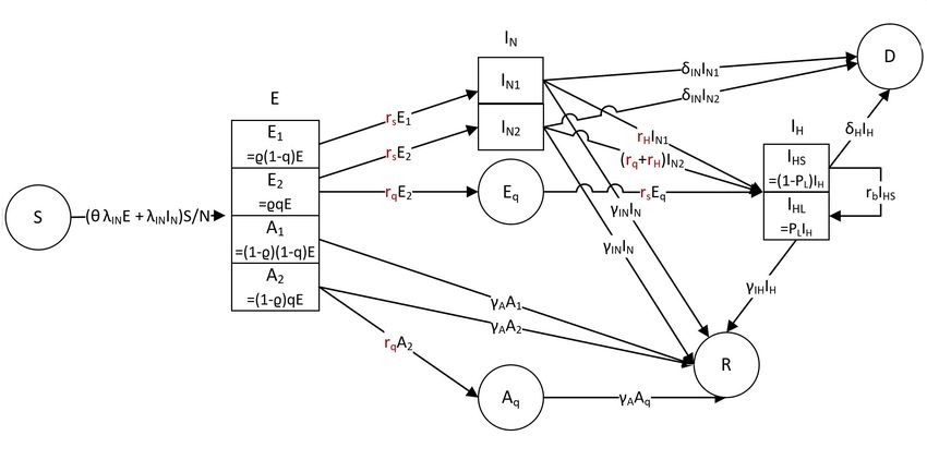
setting for the time varying function is used, that is, λIN (t) = 1{tT1 } aλIN0
and γIH (t) = 1{tT2 } γIH0 . The time T1 is set to be January 29 as there is an
obvious change of rates occurred on January 29 illustrated in Figure 3 (You et al., 2020).
We use observed RH (t+1)−R
IH(t)
H (t)
to approximate γIH on day t. The time T2 is selected to be
the time when γIH has a significant change for each province/city.
The likelihood function is obtained by assuming that daily confirmed cases and recov-
eries are independent Poisson random variables (Wu et al., 2020), that is,
k k ∆Rj
Y e−λi λ∆Hi Y e−γj γj
i
L(λIN , θE , ρ, q, γIH ) =
i=1
∆Hi ! j=1
∆Rj !
where ∆Ht and ∆Rt are the newly confirmed and recovered cases on day t, λt and γt are the
functions of model parameters E(0), IN (0),λIN , θE , ρ, q and γIH based on the Mean-field
Differential Equation System. Parameters are estimated by the posterior means through
the Metropolis-Hastings algorithm implemented in the R package POMP (King et al., 2020,
2016) where non-informative uniform distributions are chosen as the prior distributions, see
Table 1 and 2 for more details.
12medRxiv preprint doi: https://doi.org/10.1101/2020.03.10.20033803. The copyright holder for this preprint (which was not peer-reviewed) is the
author/funder, who has granted medRxiv a license to display the preprint in perpetuity.
It is made available under a CC-BY-NC-ND 4.0 International license .
Table 1: Priors for parameter estimation and values for prefixed parameters
Priors for estimation
Parameter Prior Notes
ρ Uniform(0,1) ρ is the same for all provinces/cities.
θE Uniform(0,1) θ is the same for all provinces/cities.
Combining with the prefixed parameter rH ,
the upper bound of λIN here means R0 is at least 0.7*5,
λIN Uniform(0,0.7) about 3.5,which is a large enough upper bound
based on existing estimates for R0 .
(Wu et al., 2020)
q Uniform(0,1)
a patient should have recovered after a month in hospital,
γIH Uniform(1/30,1)
which means γIH is larger than 1/30.
Existing data show newly infections have begun to decrease.
a Uniform(0,0.2) This means the speed of infection has droped to a relatively
low value, so a should be quite small.
b Uniform(0,1)
Prefixed parameters
Parameter value notes
tmedRxiv preprint doi: https://doi.org/10.1101/2020.03.10.20033803. The copyright holder for this preprint (which was not peer-reviewed) is the
author/funder, who has granted medRxiv a license to display the preprint in perpetuity.
It is made available under a CC-BY-NC-ND 4.0 International license .
Figure 3: Visualization of daily numbers of newly confirmed case along with date, an
obvious change of rate occurred on January 29, 2020.
Table 2: Initial Values
Initial values
City Parameter Prior Notes
E(0) Uniform(0,179)
Beijing
IN (0) Uniform(0,66)
E(0) Uniform(0,136)
Shanghai
IN (0) Uniform(0,50)
Upper bound for IN(0) is obtianed from the
E(0) Uniform(0,424)
Guangdong newly confirmed cases in the first 5 days.
IN (0) Uniform(0,156)
Upper bound for E(0) is obtained from a
E(0) Uniform(0,443)
Zhejiang coarse estimate based on a conservative R0
IN (0) Uniform(0,163)
shown in Wu et al. (2020).
E(0) Uniform(0,275)
Chongqing
IN (0) Uniform(0,101)
E(0) Uniform(0,364)
Hunan
IN (0) Uniform(0,134)
14medRxiv preprint doi: https://doi.org/10.1101/2020.03.10.20033803. The copyright holder for this preprint (which was not peer-reviewed) is the
author/funder, who has granted medRxiv a license to display the preprint in perpetuity.
It is made available under a CC-BY-NC-ND 4.0 International license .
3 Results
3.1 Interpretation of parameters
A summary of the estimated model parameters is given in Table 3, from which we find that
• The estimate of ρ is not sensitive to the choice of γA , about 30% infected individuals
are asymptomatic.
• The estimate of θE is reasonably close to each other with different choices of γA ,
patients with symptoms are about twice as likely to pass a pathogen to others as
asymptomatic patients.
• The estimate of q is not sensitive to the choice of γA except in Shanghai. Zhejiang has
the highest q in the selected regions, which is consistent with the remarkable efforts
made by the The People’s Government of Zhejiang Province (2020), which till March
2, 2020 has successfully tracked more than forty thousand close contacts (People’s
Government of Zhejiang Province (2020)).
The sensitive analysis of γA shows that, (1) the estimates of γIH and b are consistent
regardless the choice of γA as the states RH and IH are both observable; (2) the estimated
initial populations for states E and IN in each regions vary over different choices of γA ,
but are still in the same order of magnitude; (3) the estimate of λIN and a vary with the
choices of γA notably in Guangdong, Zhejiang and Shanghai, cautions need to be taken
when making inferences on λIN and a.
γA = 1/7 γA = 1/10 γA = 1/14
ρ 0.6866 0.7101 0.7077
θ 0.4958 0.4788 0.5459
λgd
IN 0.6120 0.5954 0.5249
λzj
IN 0.4082 0.4018 0.3508
λhn
IN 0.5384 0.5148 0.4412
λbj
IN 0.4882 0.4860 0.4244
λsh
IN 0.4700 0.4890 0.4035
λcq
IN 0.4061 0.4168 0.3724
gd
q 0.4328 0.4747 0.4549
q zj 0.5311 0.527 0.5586
q hn 0.4020 0.4136 0.4087
15medRxiv preprint doi: https://doi.org/10.1101/2020.03.10.20033803. The copyright holder for this preprint (which was not peer-reviewed) is the
author/funder, who has granted medRxiv a license to display the preprint in perpetuity.
It is made available under a CC-BY-NC-ND 4.0 International license .
q bj 0.37365 0.3811 0.3886
q sh 0.4852 0.5411 0.4754
q cq 0.3542 0.3658 0.3827
agd 0.0520 0.0822 0.0597
azj 0.0924 0.0717 0.1096
ahn 0.0276 0.0313 0.0249
abj 0.1113 0.1027 0.1163
sh
a 0.0879 0.1169 0.0642
cq
a 0.1366 0.1310 0.1496
E0gd 152 147 177
E0zj 402 368 398
E0hn 217 222 248
E0bj 43 37 46
E0sh 75 61 75
E0cq 100 69 82
IN0gd 88 83 77
IN0zj 75 79 68
IN0hn 41 39 32
IN0bj 49 49 48
IN0sh 22 23 23
IN0cq 80 86 81
gd
γIH 0.04738 0.04748 0.04735
zj
γIH 0.04856 0.04863 0.04826
hn
γIH 0.07132 0.07071 0.07139
bj
γIH 0.03702 0.03674 0.03707
sh
γIH 0.11650 0.11480 0.11710
cq
γIH 0.06682 0.06838 0.06750
gd
b 0.1732 0.1721 0.1769
bzj 0.3006 0.3078 0.3104
hn
b 0.4556 0.4594 0.4543
bj
b 0.5292 0.5347 0.5195
bsh 0.1558 0.1563 0.1564
bcq 0.2472 0.2419 0.2469
16medRxiv preprint doi: https://doi.org/10.1101/2020.03.10.20033803. The copyright holder for this preprint (which was not peer-reviewed) is the
author/funder, who has granted medRxiv a license to display the preprint in perpetuity.
It is made available under a CC-BY-NC-ND 4.0 International license .
Table 3: parameter estimation
3.2 Prediction of the epidemic trend
Based on the estimated parameters, future trajectories of the epidemic are simulated using
the proposed stochastic dynamic model. For each region, 1000 simulations are conducted to
produce the 95% confidence interval for the epidemic evolution of some key populations. In
this section, the predictions of populations of states, the containment time of the outbreak,
the controlled reproduction number Rc , and a test on the effectiveness of the current medical
tracking policy are reported.
Figure 4 plots the 95% confidence interval of:
• accumulated confirmed cases, namely, the sum of IH, RH and D.
• the population of state IH, representing the people in hospitals.
• population of active virus carriers, consisting of the states E and IN .
Note that the first two populations can be directly observed, but population of E and
IN is not observable. We can see that the observed accumulated confirmed cases and the
population in IH lie in the calculated confidence interval well. Sensitivity analysis shows
that the predicted confidence interval is stable against the uncertainty of γA , which gives
us more confidence in that the proposed model can capture the spread tendency of the
epidemic.
The containment time of the outbreak is defined as the moment when the number of
active virus carriers is first less than a threshold Tc . Noting that the spread of the disease
is due to the existing active virus carriers in the proposed model, thus when the number of
the active virus carriers decreases to a certain level, the new infections are limited, which
means the epidemic is under control. Figure 5 shows the 95% confidence interval of the
containment time of the outbreak for each region when Tc = 10. Among the six regions in
this study, Shanghai is predicted to have the earliest containment time of February 21, while
the containment time in Guangdong is predicted to be the latest, around March 7. From
the daily report of NHC of China, new infections in Shanghai from February 17 to February
21 are 0,0,0,1,0; and new infections in Guangdong in the same period are 6,3,1,1,6, which
potentially supports our prediction. Notice that in sensitivity analysis on γA , we find that
when the recover rate of asymptomatic patients γA gets smaller, the expected containment
time is longer. This is because smaller γA means that infected asymptomatic patients need
17medRxiv preprint doi: https://doi.org/10.1101/2020.03.10.20033803. The copyright holder for this preprint (which was not peer-reviewed) is the
author/funder, who has granted medRxiv a license to display the preprint in perpetuity.
It is made available under a CC-BY-NC-ND 4.0 International license .
more time to recover, which making the number of active virus carriers stays large for a
longer time.
The controlled reproduction number, Rc , reflects the transmission ability of the epi-
demic, which is one of the most important quantities in epidemiology. In this study, the
evolution of Rc is approximated by the ratio between the in-and-out flows of the active virus
carriers in a given time period, that is, for a time interval of length ∆t, say [t, t + ∆t], we
keep tracking the transitions that leads to the increase/decrease of the active virus carrier
population E and IN , with their accumulative numbers recorded. Precisely speaking, we
define
RC IN ([t, t + ∆t]) = card t ∈ [t, t + ∆t], E(t) + IN (t) = E(t−) + IN (t−) + 1
and
RC OU T ([t, t + ∆t]) = card t ∈ [t, t + ∆t], E(t) + IN (t) = E(t−) + IN (t−) − 1 .
Recalling that our stochastic epidemic model evolves as a non-explosive continuous time
Markov process, RC IN (·) and RC OU T (·) are both non-negative finite integers. And
when RC OU T ([t, t + ∆t]) 6= 0, we approximate the controlled reproduction number over
[t, t + ∆t] by its average value
RC IN ([t, t + ∆t])
Rc ([t, t + ∆t]) = .
RC OU T ([t, t + ∆t])
Simulation results for the approximated Rc in each region is shown in Figure 6. In most
provinces and cities we find Rc is between 2 and 3 before control measures, and drops
rapidly to about 0.2 during January 29 and February 1 in all selected regions.
Finally, we evaluate the effectiveness of the current medical tracking policy with a
hypothetical controlled test as follows: while keeping the other parameters we estimated
unchanged, we set the traceable ratio q = 0 to represent the scenario where no medical
tracking were implemented, and let the system evolve. Under this setting, the epidemic
would still be contained, see Figure 7 for details, due to the contact control measures that
reduce the values of λ’s and the reduction of diagnosis waiting time. However, for selected
the provinces and cities in this study, there are significant delays in the dates of containment
when q = 0, which indicates the current medical tracking policy contribute significantly in
containing the epidemic.
4 Discussion
In this article, we propose a novel stochastic dynamic model in order to depict the transmis-
sion mechanism of COVID-19. In comparison with some existing models on COVID-19,
18medRxiv preprint doi: https://doi.org/10.1101/2020.03.10.20033803. The copyright holder for this preprint (which was not peer-reviewed) is the
author/funder, who has granted medRxiv a license to display the preprint in perpetuity.
It is made available under a CC-BY-NC-ND 4.0 International license .
Figure 4: Predicted confidence interval for key populations
19medRxiv preprint doi: https://doi.org/10.1101/2020.03.10.20033803. The copyright holder for this preprint (which was not peer-reviewed) is the
author/funder, who has granted medRxiv a license to display the preprint in perpetuity.
It is made available under a CC-BY-NC-ND 4.0 International license .
Figure 5: Prediction of the containment time of the outbreak. The containment time of
1000 simulations is plotted as a histogram and is fitted with normal distribution for each
region. The y axis represents the density of containment time.
20medRxiv preprint doi: https://doi.org/10.1101/2020.03.10.20033803. The copyright holder for this preprint (which was not peer-reviewed) is the
author/funder, who has granted medRxiv a license to display the preprint in perpetuity.
It is made available under a CC-BY-NC-ND 4.0 International license .
Figure 6: Predicted time-varying Rc curve.
21medRxiv preprint doi: https://doi.org/10.1101/2020.03.10.20033803. The copyright holder for this preprint (which was not peer-reviewed) is the
author/funder, who has granted medRxiv a license to display the preprint in perpetuity.
It is made available under a CC-BY-NC-ND 4.0 International license .
Figure 7: Prediction of the containment time of the outbreak with q = 0. The containment
time of 1000 simulations is plotted as a histogram and is fitted with normal distribution
for each region. The y axis represents the density of containment time.
22medRxiv preprint doi: https://doi.org/10.1101/2020.03.10.20033803. The copyright holder for this preprint (which was not peer-reviewed) is the
author/funder, who has granted medRxiv a license to display the preprint in perpetuity.
It is made available under a CC-BY-NC-ND 4.0 International license .
our model features the employment of a stochastic dynamic as well as a comprehensive
account for the infectious incubation period, the asymptomatic virus carriers, and the
medical tracking measure with time latency, which make it probably closer to reality in
these aspects. Moreover our proposed model also sets the basis for further studies with
individual/network based models, which may not have an exact mean-field counterpart.
In the selected provinces and cities in our study, none of them has more than 2000 accu-
mulated confirmed by now (See Table 5 in Appendix A). The numbers of confirmed cases,
though alerting, are still not comparable to the total populations of these provinces, which
are of the order 10 million-100 million (see Section 2 for exact population data). Moreover,
for a system of size 1000 or so, it is not safe to argue the randomness is negligible due to
the Law of Large Numbers, which makes it already sufficiently close to its hydrodynamic
limit. This justifies the use of stochastic dynamic in our model.
Since the outbreak of COVID-19, the government has conducted large-scale medical
tracking and quarantine measures. These non-negligible measures have a significant impact
on the spread of COVID-19. The sub-states of E, A and IN in our model are able to reflect
such tracking and quarantine measures. Moreover, we also take the latency between medical
tracking and quarantine into account. What’s more, it has been found that the proportion
of asymptomatic infected population is considerable. This justifies the introduction of state
A. Finally, for an exposed and symptomatic individual, this model describes the complete
process from infection to recovery(or death).
In comparison, the model of Tang et al. (2020)(hereafter abbreviated as T.model) failed
to consider the infectivity of the incubative virus carriers(E). What’s more, T.model
assumed quarantine measures will complete at the moment of contact. It is not completely
physical since there should always be a time lag between the transition and the medical
tracking.
In Wu et al. (2020), they didn’t explicitly consider the impact of medical tracking and
quarantine measures in dynamic. As we mentioned above, there are large-scale medical
tracking and quarantine measures after the outbreak of COVID-19, and these measures
have a significant impact on the spread of the virus. The questionable assumption that the
exposed population is non-infectious has also been made in these two models.
The recent work of Yang et al. (2020) proposed a discrete time difference equation(DE)
which correctly accounted the infectious incubation period. However, they assumed a symp-
tomatic patient is hospitalized (“quarantine” in their term, see Page 4 of Yang et al. (2020))
immediately at symptom onset, and did not consider the time lag between symptom onset
diagnosis/hospitalization. Moreover, the probability of transmission b are questionably as-
sumed to be the same for both the symptomatic and asymptomatic population. See Page
3-4 of Yang et al. (2020); and no medical tracking mechanism has been considered. Finally,
23medRxiv preprint doi: https://doi.org/10.1101/2020.03.10.20033803. The copyright holder for this preprint (which was not peer-reviewed) is the
author/funder, who has granted medRxiv a license to display the preprint in perpetuity.
It is made available under a CC-BY-NC-ND 4.0 International license .
there seems to be multiple imperfections in the interpretation of dynamic and estimation
of parameters.
The differences among models mentioned above are hereby summarized in Table 4:
Our Model Tang et al. (2020) Wu et al. (2020) Yang et al. (2020)
Model Type Stochastic ODE ODE (with migration) DE
Infectious Incubation YES NO NO YES
Asymptomatic Carrier YES YES NO NO
Medical Tracking YES YES NO NO
Latency MT∗ YES NO NA NA
Latency H∗∗ YES YES NA NO
Table 4: Comparison of Models
∗ Latency MT= Latency in medical tracking
∗∗ Latency H= Latency in hospitalization
From the estimated parameters, we find that about 30% of the infected are asymp-
tomatic, patients with symptoms are about twice as likely to pass a pathogen to others
as asymptomatic patients, and current containment measures are effective to reduce the
contact and transmission rate. The containment time of the outbreak for different regions
are predicted. Time-varying Rc is calculated and a rapid drop of Rc is observed due to
containment measures that governments take. We have also conducted controlled test and
find that in addition of the control measures reducing the contacts of people, the current
medical tracking policy also contributes significantly in containing the epidemic.
However, we acknowledge there are limitations in the propose model,
1. Given the limited data available, certainly parameters, especially those “far away”
from observation in the proposed model may have a potential risk of identification
issues.
2. The current estimation method converges slowly;
3. The proposed model does not apply if significant changes apply to the current epi-
demic control/treatment measure in the future;
4. The proposed model need further modification if a non-negligible portion of the
asymptomatic patients remain infectious after the end of quarantine.
5. Parameter estimates may lose precision if the stochastic model differs excessively from
its simplification described in Section 4.
24medRxiv preprint doi: https://doi.org/10.1101/2020.03.10.20033803. The copyright holder for this preprint (which was not peer-reviewed) is the
author/funder, who has granted medRxiv a license to display the preprint in perpetuity.
It is made available under a CC-BY-NC-ND 4.0 International license .
In our future study, we propose to complement/generalize our current stochastic model
from the following aspects:
• Improved medical tracking dynamic: In this ongoing work, we are to introduce
a more realistic dynamic for medical tracking. Our current model has already con-
sidered the latency between transmission and quarantine. While in this modification,
medical tracking is triggered in a more physical manner by the affirmative diagnosis
of the transmission source. In this new model the quarantine process of each exposed
agent depends on his/her individual contact history. Thus an individual based, rather
than compartment dynamic is needed. Then the parameters we have estimated can
be used as a basis for the individual-based model.
• Introduction of medical service capacity: In this modification, the maximal
capacity of the medical service system is to be considered, which might be overloaded
when facing a massive outbreak. This idea was first inspired by an Amateur Demon-
stration made by Ele laboratory (2020) on a site named “bilibili”, and seems to be
among the key features of the initial phase of the COVID-19 outbreak in Wuhan.
We may also allow such capacity to be time/configuration dependent to model the
contribution of building the “emergency hospitals” in Wuhan.
• Population flows over cities: We will model the migration of people over different
regions, which could have played an essential role in the spread of the epidemic before
the Chinese New Year of 2020. We will also consider the transmissions on board and
even allow the population flow to react on the information they have about the
epidemic situation.
Acknowledgment
This research is supported by National Natural Science Foundation of China grant 8204100362
and Zhejiang University special scientific research fund for COVID-19 prevention and con-
trol.
References
Athreya, K. B. and Ney, P. E. (1972). Branching processes. Springer-Verlag, New York-
Heidelberg. Die Grundlehren der mathematischen Wissenschaften, Band 196.
Bailey, N. T. J. (1975). The mathematical theory of infectious diseases and its applications.
Hafner Press [Macmillan Publishing Co., Inc.] New York, second edition.
25medRxiv preprint doi: https://doi.org/10.1101/2020.03.10.20033803. The copyright holder for this preprint (which was not peer-reviewed) is the
author/funder, who has granted medRxiv a license to display the preprint in perpetuity.
It is made available under a CC-BY-NC-ND 4.0 International license .
Balcan, D., Colizza, V., Gonçalves, B., Hu, H., Ramasco, J. J., and Vespignani, A. (2009).
Multiscale mobility networks and the spatial spreading of infectious diseases. Proceedings
of the National Academy of Sciences, 106(51):21484–21489.
Barbour, A. D. (1972). The principle of the diffusion of arbitrary constants. J. Appl.
Probability, 9:519–541.
Beijing Municipal Health Commission (2020). Situation report (in chinese). Available at
http://wjw.beijing.gov.cn/xwzx_20031/xwfb/202003/t20200305_1679143.html.
Berrhazi, B.-e., El Fatini, M., Laaribi, A., Pettersson, R., and Taki, R. (2017). A stochastic
SIRS epidemic model incorporating media coverage and driven by Lévy noise. Chaos
Solitons Fractals, 105:60–68.
China National Bureau of Statistics (2018). Annual data by province (in chinese).
Available at http://data.stats.gov.cn/easyquery.htm?cn=E0103&zb=A0301®=
440000&sj=2018.
Chinazzi, M., Davis, J. T., Ajelli, M., Gioannini, C., Litvinova, M., Merler, S., Pastore y
Piontti, A., Mu, K., Rossi, L., Sun, K., Viboud, C., Xiong, X., Yu, H., Halloran, M. E.,
Longini, I. M., and Vespignani, A. (2020). The effect of travel restrictions on the spread
of the 2019 novel coronavirus (covid-19) outbreak. Science.
Chongqing Municipal Health Commission (2020). Situation report (in chinese). Available
at http://wsjkw.cq.gov.cn/yqxxyqtb/20200221/255637.html.
Clémençon, S., Tran, V. C., and de Arazoza, H. (2008). A stochastic SIR model with
contact-tracing: large population limits and statistical inference. J. Biol. Dyn., 2(4):392–
414.
Da Prato, G. and Zabczyk, J. (2014). Stochastic equations in infinite dimensions, volume
152 of Encyclopedia of Mathematics and its Applications. Cambridge University Press,
Cambridge, second edition.
Durrett, R. (1988). Lecture notes on particle systems and percolation. The Wadsworth &
Brooks/Cole Statistics/Probability Series. Wadsworth & Brooks/Cole Advanced Books
& Software, Pacific Grove, CA.
Ele laboratory (2020). Computer simulation programs tell you why it’s not time to go
out now. Available at https://www.bilibili.com/video/av86478875/?spm_id_from=
333.788.b_7265636f5f6c697374.2.
26medRxiv preprint doi: https://doi.org/10.1101/2020.03.10.20033803. The copyright holder for this preprint (which was not peer-reviewed) is the
author/funder, who has granted medRxiv a license to display the preprint in perpetuity.
It is made available under a CC-BY-NC-ND 4.0 International license .
Ethier, S. N. and Kurtz, T. G. (1986). Markov processes. Wiley Series in Probability and
Mathematical Statistics: Probability and Mathematical Statistics. John Wiley & Sons,
Inc., New York. Characterization and convergence.
Government of the People’s Republic of China (2020). Notice of the pneumonia outbreak
prevention and control command of new coronary virus infection in wuhan (in chinese).
Available at http://www.gov.cn/xinwen/2020-01/23/content_5471751.htm.
Health Commission of Guangdong Province (2020). Situation report on new coronavirus
pneumonia outbreak in guangdong province (in chinese). Available at http://wsjkw.
gd.gov.cn/zwyw_yqxx/content/post_2903465.html.
Health Commission of Hunan Province (2020). Situation report on new coronavirus pneu-
monia outbreak in hunan province (in chinese). Available at http://wjw.hunan.gov.
cn/wjw/xxgk/gzdt/zyxw_1/202002/t20200221_11187516.html.
Health Commission of Zhejiang Province (2020). Situation report on new coronavirus
pneumonia outbreak in guangdong province (in chinese). Available at http://www.
zjwjw.gov.cn/art/2020/2/21/art_1202101_41958074.html.
Information Office of Hubei Provincial People’s Government (2020). ”prevention and
control of pneumonia outbreak of new coronary virus infection” press conference (in
chinese). Available at https://www.hubei.gov.cn/hbfb/xwfbh/202002/t20200210_
2023490.shtml.
Japanese Ministry of Health, Labour and Welfare (2020). About the new-style coronavirus
infectious disease which was checked in the cruise ship which is being quarantined at
yokohama port (in japanese). Available at https://www.mhlw.go.jp/stf/newpage_
09668.html.
Ji, C. and Jiang, D. (2014). Threshold behaviour of a stochastic SIR model. Appl. Math.
Model., 38(21-22):5067–5079.
Kendall, D. G. (1956). Deterministic and stochastic epidemics in closed populations.
In Proceedings of the Third Berkeley Symposium on Mathematical Statistics and
Probability, 1954–1955, vol. IV, pages 149–165. University of California Press, Berke-
ley and Los Angeles.
Kermack, W. O. and McKendrick, A. G. (1927). A contribution to the mathematical theory
of epidemics. Proceedings of the Royal Society of London. Series A, Containing Papers
of a Mathematical and Physical Character, 115(772):700–721.
27You can also read