The HBV.IANIGLA Hydrological Model - The R Journal
←
→
Page content transcription
If your browser does not render page correctly, please read the page content below
C ONTRIBUTED R ESEARCH A RTICLES                                                                                      378

           The HBV.IANIGLA Hydrological Model
           by Ezequiel Toum, Mariano H. Masiokas, Ricardo Villalba, Pierre Pitte and Lucas Ruiz

           Abstract Over the past 40 years, the HBV (Hydrologiska Byråns Vattenbalansavdelning) hydrological
           model has been one of the most used worldwide due to its robustness, simplicity, and reliable results.
           Despite these advantages, the available versions impose some limitations for research studies in
           mountain watersheds dominated by ice-snow melt runoff (i.e., no glacier module, a limited number of
           elevation bands, among other constraints). Here we present HBV.IANIGLA, a tool for hydroclimatic
           studies in regions with steep topography and/or cryospheric processes which provides a modular
           and extended implementation of the HBV model as an R package. To our knowledge, this is the first
           modular version of the original HBV model. This feature can be very useful for teaching hydrological
           modeling, as it offers the possibility to build a customized, open-source model that can be adjusted to
           different requirements of students and users.

           Introduction

           Hydrological modeling is widely used by engineers, meteorologists, geographers, geologists, and
           researchers interested in knowing the runoff of rivers in the coming days or the variations of the
           snowpack under certain temperature or precipitation changes, among many other hydrological
           processes.
           The Swedish Meteorological and Hydrological Institute (SMHI) ran the first successful simulation
           of the HBV model in 1972. It was developed to forecast river runoff for hydropower generation in
           Sweden (Bergström and Lindström, 2015). Up to now, many versions have been developed: HBV-ETH
           (Switzerland - Braun and Renner (1992) ), HBV-Light (Switzerland - Seibert and Vis (2012) ), HBV-D
           (Germany - Krysanova et al. (1999) ), HBV-CE (Canada - Stahl et al. (2008) ), TUWmodel (Austria -
           Viglione and Parajka (2016) ), among others. Despite all these free versions, none of them allows the
           users to build their own model using a self-defined combination of modules.
               Buytaert et al. (2008) identified some prerequisites for hydrological model development: (1)
           accessibility in order to reproduce experimental results; (2) modularity as a key element for the devel-
           opment of new ‘ad-hoc’ models to evaluate several aspects of the hydrological cycle and to propose
           improvements; (3) portability, so the model can run in many operating systems; and (4) open-source
           code as a fundamental scientific requirement that allows users to revise, correct, and suggest code
           improvements.
               Slater et al. (2019) highlighted some of the key R packages for hydrological modeling; TUWmodel
           is an R version of the HBV model originally written in Fortran (Viglione and Parajka, 2016); topmodel
           and dynatopmodel are the R versions of the well-known semi-distributed models TOPMODEL and
           Dynamic TOPMODEL (Buytaert, 2018; Metcalfe et al., 2015); airGR (Coron et al., 2017, 2020) includes
           several conceptual rainfall-runoff models, a snow accumulation and melt model and the associated
           functions for their calibration and evaluation; finally, hydromad (Andrews et al., 2011) provides
           a modeling framework for environmental hydrology through water balance accounting and flow
           routing in spatially aggregated catchments.
               Of the models mentioned above, only airGR, hydromad, and TUWmodel present a snow routine
           to account for accumulation and melting processes (temperature index model), but none of them have
           routines to account for glacier mass balance. On the other hand, the glacierSMBM package (Groos
           and Mayer, 2017) allows the modeling of glacier surface mass balance in a fully distributed manner,
           but it was designed to work on the mass balance of a single glacier and to run on a raster-based grid,
           two aspects that limit its applicability at the basin scale.
               The HBV.IANIGLA (Toum, 2021) package was built with the aim of providing a modular hydro-
           logical model approach that adds to the classic HBV routines functions for the modeling of the surface
           mass balance of clean and debris-covered glaciers, a fundamental aspect in the hydrological cycle of
           cold regions of the Andes (Masiokas et al., 2020). The main objective of this article is to present the
           HBV.IANIGLA model structure through its implementation as an R package to serve as a practical
           guide to better understand how it works. The paper is organized as follows:

              • In the next section, we describe the modeling philosophy under HBV and justify the use of a
                modular approach. We then present the HBV.IANIGLA modules and related equations (with
                some conceptual drawings). We end this section with a small study on model computation
                times, a fundamental aspect for sensitivity and uncertainty analysis.
              • Following the methodology, we focus on two examples: on a synthetic basin and on glacier
                mass balance. The reader will find more reproducible examples in the package vignettes.

           The R Journal Vol. 13/1, June 2021                                                   ISSN 2073-4859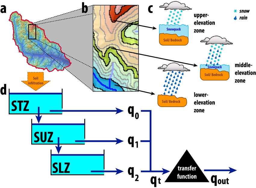
C ONTRIBUTED R ESEARCH A RTICLES                                                                                         379

              • Finally, we condense the key points of the current version of HBV.IANIGLA and propose future
                improvements.

           The HBV.IANIGLA model

           The HBV model

           The HBV model has been used for 40 years for hydrological studies in mountain regions around
           the world (Bergström and Lindström, 2015). The model requires relatively few data inputs (air
           temperature, precipitation, and potential evapotranspiration), which makes it very appropriate in
           scarce data regions such as the Southern Andes. It has been well-documented by other authors (Seibert
           and Vis, 2012; Parajka and Blöschl, 2008; Stahl et al., 2008), a feature that facilitates writing new codes
           and modifying or improving existing equations. Also , it is a bucket-type model with relatively few
           free parameters to calibrate.
               The HBV.IANIGLA version not only takes into account precipitation phase partitioning, snow
           accumulation and melting, actual evaporation and streamflow discharge, but also incorporates a
           module for simulating the surface mass balance of clean and debris-covered glaciers and another
           module for glacier-melt routing. In addition, the package has been designed in a modular fashion,
           allowing users to build their own model. To our knowledge, this is the first HBV version and R
           hydro-modeling package to combine these two features.

           General modeling philosophy

           According to Bergström and Lindström (2015), the HBV model was inspired in the works developed
           in the early 1970s by Nash and Sutcliffe (1970), O’Connell et al. (1970), and Mandeville et al. (1970).
           The primary objective of this model was operational: to forecast streamflow discharge for the Swedish
           hydropower industry. This overriding requirement dictated the characteristics of the model: it
           should not be too complex but physically sound; the input data should conform to standard Swedish
           meteorological measurements; the number of free parameters should be kept to a minimum; and it
           should be easy to understand.
               The above features and lessons learned over more than two decades (Bergström, 1991) resulted
           in a hydrological model composed of four modules: (1) a temperature index model with an air
           temperature-based precipitation partitioning algorithm; (2) a soil moisture routine with a nonlinear
           empirical algorithm to account for abstractions, actual evaporation, and antecedent conditions; (3) a
           bucket-type model (many variants exist up to now) to simulate the catchment storage effect; and (4) a
           transfer function to adjust the timing of the hydrograph to the observed discharge.
               To date, the model has not only been used in operational hydrology but also in scientific research.
           Konz and Seibert (2010) used the HBV-Light version in three alpine catchments in Switzerland and
           Austria to show the value of glacier mass balances in constraining uncertainty in the parameter
           estimation of conceptual models such as HBV. Ali et al. (2018) also applied HBV-Light to evaluate
           model performance in a climate change context in the snow- and ice-dominated Hunza River basin in
           the Karakoram Mountains, Pakistan. Finger et al. (2015) compared model performance in simulations
           of increasing complexity for glacier mass balance and streamflow at the outflow of three Swiss
           watersheds. Stahl et al. (2008) used HBV-CE to estimate streamflow sensitivity to different climate
           change scenarios in British Columbia, Canada. Staudinger et al. (2017) studied the variation of water
           storage with elevation in 21 Swiss alpine and pre-alpine catchments using four different methods:
           water balance analysis, flow recession analysis, calibration of the HBV model, and calibration of
           a transfer function hydrograph separation model using stable isotope observations. In another
           interesting application, Ren et al. (2018) combined HBV with a Bayesian neural network to improve
           seasonal water supply forecasting in the Yarkant River basin, Central Asia. Therefore, the original
           conception of HBV and its evolution have made it a longstanding multipurpose tool for a diverse and
           dynamic user community.

           Modules and equations

           Models are based on a perceptual conception of the basin’s functioning. This perception leads to the
           decision of the equations (hydrological processes) and the construction of a conceptual model (Beven,
           2012). In the HBV.IANIGLA model, these first two stages have already been decided, as the equations
           and coding are in the package, but the user still has a choice on how the watershed or glacier will
           be discretized (in terms of land use and spatial aggregation) and on how the different modules will
           be assembled. This decision should be guided by the objective of the project, the knowledge of the

           The R Journal Vol. 13/1, June 2021                                                      ISSN 2073-4859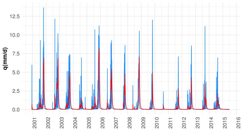
C ONTRIBUTED R ESEARCH A RTICLES                                                                                         380

           hydrological driving process at the chosen modeling scale, and the data available not only for the
           implementation but also for the model evaluation.

           Figure 1: Example of HBV.IANIGLA module assembly in a mountain basin. To account for snow
           accumulation and snowmelt, the basin has been discretized into elevation bands (a and b). Each of
           these polygons has snow and soil routine (c), the effective soil recharge, weighted according to the
           relative area of the elevation band, is passed to the bucket model (d). Finally, the river runoff timing is
           adjusted by a triangular transfer function.

               The following lines describe the modules that must be assembled to build a complete HBV.IANIGLA
           hydrological model. There are three other functions within the package: PET, Pecip_model, and Temp_
           model. The first function contains a potential evapotranspiration model that provides a simple and
           straightforward way to calculate one of the inputs to the soil routine. However, for real-world applica-
           tions we strongly recommend the use of the specialized Evapotranspiration package (Guo et al., 2020).
           The other two functions are linear models to extrapolate air temperature and precipitation records.
           Since we consider that their use is straightforward, we refer the user to the package manual.

           Snow and ice melt models – SnowGlacier_HBV()

           Precipitation is considered to be either snow or rain, depending on whether the temperature is above
           or below a threshold temperature Tr (ºC).

                                              Prain = P              if   Tair > Tr
                                                                                                                   (1)
                                             Psnow = P ∗ SFCF        if   Tair ≤ Tr

           After partitioning, the snowfall is corrected using the SFCF parameter to account for the under-capture
           effect of the precipitation gauge on snow events.
               This function uses a temperature index approach for snow and glacier melt simulation. This kind
           of approximation has been widely used in snow hydrology and glaciology, and different formulations
           have emerged (Hock, 2003; Seibert and Vis, 2012; Braun and Renner, 1992). The temperature index
           formulation takes into account the strong correlation between snow line retreat and accumulated
           temperatures above a certain threshold (with typical values around 0ºC). Hence although many
           authors have proposed more complex formulations (e.g., HBV-Light uses a refreezing and liquid
           retention factor) or even a radiation term (Pellicciotti et al., 2005), this empirical formulation must be
           parsimonious to avoid problems of overparameterization (Kirchner, 2006).

           The R Journal Vol. 13/1, June 2021                                                      ISSN 2073-4859
C ONTRIBUTED R ESEARCH A RTICLES 381
Melt = ( Tair − Tt) ∗ f x if Tair > Tt, (2)
where Tair is the measured or estimated air temperature, Tt is the melting temperature, and f x is a
generic expression of melting factors for snow, clean, or debris-covered ice.
If the air temperature is above the threshold (Tt), melting occurs at a rate proportional to the
melting factor ( f x ). Both the temperature threshold and the melting factor are parameters that must be
calibrated by the user. Note that the time units depend on the resolution of the input data. Although
the examples shown in this article are in a daily time step, the model can be used in the hourly or
monthly resolution. In the next lines, we will describe in detail the different arguments of the function.
The model argument presents three options:
1. Temperature index model: this model is described by equation 2. Here, the user can apply the
most common and recommended set of temperature index formulations.
2. Temperature index model with variable snow cover area: this option is an attempt to offer,
within the package, the same temperature index model as in the Snowmelt Runoff Model
(DeWalle and Rango, 2008). However, this routine has certain limitation: the snow cover series
forces the model to simulate a total effective value (e.g., snow water equivalent), which is not
in-line with the original idea of modeling in elevation bands, where average values are expected.
3. Temperature index model with a variable glacier area: this routine explicitly takes into account
the change in glacier area. Since the automatic reduction of glacier area forces the simulation to
the observed values, the user should evaluate the correspondence between the simulated and
observed mass balances.
The package documentation contains all the necessary information (vignettes with reproducible
examples included) to correctly construct the inputData argument. The data matrix must not contain
missing values (NA's) because HBV.IANIGLA is a continuous hydrological model, meaning that it
simulates all the variables in every time step.
The initial conditions of the model are (initCond):
1. Initial snow water equivalent: this is a state variable, whose initial value will be used in the first
loop. Unless field data is available, it is recommended to use a zero value. Because uncertainties
are common in the initial state variables of the model, it is recommended to use a warm-up
period (between one and two years in daily time step modeling). If the period covered by the
data is very limited, these same values can be used as calibration parameters.
2. Numeric integer indicating the surface type: 1: clean ice; 2: soil; 3: debris-covered ice.
HBV.IANIGLA uses this argument to know which parameters (param argument) to look for. It
also constrains the function output.
3. Area of the glacier(s) (in the elevation band) relative to the basin: this is required only if the
surface is a clean or debris-covered glacier. The area is used to scale the total amount of water
produced (rainfall plus melted water) according to the area of the polygon in the basin. Thus, if
the area of this portion of the glacier corresponds to 5% of the basin area, a value of 0.05 should
be assigned.
The last argument is a numeric vector that stores the parameter values (param) of the modules. For
debris-covered glaciers, a dummy value for the clean glacier melting factor ( f ic ) must be supplied.
This value will not be used internally but simplifies the calibration exercise when working in a basin
with both types of glaciers.
It should be noted that this function allows the construction of a single and lumped simulation.
In order to develop the model for the example shown in figure 1, it will be necessary to build the
model by running the function once per every elevation band (see examples in vignette(package =
"HBV.IANIGLA")).
Soil routine – Soil_HBV()
This routine is based on an empirical formulation that takes into account actual evapotranspiration,
antecedent conditions, and effective soil infiltration. This relationship is described by the so-called
beta function (Bergström and Lindström, 2015),
β
SM
In f = ( Melt + Rain f all ) ∗ , (3)
FC
The R Journal Vol. 13/1, June 2021 ISSN 2073-4859C ONTRIBUTED R ESEARCH A RTICLES 382
where In f is the soil box infiltration, SM is the soil moisture state variable, and β is a nonlinear
parameter between the total amount of water entering the soil box, soil moisture storage, and runoff
generation. This equation is not unique among bucket-type hydrological models. A similar formulation
can be found in the VIC model (Liang et al., 1994). HBV.IANIGLA assumes that all evapotranspiration
occurs from the soil box, so this function implicitly accounts for all abstractions:
SM
Eact = E pot ∗ min ; 1.00 , (4)
FC ∗ LP
where Eact is the actual evapotranspiration, E pot is the potential evapotranspiration, FC is the soil box
water capacity parameter, and LP is a reduction factor.
This type of relationship between potential, actual evapotranspiration, and soil moisture content
has been found by Zhang et al. (2003) in eastern Asia, suggesting that despite its empirical formulation,
in some places, it could have some physical meaning. Finally, and similar to the snow and ice melt
modules, this routine represents a single and lumped simulation.
Routine module – Routing_HBV()
After infiltration, the water follows several complex pathways to streams (McDonnell, 2003). A
detailed description and modeling of these water pathways requires field data and measurements
that are generally not available. An early engineering-based solution to this issue was to consider
this multi-causal delay as a water storage effect at the catchment scale (Dooge, 1973). This practical
modeling approach could be seen as series of linearly interconnected and interrelated reservoirs
(Sivapalan and Blöschl, 2017).
The current HBV.IANIGLA (version 0.2.1) has five different bucket formulations, which are
selected by changing the model argument number (figure 2). To solve the time step change in the
bucket water storage, we used the explicit finite difference form of the mass balance equation over a
discrete-time step (Beven, 2012). Although the general solution has been implemented for a single
linear reservoir (figure 3), we provide solutions for the five-bucket models.
(a) Model 1 (b) Model 2
Figure 2: Diagrams for two of the five available bucket models. The reader will find all the diagrams
in the help menu (?Routing_HBV).
Figure 3: General outline for a water reservoir.
The R Journal Vol. 13/1, June 2021 ISSN 2073-4859C ONTRIBUTED R ESEARCH A RTICLES 383
dS
= u−Q mass balance equation (5)
dt
Q = K∗S continuity equation (6)
from (6),
Q
S= = T∗Q (7)
K
we replace (7) into (5),
dQ
T∗ = u∗Q
dt
In discrete time steps, we use the explicit finite difference form,
Qt − Qt−∆t u − Qt−∆t
= t
∆t T
∆t ∆t
Qt = ∗ ut + (1 − ) ∗ Qt−∆t
T T
∆t
a = (1 − )
T
∆t
b=
T
Qt = a ∗ Qt−∆t + b ∗ ut (8)
St − St−∆t
= ut − Qt−∆t
∆t
St = St−∆t + ∆t ∗ (ut − Qt−∆t ) (9)
Glacier routine module – Glacier_Disch()
Following an approach similar to previous routines, we adopt bucket storage and release scheme
(Jansson et al., 2003). In HBV.IANIGLA, we use the approach proposed by Stahl et al. (2008) for the
HBV-EC model, employed to estimate glacier and streamflow responses to future climate scenarios in
the Bridge River Basin (British Columbia, Canada). The glacier outflow is calculated as:
Figure 4: The glacier runoff release (precipitation plus snow and ice melt) is modeled as a linear water
reservoir with a variable storage coefficient (KG ), which is a function of the snow water equivalent
above the ice body.
KG = KGmin + dKG ∗ exp (SWE/AG ) (10)
q G = KG ∗ SG , (11)
where KG is the actual glacier outflow coefficient, KGmin a minimum storage release coefficient, dKG
the maximum glacier outflow increment, SWE the total snow water equivalent over the glacier, AG a
scaling parameter, SG the glacier water storage, and qG the glacier runoff.
Note that the storage coefficient is a function of a minimum coefficient (denoting poor drainage
conditions on the glacier), the snow water equivalent, and a calibration parameter. When the snowpack
is at its maximum value, drainage occurs at a minimum rate, the opposite occurs in the late summer
when all the snow on the glacier has melted.
For the resolution of the time step change, we also use the explicit finite difference formulation of
the mass balance equation.
The R Journal Vol. 13/1, June 2021 ISSN 2073-4859C ONTRIBUTED R ESEARCH A RTICLES 384
Transfer Function – UH()
To represent the runoff routing in streams, we provide a single parameter triangular function. This
parameter is calibrated to adjust the timing of the simulated river discharge,
Bmax
Q= ∑ Q t − i + 1 ∗ bi , (12)
i =1
where Bmax is the base of the triangular weighting function, bi is the weight for the ith step, and Qt−i+1
is the sum of the glacier and soil bucket runoff.
Computation times
The HBV.IANIGLA functions were written using Rcpp (Eddelbuettel, 2013; Eddelbuettel et al., 2019),
a package that extends the R language using C++. This approach combines the speed and efficiency of
C++, a compiled language, with the powerful interactive environment of R (see table 1), a language
where it is easy to implement specific hydrological workflows (from data retrieval to results analysis)
in a single environment (Slater et al., 2019).
min lq mean median uq max
1.79 1.95 2.65 2.01 2.19 55.81
Table 1: Summary of computation times (in milliseconds) over 1000 runs of the glacier_hbv function
(see vignette("alerce_mass_balance")) . The glacier was discretized into 8 elevation bands (∼ 100
m range). The model was built with the modules Temp_model, Precip_model, and SnowGlacier and
was run on a daily time step over a period of almost 9 years (from 2010-01-01 to 2018-05-30). The
analysis was performed on a CPU with an Intel Core i7-4790 processor at 3.60GHz, on a 64-bit OS
running Ubuntu 18.04 using the microbechmark package (Mersmann, 2019).
Speed is an important issue for hydrological models, as it allows the user to perform not only
uncertainty and sensitivity analysis in reasonable times, but also to apply demanding optimization
algorithms such as DEoptim (Ardia et al., 2016) or different model structures. This is a recommended
practice in the field of hydrological modeling (Beven, 2006, 2008; Pianosi et al., 2016). In addition, the
package only depends on Rcpp (v 0.12.0), a fact that supports its long-term maintenance.
If the reader is interested in comparing the computation times of different R hydrological models we
recommend the work of Astagneau et al. (2020).
Case studies
Lumped synthetic catchment
As a first attempt at applying HBV.IANIGLA, a synthetic lumped catchment (the simplest hydrological
model) is used to introduce the construction of the model and to present a basin discharge calibration
exercise.
Initially, the dataset containing: date, air temperature, precipitation, potential evapotranspiration,
and the catchment outflow is loaded, and then the model construction is conducted (from top to
bottom).
library(HBV.IANIGLA)
# load the lumped catchment dataset
data("lumped_hbv")
# take a look at our dataset
head(lumped_hbv)
summary(lumped_hbv)
For a basin without glaciers, the SnowGlacier module is used only with soil as the underlying
surface. In this exercise, we provide the correct initial conditions and parameters for all modules
except the Routing_HBV function. Consistent with the development of hydrologic models, we build our
The R Journal Vol. 13/1, June 2021 ISSN 2073-4859C ONTRIBUTED R ESEARCH A RTICLES 385
model in a top-down direction, from precipitation to streamflow routing (note that most hydrological
books are structured in the same way).
# consider the SnowGlacier module to take into account
# precipitation partitioning and the snow accumulation/melting.
snow_moduleC ONTRIBUTED R ESEARCH A RTICLES 386
Figure 5: Observed (red) and simulated (blue) basin discharge. Note that the simulation does not
precisely reproduce the observed basin discharge, suggesting that the model needs some calibration.
more information on this example, including the construction of an HBV model as a function and how
to run a sensitivity analysis.
Semi-distributed glacier mass balance
In mountain areas with scarce meteorological information, temperature index models are widely
used to simulate snow and ice melting (Hock, 2003; Konz and Seibert, 2010; Finger et al., 2015; Ayala
et al., 2017). Since air temperature is the most readily available meteorological data in remote areas,
the temperature index approach has been widely used in glaciological and hydrological modeling
(Ohmura, 2001). This package has been built with the SnowGlacier_HBV function, a module that uses
this empirical approach to simulate snow, clean ice, and debris-covered melting.
In this section, we simulate the glacier mass balance for the Alerce glacier. Located on Monte
Tronador (41.15º S ; 71.88º W), nearby the border between Argentina and Chile in the Andes of
Northern Patagonia, Alerce is a medium-size mountain glacier with an area of about 2.33 km2 that
ranges between 1629 and 2358 masl showing a SE aspect (Ruiz et al., 2017; IANIGLA-ING, 2018).
Since 2013, the Alerce glacier has been part of the monitoring network of the National Glacier
Inventory (IANIGLA-ING, 2010). Measurements are conducted following the glaciological method for
seasonal mass balance computation (Kaser et al., 2003). Puerto Montt precipitation (Dirección General
de Aguas, Chile) and Bariloche air temperature (Servicio Meteorológico Nacional - Argentina) were used as
meteorological records to simulate the annual mass balance of the glacier (data(alerce_data)).
When calibrating the model parameters, simulations showing an annual mass balance in the range of
MB ± 400 mm were considered acceptable. MB is the annual surface mass balance of the glacier.
## load the dataset
data(alerce_data)
# now extract
meteo_dataC ONTRIBUTED R ESEARCH A RTICLES 387
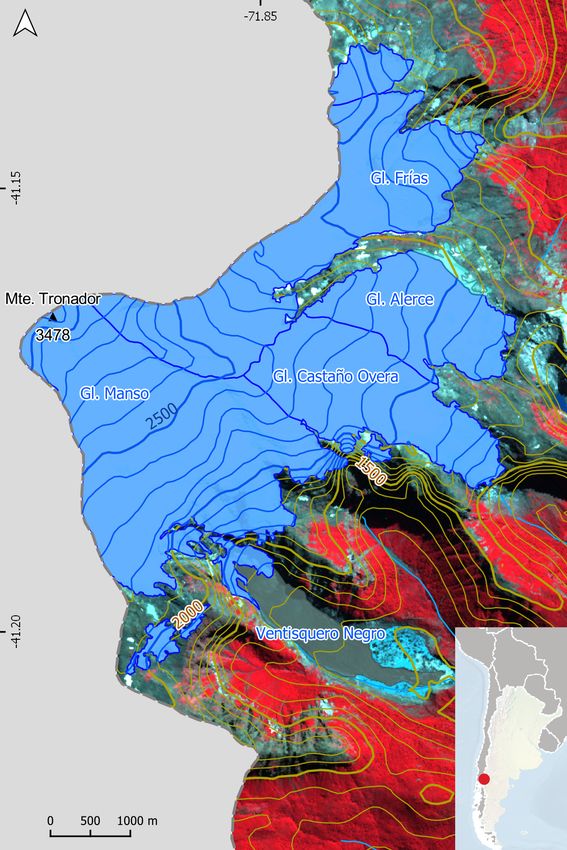
Figure 6: Satellite image of the Monte Tronador showing the location of the main glaciers. The Alerce
glacier, located in the eastern sector, is one of the smallest glaciers at Monte Tronador.
simulations are on different temporal scales), and a goodness-of-fit function (my_gof) were constructed.
The definition of this functions are included in vignette("alerce_mass_balance").
In the following code lines, the sampling strategy for finding acceptable parameter sets is indicated.
# air temperature model
tair_rangeC ONTRIBUTED R ESEARCH A RTICLES 388
n_itC ONTRIBUTED R ESEARCH A RTICLES 389
annual_mbC ONTRIBUTED R ESEARCH A RTICLES 390
Figure 7: Annual mass balances for the period April 2013 - March 2016. All acceptable simulations lies
between the observed uncertainty bounds (despite the fact that we have plot just the mean value).
R-related hydrological packages (e.g., Evapotranspiration, DEoptim, topmodel) or functions (Guo
et al., 2019; Ardia et al., 2016; Buytaert, 2018).
HBV.IANIGLA can also be combined with packages such as tidyverse, sp, raster, hydroGOF, or
plotly to build a single environmental hydrological workflow (Wickham, 2019; Pebesma and Bivand,
2017; Hijmans, 2017; Mauricio Zambrano-Bigiarini, 2017; Sievert et al., 2019). Thus, a hydrological
project can be developed from the beginning to the end in the R environment, facilitating reproducible
and repeatable research (Hutton et al., 2016; Ceola et al., 2015). This type of model design opens up
the possibility for applications beyond the Andes region as well as to incorporate new functions, such
as modules, to explicitly considering the dynamics of glaciers (Huss et al., 2010).
The package functions were built under generic classes (numeric vectors and matrices). This is
an aspect where future improvements can be made. Since HBV.IANIGLA is available in modules, it
could be greatly enhanced using the object-oriented programming (OOP) paradigm. In doing so, the
model could represent an object with properties (e.g., areas, polygons, elevations, among others), and
the HBV routines as part of the methods (functional OOP - S4 types). These methods may also include
(but not limited to): sensitivity and uncertainty analysis, automatic plotting of results, and temporal
aggregation functionality. Even some methods could be recycled from the hydroToolkit OOP package
(Toum, 2020).
The package could also be improved by adding some GUI functionality keeping in mind that in
the words of Chambers (2017), ...extending R is about contributing to the language through applications
designed for a wider audience than the package author itself. Moreover, this objective should not be a target by
its own, but a part or a piece of a bigger project directed to solve real world problems.
Acknowledgements
E.T. acknowledges support from CONICET Argentina through a full-time PhD scholarship. The
constructive suggestions from two anonymous reviewers were very useful for improving the article,
the package documentation, and the vignettes, and are greatly appreciated.
The R Journal Vol. 13/1, June 2021 ISSN 2073-4859C ONTRIBUTED R ESEARCH A RTICLES 391
Bibliography
A. F. Ali, C.-d. Xiao, X.-p. Zhang, M. Adnan, M. Iqbal, and G. Khan. Projection of future streamflow
of the Hunza River Basin, Karakoram Range (Pakistan) using HBV hydrological model. J. Mt.
Sci., 15(10):2218–2235, Oct. 2018. ISSN 1993-0321. doi: 10.1007/s11629-018-4907-4. URL https:
//doi.org/10.1007/s11629-018-4907-4. 0272. [p379]
F. T. Andrews, B. F. W. Croke, and A. J. Jakeman. An open software environment for hydrological
model assessment and development. Environmental Modelling & Software, 26(10):1171–1185, Oct.
2011. ISSN 1364-8152. doi: 10.1016/j.envsoft.2011.04.006. URL http://www.sciencedirect.com/
science/article/pii/S1364815211001046. [p378]
D. Ardia, K. Mullen, B. Peterson, and J. Ulrich. DEoptim: Global Optimization by Differential Evolution,
2016. URL https://CRAN.R-project.org/package=DEoptim. R package version 2.2-4. [p384, 390]
P. C. Astagneau, G. Thirel, O. Delaigue, J. H. A. Guillaume, J. Parajka, C. C. Brauer, A. Viglione,
W. Buytaert, and K. J. Beven. Hydrology modelling R packages: a unified analysis of models
and practicalities from a user perspective. Hydrology and Earth System Sciences Discussions, pages
1–48, Oct. 2020. ISSN 1027-5606. doi: 10.5194/hess-2020-498. URL https://hess.copernicus.org/
preprints/hess-2020-498/. Publisher: Copernicus GmbH. [p384]
A. Ayala, F. Pellicciotti, N. Peleg, and P. Burlando. Melt and surface sublimation across a glacier in a
dry environment: distributed energy-balance modelling of Juncal Norte Glacier, Chile. Journal of
Glaciology, 63(241):803–822, Oct. 2017. ISSN 0022-1430, 1727-5652. doi: 10.1017/jog.2017.46. 0236.
[p386]
S. Bergström. Principles and Confidence in Hydrological Modelling. Hydrology Research, 22(2):123–136,
Apr. 1991. ISSN 0029-1277. doi: 10.2166/nh.1991.0009. URL https://doi.org/10.2166/nh.1991.
0009. [p379]
S. Bergström and G. Lindström. Interpretation of runoff processes in hydrological mod-
elling—experience from the HBV approach. Hydrol. Process., 29(16):3535–3545, July 2015. ISSN
1099-1085. doi: 10.1002/hyp.10510. URL http://onlinelibrary.wiley.com/doi/10.1002/hyp.
10510/abstract. [p378, 379, 381]
K. Beven. A manifesto for the equifinality thesis. Journal of Hydrology, 320(1):18–36, Mar. 2006. ISSN
0022-1694. doi: 10.1016/j.jhydrol.2005.07.007. URL http://www.sciencedirect.com/science/
article/pii/S002216940500332X. 0126. [p384]
K. Beven. Environmental Modelling: An Uncertain Future? CRC Press, London, 1 edition edition, Sept.
2008. ISBN 978-0-415-45759-0. [p384]
K. J. Beven. Rainfall - Runoff Modelling. Wiley, Chichester, 2 edition edition, Mar. 2012. ISBN 978-0-470-
86671-9. [p379, 382]
L. N. Braun and C. B. Renner. Application of a conceptual runoff model in different physiographic
regions of Switzerland. Hydrological Sciences Journal, 37(3):217–231, June 1992. ISSN 0262-6667. doi:
10.1080/02626669209492583. URL https://doi.org/10.1080/02626669209492583. [p378, 380]
W. Buytaert. topmodel: Implementation of the Hydrological Model TOPMODEL in R, 2018. URL https:
//CRAN.R-project.org/package=topmodel. R package version 0.7.3. [p378, 390]
W. Buytaert, D. Reusser, S. Krause, and J.-P. Renaud. Why can’t we do better than Topmodel?
Hydrol. Process., 22(20):4175–4179, Sept. 2008. ISSN 1099-1085. doi: 10.1002/hyp.7125. URL
http://onlinelibrary.wiley.com/doi/10.1002/hyp.7125/abstract. 0208. [p378]
S. Ceola, B. Arheimer, E. Baratti, G. Blöschl, R. Capell, A. Castellarin, J. Freer, D. Han, M. Hrachowitz,
Y. Hundecha, C. Hutton, G. Lindström, A. Montanari, R. Nijzink, J. Parajka, E. Toth, A. Viglione,
and T. Wagener. Virtual laboratories: new opportunities for collaborative water science. Hydrology
and Earth System Sciences, 19(4):2101–2117, Apr. 2015. ISSN 1027-5606. doi: https://doi.org/
10.5194/hess-19-2101-2015. URL https://www.hydrol-earth-syst-sci.net/19/2101/2015/hess-
19-2101-2015.html. [p390]
J. M. Chambers. Extending R. CRC Press, Dec. 2017. ISBN 978-1-4987-7572-4. Google-Books-ID:
kxxjDAAAQBAJ. [p390]
L. Coron, G. Thirel, O. Delaigue, C. Perrin, and V. Andréassian. The suite of lumped GR hydrological
models in an R package. Environmental Modelling and Software, 94:166–171, 2017. doi: 10.1016/j.
envsoft.2017.05.002. [p378]
The R Journal Vol. 13/1, June 2021 ISSN 2073-4859C ONTRIBUTED R ESEARCH A RTICLES 392
L. Coron, O. Delaigue, G. Thirel, C. Perrin, and C. Michel. airGR: Suite of GR Hydrological Models for
Precipitation-Runoff Modelling, 2020. URL https://CRAN.R-project.org/package=airGR. R package
version 1.4.3.65. [p378]
D. R. DeWalle and A. Rango. Principles of Snow Hydrology. Cambridge University Press, Cambridge,
UK ; New York, July 2008. ISBN 978-0-521-82362-3. [p381]
J. Dooge. Linear Theory of Hydrologic Systems. Agricultural Research Service, U.S. Department of
Agriculture, 1973. [p382]
D. Eddelbuettel. Seamless R and C++ Integration with Rcpp. Use R! Springer-Verlag, New York, 2013.
ISBN 978-1-4614-6867-7. URL https://www.springer.com/gp/book/9781461468677. [p384]
D. Eddelbuettel, R. Francois, J. Allaire, K. Ushey, Q. Kou, N. Russell, D. Bates, and J. Chambers. Rcpp:
Seamless R and C++ Integration, 2019. URL https://CRAN.R-project.org/package=Rcpp. R package
version 1.0.2. [p384]
D. Finger, M. Vis, M. Huss, and J. Seibert. The value of multiple data set calibration versus model
complexity for improving the performance of hydrological models in mountain catchments. Water
Resour. Res., 51(4):1939–1958, Apr. 2015. ISSN 1944-7973. doi: 10.1002/2014WR015712. URL
http://onlinelibrary.wiley.com/doi/10.1002/2014WR015712/abstract. [p379, 386]
A. R. Groos and C. Mayer. glacierSMBM: Glacier Surface Mass Balance Model, 2017. URL https:
//CRAN.R-project.org/package=glacierSMBM. R package version 0.1. [p378]
D. Guo, S. Westra, and T. Peterson. Evapotranspiration: Modelling Actual, Potential and Reference
Crop Evapotranspiration, 2019. URL https://CRAN.R-project.org/package=Evapotranspiration.
R package version 1.14. [p390]
D. Guo, S. Westra, and T. Peterson. Evapotranspiration: Modelling Actual, Potential and Reference
Crop Evapotranspiration, 2020. URL https://CRAN.R-project.org/package=Evapotranspiration.
R package version 1.15. [p380]
R. J. Hijmans. raster: Geographic Data Analysis and Modeling, 2017. URL https://CRAN.R-project.org/
package=raster. R package version 2.6-7. [p390]
R. Hock. Temperature index melt modelling in mountain areas. Journal of Hydrology, 282(1):104–115,
Nov. 2003. ISSN 0022-1694. doi: 10.1016/S0022-1694(03)00257-9. URL http://www.sciencedirect.
com/science/article/pii/S0022169403002579. [p380, 386]
M. Huss, G. Jouvet, D. Farinotti, and A. Bauder. Future high-mountain hydrology: a new parame-
terization of glacier retreat. Hydrol. Earth Syst. Sci., 14(5):815–829, May 2010. ISSN 1607-7938. doi:
10.5194/hess-14-815-2010. URL https://www.hydrol-earth-syst-sci.net/14/815/2010/. 0019.
[p390]
C. Hutton, T. Wagener, J. Freer, D. Han, C. Duffy, and B. Arheimer. Most computational hydrology
is not reproducible, so is it really science? Water Resources Research, 52(10):7548–7555, 2016. ISSN
1944-7973. doi: 10.1002/2016WR019285. URL https://agupubs.onlinelibrary.wiley.com/doi/
abs/10.1002/2016WR019285. [p390]
IANIGLA-ING. Inventario Nacional de Glaciares y Ambiente Periglacial:Fundamentos y Cronograma
de Ejecución. Technical report, CONICET, Mendoza, 2010. URL http://www.glaciaresargentinos.
gob.ar/wp-content/uploads/legales/fundamentos_cronograma_ejecucion.pdf. [p386]
IANIGLA-ING. IANIGLA-Inventario Nacional de Glaciares. 2018. Informe de las subcuencas de los
ríos Manso, Villegas y Foyel. Cuenca de los ríos Manso y Puelo. IANIGLA-CONICET, Ministerio
de Ambiente y Desarrollo Sustentable de la Nación. Technical report, IANIGLA, 2018. URL
http://www.glaciaresargentinos.gob.ar. [p386]
P. Jansson, R. Hock, and T. Schneider. The concept of glacier storage: a review. Journal of Hydrology,
282(1):116–129, Nov. 2003. ISSN 0022-1694. doi: 10.1016/S0022-1694(03)00258-0. URL http:
//www.sciencedirect.com/science/article/pii/S0022169403002580. 0229. [p383]
G. Kaser, A. Fountain, and P. Jansson. A manual for monitoring the mass balance of mountain glaciers.
Manual 59, UNESCO, Paris, 2003. URL http://ulis2.unesco.org/images/0012/001295/129593E.
pdf. 0396. [p386]
The R Journal Vol. 13/1, June 2021 ISSN 2073-4859C ONTRIBUTED R ESEARCH A RTICLES 393
J. W. Kirchner. Getting the right answers for the right reasons: Linking measurements, analyses,
and models to advance the science of hydrology. Water Resources Research, 42(3), Mar. 2006. ISSN
1944-7973. doi: 10.1029/2005WR004362. URL https://agupubs.onlinelibrary.wiley.com/doi/
abs/10.1029/2005WR004362. 0216. [p380]
M. Konz and J. Seibert. On the value of glacier mass balances for hydrological model calibration. Journal
of Hydrology, 385(1):238–246, May 2010. ISSN 0022-1694. doi: 10.1016/j.jhydrol.2010.02.025. URL
http://www.sciencedirect.com/science/article/pii/S0022169410000958. 0189. [p379, 386]
V. Krysanova, A. Bronstert, and D.-I. Müller-Wohlfeil. Modelling river discharge for large drainage
basins: from lumped to distributed approach. Hydrological Sciences Journal, 44(2):313–331, Apr.
1999. ISSN 0262-6667. doi: 10.1080/02626669909492224. URL https://doi.org/10.1080/
02626669909492224. [p378]
X. Liang, D. P. Lettenmaier, E. F. Wood, and S. J. Burges. A simple hydrologically based model
of land surface water and energy fluxes for general circulation models. Journal of Geophysi-
cal Research: Atmospheres, 99(D7):14415–14428, 1994. ISSN 2156-2202. doi: https://doi.org/10.
1029/94JD00483. URL https://agupubs.onlinelibrary.wiley.com/doi/abs/10.1029/94JD00483.
_eprint: https://agupubs.onlinelibrary.wiley.com/doi/pdf/10.1029/94JD00483. [p382]
A. N. Mandeville, P. E. O’Connell, J. V. Sutcliffe, and J. E. Nash. River flow forecasting through
conceptual models part III - The Ray catchment at Grendon Underwood. Journal of Hydrology, 11
(2):109–128, Aug. 1970. ISSN 0022-1694. doi: 10.1016/0022-1694(70)90098-3. URL http://www.
sciencedirect.com/science/article/pii/0022169470900983. [p379]
M. H. Masiokas, A. Rabatel, A. Rivera, L. Ruiz, P. Pitte, J. L. Ceballos, G. Barcaza, A. Soruco, F. Bown,
E. Berthier, I. Dussaillant, and S. MacDonell. A Review of the Current State and Recent Changes of
the Andean Cryosphere. Frontiers in Earth Science, 8, 2020. ISSN 2296-6463. doi: 10.3389/feart.2020.
00099. URL https://www.frontiersin.org/articles/10.3389/feart.2020.00099/full. 0424.
[p378]
Mauricio Zambrano-Bigiarini. hydroGOF: Goodness-of-Fit Functions for Comparison of Simulated and
Observed Hydrological Time Series, 2017. URL https://CRAN.R-project.org/package=hydroGOF. R
package version 0.3-10. [p390]
J. J. McDonnell. Where does water go when it rains? Moving beyond the variable source area concept
of rainfall-runoff response. Hydrological Processes, 17(9):1869–1875, 2003. ISSN 1099-1085. doi:
https://doi.org/10.1002/hyp.5132. URL https://onlinelibrary.wiley.com/doi/abs/10.1002/
hyp.5132. _eprint: https://onlinelibrary.wiley.com/doi/pdf/10.1002/hyp.5132. [p382]
O. Mersmann. microbenchmark: Accurate Timing Functions, 2019. URL https://CRAN.R-project.org/
package=microbenchmark. R package version 1.4-7. [p384]
P. Metcalfe, K. Beven, and J. Freer. Dynamic TOPMODEL: A new implementation in R and its sensitivity
to time and space steps. Environmental Modelling & Software, 72:155–172, Oct. 2015. ISSN 1364-8152.
doi: 10.1016/j.envsoft.2015.06.010. URL http://www.sciencedirect.com/science/article/pii/
S1364815215001735. 0306. [p378]
J. E. Nash and J. V. Sutcliffe. River flow forecasting through conceptual models part I — A discussion
of principles. Journal of Hydrology, 10(3):282–290, Apr. 1970. ISSN 0022-1694. doi: 10.1016/0022-
1694(70)90255-6. URL http://www.sciencedirect.com/science/article/pii/0022169470902556.
0004. [p379]
P. E. O’Connell, J. E. Nash, and J. P. Farrell. River flow forecasting through conceptual models part II -
The Brosna catchment at Ferbane. Journal of Hydrology, 10(4):317–329, June 1970. ISSN 0022-1694.
doi: 10.1016/0022-1694(70)90221-0. URL http://www.sciencedirect.com/science/article/pii/
0022169470902210. [p379]
A. Ohmura. Physical basis for the temperature-based melt-index method. Journal of Applied Meteorology,
40(4):753–761, Apr. 2001. ISSN 0894-8763. doi: 10.1175/1520-0450(2001)0402.0.CO;2.
URL https://doi.org/10.1175/1520-0450(2001)0402.0.CO;2. [p386]
J. Parajka and G. Blöschl. The value of MODIS snow cover data in validating and calibrating con-
ceptual hydrologic models. Journal of Hydrology, 358(3):240–258, Sept. 2008. ISSN 0022-1694.
doi: 10.1016/j.jhydrol.2008.06.006. URL http://www.sciencedirect.com/science/article/pii/
S0022169408002862. 0199. [p379]
E. Pebesma and R. Bivand. sp: Classes and Methods for Spatial Data, 2017. URL https://CRAN.R-
project.org/package=sp. R package version 1.2-5. [p390]
The R Journal Vol. 13/1, June 2021 ISSN 2073-4859C ONTRIBUTED R ESEARCH A RTICLES 394
F. Pellicciotti, B. Brock, U. Strasser, P. Burlando, M. Funk, and J. Corripio. An enhanced temperature-
index glacier melt model including the shortwave radiation balance: development and testing for
Haut Glacier d’Arolla, Switzerland. Journal of Glaciology, 51(175):573–587, 2005. ISSN 0022-1430,
1727-5652. doi: 10.3189/172756505781829124. Publisher: Cambridge University Press. [p380]
F. Pianosi, K. Beven, J. Freer, J. W. Hall, J. Rougier, D. B. Stephenson, and T. Wagener. Sensitivity
analysis of environmental models: A systematic review with practical workflow. Environmental
Modelling & Software, 79:214–232, May 2016. ISSN 1364-8152. doi: 10.1016/j.envsoft.2016.02.008. URL
http://www.sciencedirect.com/science/article/pii/S1364815216300287. 0324. [p384, 389]
W. W. Ren, T. Yang, C. S. Huang, C. Y. Xu, and Q. X. Shao. Improving monthly streamflow prediction
in alpine regions: integrating HBV model with Bayesian neural network. Stoch Environ Res Risk
Assess, 32(12):3381–3396, Dec. 2018. ISSN 1436-3259. doi: 10.1007/s00477-018-1553-x. URL https:
//doi.org/10.1007/s00477-018-1553-x. 0359. [p379]
L. Ruiz, E. Berthier, M. Viale, P. Pitte, and M. H. Masiokas. Recent geodetic mass balance of Monte
Tronador glaciers, northern Patagonian Andes. The Cryosphere, 11(1):619–634, Feb. 2017. ISSN
1994-0424. doi: 10.5194/tc-11-619-2017. URL https://www.the-cryosphere.net/11/619/2017/.
0237. [p386]
J. Seibert and M. J. P. Vis. Teaching hydrological modeling with a user-friendly catchment-runoff-
model software package. Hydrol. Earth Syst. Sci., 16(9):3315–3325, Sept. 2012. ISSN 1607-7938. doi:
10.5194/hess-16-3315-2012. URL https://www.hydrol-earth-syst-sci.net/16/3315/2012/. 0021.
[p378, 379, 380]
C. Sievert, C. Parmer, T. Hocking, S. Chamberlain, K. Ram, M. Corvellec, and P. Despouy. plotly: Create
Interactive Web Graphics via ’plotly.js’, 2019. URL https://CRAN.R-project.org/package=plotly. R
package version 4.9.0. [p390]
M. Sivapalan and G. Blöschl. The Growth of Hydrological Understanding: Technologies, Ideas,
and Societal Needs Shape the Field. Water Resources Research, 53(10):8137–8146, 2017. ISSN 1944-
7973. doi: 10.1002/2017WR021396. URL https://agupubs.onlinelibrary.wiley.com/doi/abs/
10.1002/2017WR021396. 0413. [p382]
L. J. Slater, G. Thirel, S. Harrigan, O. Delaigue, A. Hurley, A. Khouakhi, I. Prodoscimi, C. Vitolo, and
K. Smith. Using R in hydrology: a review of recent developments and future directions. Hydrology
and Earth System Sciences Discussions, pages 1–33, Feb. 2019. ISSN 1027-5606. doi: https://doi.org/
10.5194/hess-2019-50. URL https://www.hydrol-earth-syst-sci-discuss.net/hess-2019-50/.
[p378, 384]
K. Stahl, R. D. Moore, J. M. Shea, D. Hutchinson, and A. J. Cannon. Coupled modelling of glacier and
streamflow response to future climate scenarios. Water Resour. Res., 44(2):W02422, Feb. 2008. ISSN
1944-7973. doi: 10.1029/2007WR005956. URL http://onlinelibrary.wiley.com/doi/10.1029/
2007WR005956/abstract. 0013. [p378, 379, 383]
M. Staudinger, M. Stoelzle, S. Seeger, J. Seibert, M. Weiler, and K. Stahl. Catchment water storage
variation with elevation. Hydrological Processes, 31(11):2000–2015, 2017. ISSN 1099-1085. doi:
10.1002/hyp.11158. URL https://onlinelibrary.wiley.com/doi/abs/10.1002/hyp.11158. [p379]
E. Toum. hydroToolkit: Hydrological Tools for Handling Hydro-Meteorological Data from Argentina and Chile,
2020. R package version 0.1.1. [p390]
E. Toum. HBV.IANIGLA: Modular Hydrological Model, 2021. URL https://CRAN.R-project.org/
package=HBV.IANIGLA. 0.2.0. [p378]
A. Viglione and J. Parajka. TUWmodel: Lumped Hydrological Model for Education Purposes, 2016. URL
https://CRAN.R-project.org/package=TUWmodel. R package version 0.1-8. [p378]
H. Wickham. tidyverse: Easily Install and Load the ’Tidyverse’, 2019. URL https://CRAN.R-project.org/
package=tidyverse. R package version 1.3.0. [p390]
Y. Zhang, T. Ohata, K. Ersi, and Y. Tandong. Observation and estimation of evaporation from the
ground surface of the cryosphere in eastern Asia. Hydrological Processes, 17(6):1135–1147, Apr. 2003.
ISSN 1099-1085. doi: 10.1002/hyp.1183. URL http://onlinelibrary.wiley.com/doi/10.1002/
hyp.1183/abstract. [p382]
The R Journal Vol. 13/1, June 2021 ISSN 2073-4859C ONTRIBUTED R ESEARCH A RTICLES 395
Ezequiel Toum
IANIGLA-CONICET
Av. Ruiz Leal s/n Parque General San Martin - Mendoza
Argentina
etoum@mendoza-conicet.gob.ar
Mariano H. Masiokas
IANIGLA-CONICET
Av. Ruiz Leal s/n Parque General San Martin - Mendoza
Argentina
mmasiokas@mendoza-conicet.gob.ar
Ricardo Villalba
IANIGLA-CONICET
Av. Ruiz Leal s/n Parque General San Martin - Mendoza
Argentina
ricardo@mendoza-conicet.gob.ar
Pierre Pitte
IANIGLA-CONICET
Av. Ruiz Leal s/n Parque General San Martin - Mendoza
Argentina
pierrepitte@mendoza-conicet.gob.ar
Lucas Ruiz
IANIGLA-CONICET
Av. Ruiz Leal s/n Parque General San Martin - Mendoza
Argentina
lruiz@mendoza-conicet.gob.ar
The R Journal Vol. 13/1, June 2021 ISSN 2073-4859You can also read