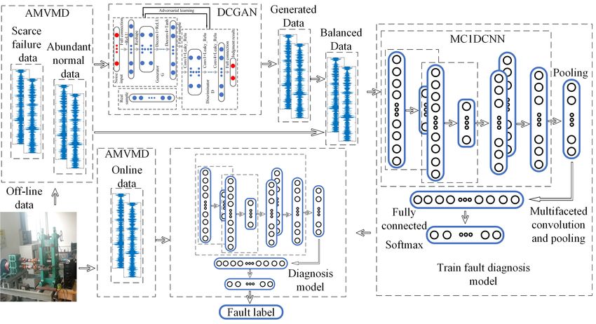
Fault Diagnosis Method for Rolling Mill Multi Row Bearings Based on AMVMD-MC1DCNN under Unbalanced Dataset
←
→
Page content transcription
If your browser does not render page correctly, please read the page content below
sensors
Article
Fault Diagnosis Method for Rolling Mill Multi Row Bearings
Based on AMVMD-MC1DCNN under Unbalanced Dataset
Chen Zhao, Jianliang Sun *, Shuilin Lin and Yan Peng

                                          National Cold Rolling Strip Equipment and Process Engineering Technology Research Center,
                                          Yanshan University, Qinhuangdao 066000, China; zhaochen136@stumail.ysu.edu.cn (C.Z.);
                                          lslin@stumail.ysu.edu.cn (S.L.); pengyan@ysu.edu.cn (Y.P.)
                                          * Correspondence: sunjianliang@ysu.edu.cn; Tel.: +86-137-2255-0756

                                          Abstract: Rolling mill multi-row bearings are subjected to axial loads, which cause damage of rolling
                                          elements and cages, so the axial vibration signal contains rich fault character information. The vertical
                                          shock caused by the failure is weakened because multiple rows of bearings are subjected to radial
                                          forces together. Considering the special characters of rolling mill bearing vibration signals, a fault
                                          diagnosis method combining Adaptive Multivariate Variational Mode Decomposition (AMVMD) and
                                          Multi-channel One-dimensional Convolution Neural Network (MC1DCNN) is proposed to improve
                                          the diagnosis accuracy. Additionally, Deep Convolutional Generative Adversarial Network (DCGAN)
                                          is embedded in models to solve the problem of fault data scarcity. DCGAN is used to generate
                                          AMVMD reconstruction data to supplement the unbalanced dataset, and the MC1DCNN model is
                                          trained by the dataset to diagnose the real data. The proposed method is compared with a variety of
                                          diagnostic models, and the experimental results show that the method can effectively improve the

                                          diagnosis accuracy of rolling mill multi-row bearing under unbalanced dataset conditions. It is an
                                   important guide to the current problem of insufficient data and low diagnosis accuracy faced in the
Citation: Zhao, C.; Sun, J.; Lin, S.;     fault diagnosis of multi-row bearings such as rolling mills.
Peng, Y. Fault Diagnosis Method for
Rolling Mill Multi Row Bearings           Keywords: Adaptive Multivariate Variational Mode Decomposition; Multi-channel One-Dimensional
Based on AMVMD-MC1DCNN                    Convolutional Neural Network; deep convolutional generation adversarial network; unbalanced
under Unbalanced Dataset. Sensors         dataset fault diagnosis; rolling mill multi-row bearings
2021, 21, 5494. https://doi.org/
10.3390/s21165494

Academic Editor: Ruqiang Yan              1. Introduction
                                               Rolling mill multi-row bearings are the core of the main drive system of the rolling
Received: 4 July 2021
Accepted: 11 August 2021
                                          mill, which support the rolling mill roll system and withstand huge radial forces. Under
Published: 15 August 2021
                                          the working conditions, the rolls have axial displacement and roll bending phenomenon,
                                          the bearing can absorb the harmful bending moment and axial force. Therefore, the cage
Publisher’s Note: MDPI stays neutral
                                          and rolling body are the main failure parts of the rolling mill multi-row bearing. Accord-
with regard to jurisdictional claims in
                                          ing to statistics, 30% of rotating machinery failures are caused by bearings, and their
published maps and institutional affil-   operating conditions directly affect system performance [1,2]. If the multi-row bearings
iations.                                  of large machinery such as the rolling mill are damaged, it can lead to long downtime,
                                          and extremely high repair costs and serious economic losses. Therefore, it is necessary to
                                          carry out the diagnosis of bearing faults in large machinery and equipment such as rolling
                                          mills. Due to the harsh factory conditions and noise interference, the vibration signal has
Copyright: © 2021 by the authors.
                                          nonlinear and non-stationary characters [3]. Therefore, conventional time domain wave-
Licensee MDPI, Basel, Switzerland.
                                          form and frequency domain feature fault analysis methods have limitations in bearing
This article is an open access article
                                          fault diagnosis [4].
distributed under the terms and                The time-frequency analysis method has better results in dealing with nonlinear and
conditions of the Creative Commons        non-stationary signals, which has been widely used in fault diagnosis. The following
Attribution (CC BY) license (https://     methods are commonly used: Empirical Mode Decomposition (EMD) [5], Local Mean
creativecommons.org/licenses/by/          Decomposition (LMD) [6], Empirical Wavelet Transform (EWT) [7], Variational Mode De-
4.0/).                                    composition (VMD) [8], etc. Among them, VMD changes the previous signal processing

Sensors 2021, 21, 5494. https://doi.org/10.3390/s21165494                                                  https://www.mdpi.com/journal/sensors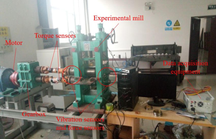
Sensors 2021, 21, 5494                                                                                             2 of 22

                         and decomposes the signal according to the center frequency, which makes the charac-
                         ters of Intrinsic Mode Function (IMF) much more controllable. In [9], Li compared the
                         effectiveness of VMD and EMD in processing vibration signals, which proved that VMD
                         outperforms EMD and can effectively overcome the problem of modal mixing. In [10],
                         Aneesh considered the classification of power quality disturbances based on VMD and EWT,
                         and classification results indicated that VMD outperformed EWT for feature extraction.
                         However, the above algorithms have limitations in processing multidimensional signals,
                         so in [11], Rehman proposed Multivariate Empirical Mode Decomposition (MEMD). Based
                         on the idea of MEMD, in [12], Aftab and Rehman extended VMD to multidimensional and
                         proposed Multivariate Variational Mode Decomposition (MVMD), which effectively solves
                         the problem of synchronous processing of multivariate data. The literature [13] showed
                         that the effect of VMD decomposition was greatly influenced by the parameters K and
                         α, and it cannot achieve adaptive decomposition of the signal in a real sense. Therefore,
                         MVMD as an extension of VMD also has a parameter optimization problem. Although
                         the multiple signal input activates the noise reduction capability of the Wiener filter and
                         reduces the effect of the number of IMF K on the decomposition effect [14], the iterative
                         optimization-seeking process of MVMD converges too slowly, and the decomposition effect
                         is still affected by the penalty factor α.
                               In view of the superior performance of mode decomposition, scholars have combined
                         it with pattern recognition methods to become the mainstream fault diagnosis method.
                         In [15], Isham used VMD to reconstruct wind turbine gearbox vibration signals and ex-
                         tracted multi-domain features that were passed to an Extreme Value Learning Machine
                         (ELM) for fault classification. The ELM requires fewer samples for training and has a
                         fast speed on diagnosis, but the relative stability of the model is weaker [16]. In [17], Gu
                         used MVMD to decompose diesel multi-sensor signals for processing, but still needed
                         to use band entropy for feature extraction in the process of combining Support Vector
                         Machines (SVM). However, the kernel function selection of SVM has a large impact on
                         the classification, and the classification effect is significantly affected by the fault samples.
                         Therefore, SVM often needs to be combined with optimization algorithms, which increases
                         the tediousness of the model [18]. Because conventional classifiers such as ELM and SVM
                         need to be combined with feature extraction methods, the fault diagnosis method deviates
                         from the general trend of end-to-end (signal-to-fault) diagnosis.
                               Convolutional Neural Networks (CNNs) have had significant achievements in the
                         field of image recognition and have become a research hotspot in deep learning [19]. CNN
                         has the function of automatic feature extraction and pattern recognition, which can realize
                         the fault identification of equipment by inputting vibration signal. Therefore, CNN is
                         widely used in end-to-end fault diagnosis. There are two main modes of application of
                         CNN in fault diagnosis. On the one hand, the vibration data is transformed into a two-
                         dimensional data matrix for identification. In [20], Chen transformed a certain length
                         of one-dimensional vibration signal into a two-dimensional matrix and used CNN for
                         fault identification. In [21], Xu used the IMF component signal of VMD as the input
                         of CNN and achieved good results in the fault diagnosis of wind turbine bearings. On
                         the other hand, vibration data can be transformed into image formats such as grayscale
                         images, frequency domain maps and speech spectrum maps for recognition. In [22], Zhu
                         transformed the signal by short-time Fourier transform into a frequency domain map
                         for fault diagnosis by CNN. In [23], Zhao transformed the one-dimensional vibration
                         signal into a two-dimensional grayscale image and achieved diagnostic classification of
                         faults by CNN. However, the vibration signal is a one-dimensional time series signal,
                         and the data at each moment have a certain correlation. Converting one-dimensional
                         data into two-dimensional arrays and performing feature extraction by convolutional
                         kernels can break the spatial correlation of signals, resulting in the loss of fault character
                         information. Therefore, scholars have proposed One-Dimensional Convolutional Neural
                         Network (1DCNN) for the special characteristics of one-dimensional time series. In [24],
                         Levent directly input the raw vibration signal of the bearing into 1DCNN to achieve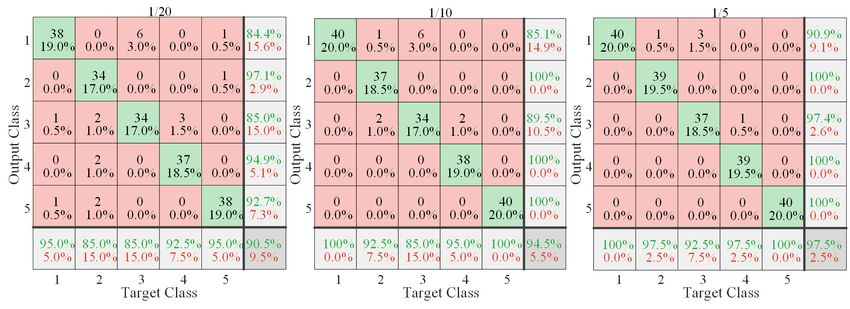
Sensors 2021, 21, 5494                                                                                          3 of 22

                         rapid diagnosis of bearing faults. In [25], Wu used 1DCNN for the fault diagnosis study
                         of gearboxes, which reflected the strong feature extraction and recognition classification
                         ability of 1DCNN. One-dimensional convolution solves the problem of time series feature
                         loss, but also makes CNN lose the ability to handle high-dimensional data; the analysis
                         of a single-channel signal cannot fully explore the fault character information of the large
                         equipment. Moreover, the actual signal of the engineering contains a large number of
                         invalid character components and noise, which greatly reduces the feature extraction ability
                         of 1DCNN.
                               The powerful classification ability of CNN also requires a large amount of data for
                         training. However, in order to ensure production safety, fault equipment needs to be shut
                         down in time, which makes it difficult to obtain a large amount of fault data, and the model
                         is poorly trained. In [26,27], GAN and its variants had been shown to generate audio data
                         and EEG signal which showed their potential to generate time-series data. In [28], Liu
                         applied Generating Adversarial Network (GAN) to deep feature enhancement of bearing
                         data and demonstrated that GAN can overcome the problems of insufficient fault data
                         and unbalanced dataset, and GAN can improve the model training effect to improve the
                         diagnosis accuracy. However, the basic GAN model suffers from gradient disappearance,
                         pattern collapse, poorer results generated by the generator, and growth in the training
                         time of the model [29]. In [30], Radford built the GAN layer structure by convolution and
                         deconvolution to form the DCGAN algorithm, which greatly improves the performance
                         of GAN. In [31,32], Guo and Gao both used 1DCNN to construct the layer structure of
                         GAN and achieved better results in bearing fault diagnosis under the condition of an
                         unbalanced dataset. Although DCGAN largely solves the problems of poor generation
                         results and the long training time of GAN, the presence of large noise interference in the
                         original signal and invalid feature information still leads to the limitations of DCGAN in
                         dataset enhancement.
                               Based on the existing work, we considered the unique fault characteristic distribution
                         of axial and vertical vibration signals of multi-row rolling bearings in rolling mill and
                         the problem of an unbalanced dataset in practical applications, so we introduced a multi-
                         channel signal fault diagnosis method of unbalanced datasets to the field of similar bearing
                         fault diagnosis. In this paper, MVMD is used to process multi-channel signals, but the effect
                         of both VMD and MVMD is greatly influenced by the parameters K and α [17,33]. Therefore,
                         we proposed an Adaptive Multivariate Variational Mode Decomposition (AMVMD) signal
                         processing method. Using the mean of Weighted Permutation Entropy (WPE) as the
                         fitness factor, we used the Genetic Algorithm (GA) to implement the optimal selection
                         of parameters K and α and introduced an iterative operator to accelerate the iterative
                         merit seeking of MVMD. Because of the limitations of 1CDNN in processing multi-channel
                         signals, we proposed Multi-channel One-Dimensional Convolutional Neural Network
                         (MC1DCNN) by introducing the multichannel convolutional fusion layer at 1DCNN,
                         which makes up for the shortcomings of 1DCNN in multi-channel signal processing. In
                         order to reduce the effect of noise on the feature extraction ability of MC1DCNN, AMVMD
                         was combined with MC1DCNN and applied to multi-channel signal fault diagnosis of
                         rolling mill multi-row bearings. Considering the problem that fault data is difficult to
                         obtain and the networks could not achieve good diagnostic accuracy under the condition of
                         unbalanced dataset [34], a Deep Convolutional Generative Adversarial Network (DCGAN)
                         was embedded in the model training process. Additionally, thanks to the excellent signal
                         processing effect of AMVMD, it can effectively reduce the invalid feature information
                         and noise interference in the signal and improve the dataset enhancement capability
                         of DCGAN. Finally, we realized the construction of a fault diagnosis model under an
                         unbalanced dataset.
                               The rest of the paper is organized as follows: Section 2 describes the optimization
                         algorithm (GA and Iterative acceleration operator) and optimization process of AMVMD
                         proposed in this paper and describes the theory and network structure of DCGAN. In
                         Section 3, the simulated signal is used for analysis in order to better represent the data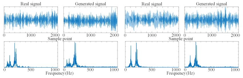
Sensors 2021, 21, 5494 4 of 22
enhancement effect of the method in Section 2. Section 4 describes the theory of MC1DCNN,
combines it with AMVMD and embeds the DCGAN module in the model to form a fault
diagnosis model under an unbalanced dataset. Section 5 applies the model of this paper
to the fault diagnosis of the rolling mill fault simulation test bench and gets good results.
Additionally, we compare this model with the approximate model and existing models to
prove the advantage of this model. Finally, the conclusion is drawn in Section 6.
2. AMVMD Signal Processing and Unbalanced Data Generation
2.1. Iterative Acceleration of MVMD
The MVMD algorithm has been recently proposed to solve the problem of cooperative
decomposition of multi-channel data and to solve the problem that VMD can only handle
single-channel signal. The multi-channel signal can excite the noise reduction ability of the
Wiener filter and improve the signal processing effect of MVMD. MVMD converts the IMF
component of the multi-channel signal into a set of AM-FM signals as u(t):
u(t) = uc (t) = ac (t) cos(φc (t)) (1)
where ac (t) is the amplitude of the c-th component and ϕc (t) is the phase of the
c-th component.
Taking the square of the L2 parametric of the mixed signal to find the u(t) bandwidth,
and then the constrained variational optimization of the u(t) bandwidth of the multi-
channel signal is performed. It is required to minimize the bandwidth sum of the individual
components separated in the c signals, while ensuring the accuracy of each classification,
modeled as follows.
K,c − jω t 2
min ∑ ∑ k∂t [u+ (t)e K ]k ,
{uK,c }{ωk } K c 2 (2)
∑ uK,c (t) = xc (t), c = 1, 2, 3, · · · , c
K
where K is the number of IMF, c is the number of channels of the input signal, and ω k is the
center frequency of each mode.
The constrained variational model is constructed by using the Lagrange multiplier
method and is transformed into an unconstrained variational problem by introducing the
penalty factor α with the Lagrange multiplier λ(t). Construct the Lagrange function model
as follows:
K,c
L({uK,c }, {ωK }, λc ) = α∑ ∑ k∂t [u+ (t)e− jωK t ]k
K c
2
(3)
+∑ k xc (t) − ∑ uK,c (t)k + ∑ λc (t), xc (t) − ∑ uK,c (t)
c K 2 c K
The alternating direction multiplier method is used to transform the optimization
problem into a suboptimization problem, and the optimal mode and center frequency of
the multivariate signal are obtained by iteratively updating the subproblem.
In this paper, to address the problem of the slow iterative search speed of MVMD, an
iterative operator is introduced to accelerate the solution process, and the specific iterative
process is as follows.
n o
(1) Initialize û1K,c , ωK1 ,λ̂1c , set n = 0, ε= 10−7 .
n on o
(2) Set n = n + 1, and execute a loop to update ûnK,c +1
, ωKn+1 and λ̂nc +1 until iterative
precision is reached.
λ̂c (ω )
x̂c − ∑i6=K ûi,c (ω ) + 2
+1
ûnK,c (ω ) = 2
(4)
1 + 2α(ω − ωK )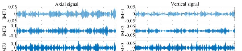
Sensors 2021, 21, 5494                                                                                                    5 of 22

                                                                               R∞                            2
                                                                          ∑        0       ω |ûK,c (ω )| dω
                                                                           c
                                                              ωKn+1   =            R∞                    2
                                                                                                                             (5)
                                                                            ∑          0   |ûK,c (ω )| dω
                                                                               c

                               Update λ̂nc +1 for all ω > 0
                                                                                           p
                                                                t n +1 = (1 +                  1 + 4tn 2 )/2                 (6)

                                                     λ̂cn+1 (ω ) = λ̂nc (ω ) + τ ( x̂c (ω ) − ∑ ûnK,c
                                                                                                    +1
                                                                                                       (ω ))                 (7)
                                                                                                             K

                                                                                       tn − 1
                                                 λ̂n+1 (ω ) = λ̂n+1 (ω ) + (                   )[λ̂n+1 (ω ) − λ̂n (ω )]      (8)
                                                                                        t n +1
                         (3)   Stop the iteration when the iteration accuracy is satisfied and output the set of modes
                               uK and the center frequency ω K .
                                                                                                     2
                                                                               +1
                                                                          kûnK,c − ûnK,c k2
                                                                ∑∑                 kûnK,c k22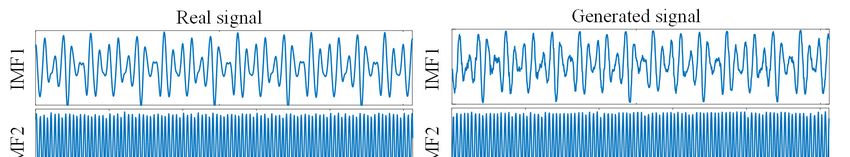
discriminator D, it is expected that when the input is G(z), D discriminates it as false, i.e.,
as D(G(z)) = 0. That is, for the problem of minimizing G and maximizing D, the discrimi-
nator and generator model loss functions are shown in (12) and (13).
Sensors 2021, 21, 5494 max V ( D, G ) = Ex − Pdata ( x ) [log( D( x))] + Ez − Pg ( z ) [log(1 − D(G( z )))] 6 of 22 (12)
D
min V ( D, G) = Ez − Pg ( z ) [log(1 − D(G ( z )))] (13)
G
minV ( D, G ) = Ez− Pg (z) [log(1 − D ( G (z)))] (13)
G
Through adversarial learning, the functions of G and D are continuously improved,
and Through
the finaladversarial
mathematical model
learning, isfunctions
the as follows.
of G and D are continuously improved,
and the final mathematical model is as follows.
min max V ( D, G ) = Ex − Pdata ( x ) [log D( x)] + Ez − Pg ( z ) [log(1 − D(G ( z )))] (14)
G D
min maxV ( D, G ) = Ex− Pdata ( x) [log D ( x )] + Ez− Pg (z) [log(1 − D ( G (z)))] (14)
G D
where x is the real sample; Pdata is the distribution of real data; and Pg is the distribution of
noise.x is the real sample; Pdata is the distribution of real data; and Pg is the distribution
where
of noise.
Radford proposed a DCGAN algorithm, which greatly improves the performance of
Radford proposed a DCGAN
GAN [30]. Additionally, algorithm,
in [36], Mirza whichthe
restricted greatly improves
generation the performance
process by inputting con-
of GAN [30]. Additionally, in [36], Mirza restricted the generation process by inputting
ditional variables to solve the problem that the training process is unstable with the gen-
conditional variables to solve the problem that the training process is unstable with the
eration results and the generated samples differ from the generation target, which in turn
generation results and the generated samples differ from the generation target, which
guides
in the generation
turn guides of theofdesired
the generation samples.
the desired In this
samples. paper,
In this DCGAN
paper, DCGAN is used to to
is used generate
the AMVMD reconstructed signal, and the generator mainly consists
generate the AMVMD reconstructed signal, and the generator mainly consists of four of four deconvolu-
tional layers and
deconvolutional the discriminator
layers mainlymainly
and the discriminator consists of four
consists of convolutional layers,
four convolutional as shown
layers,
as shown in Figure 1. The reconstructed signal removes the invalid features and retains faulty
in Figure 1. The reconstructed signal removes the invalid features and retains the
features,
the which can
faulty features, reduce
which canthe generation
reduce of invalid
the generation features
of invalid by DCGAN
features and improve
by DCGAN and the
improve
ability ofthe ability oftoDCGAN
DCGAN generate to virtual
generate virtual samples.
samples.
Figure1.1.The
Figure Thestructure
structure of DCGAN.
of DCGAN.
3. Analysis of Simulated Signals
3.1. Construction of Simulation Signal
The rolling mill multi-row rolling bearing vibration signal is a non-linear, non-stationary
modulated signal; according to the actual working conditions, we set the amplitude modu-
lation signal (x1 ), frequency modulation signal (x2 ), and harmonic signal (x3 ) to simulate
vibration signal. Each frequency of the simulated signals are as follows: f 1 = 80 Hz,
f 2 = 30 Hz, f 3 = 200 Hz, f 4 = 50 Hz, f 5 = 300 Hz, and the main characteristic frequencies are
f 1 , f 3 and f 5 .
x1 = cos(2π f 1 t)[1 + sin(2π f 2 t)]
x = sin[2π f 3 t + cos(2π f 4 t)] (15)
2
x3 = sin(2π f 5 t)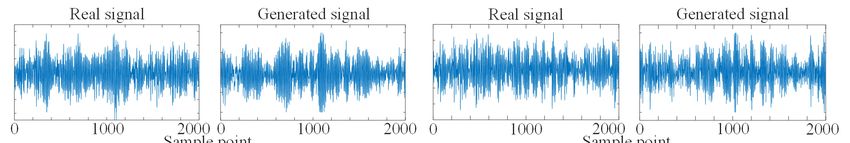
x1 = cos(2π f1t )[1 + sin(2π f 2t )]
x2 = sin[2π f3t + cos(2π f 4t )] (15)
x = sin(2π f t )
Sensors 2021, 21, 5494 3 5 7 of 22
In the actual signal acquisition, due to the complex transmission path and noise in-
terference, the sensor acquisition vibration signal is different, so we simulate each channel
signal with
In thedifferent weighting
actual signal ratiosdue
acquisition, for the three
to the simulated
complex signals as
transmission follows.
path and noise
interference, the sensor acquisition vibration signal is different, so we simulate each channel
signal with s1 = 0.45
different x1 + 0.85
weighting x2 +for
ratios 0.62 3 + nsimulated
thexthree 1 signals as follows.
s2 = 0.85 x1+ 0.7 x2 + 0.35
s1 = 0.45x
x3 +2 n+2 0.62x3 + n1
1 + 0.85x
(16)
s = 0.6 x + 0.4 + 0.91 +
x20.85x
s2 = + n23+ 0.35x3 + n2
x30.7x (16)
3 1
s3 = 0.6x1 + 0.4x2 + 0.9x3 + n3
where n1, n2, n3 and are 25db, 18db and 13db noise signals, respectively.
where n1 , n2 , n3 and are 25 db, 18 db and 13 db noise signals, respectively.
The
Thetime
timedomain
domain waveforms
waveforms and andfrequency
frequency domain
domain character
character ofthree-channel
of the the three-channel
simulated signal are shown in Figure
simulated signal are shown in Figure 2. 2.
Figure Time
Figure2. 2. domain
Time andand
domain frequency domain
frequency FigureFigure
domain of simulation signal. signal.
of simulation
3.2. Algorithm Performance Comparison
3.2. Algorithm Performance Comparison
We use MEMD, MVMD and AMVMD to decompose the simulated signal, set the
We use
number MEMD,
of modes MVMD
K of MVMDand to 4 AMVMD to decompose
and the penalty the simulated
factor α to 2000, and set thesignal,
K and αset the
number of modes
of AMVMD K of2434
to 4 and MVMD after to 4 and the by
optimization penalty factor α to 2000,
GA, respectively. andrequired
The time set the for
K and α
of MVMD
AMVMD andtoAMVMD
4 and 2434 after optimization
to process by GA,respectively.
signals of different The 10
lengths was calculated time required
times and for
averaged,
MVMD andand the results
AMVMD are shown
to process in Table
signals of1.different
The operating environment
lengths is Windows
was calculated 10, and
10 times
the CPU and
averaged, is Intel
thei7-9750H (2.60shown
results are GHz), and the RAM
in Table is 16operating
1. The GB. The AMVMD computation
environment is Windows
10,time
the is
CPUsignificantly reduced after
is Intel i7-9750H (2.60the introduction
GHz), and theofRAM the iterative operator.
is 16 GB. The AMVMD computa-
tion time is significantly reduced after the introduction of the iterative operator.
Table 1. Comparison of operation time.
Table
Length of 1. Comparison
Signal of operation
Computation time.
Time of MVMD(s) Calculation Time of AMVMD (s)
2000
Length of Signal Computation Time of0.737
MVMD(s) 0.506
Calculation Time of AMVMD (s)
4000 3.345 2.001
2000 6000 0.737 8.185 0.506
5.020
4000 8000 3.345 11.887 7.241
2.001
10,000 15.817 9.642
6000 12,000
8.185 22.567 5.020
14.037
14,000 30.682 19.367
16,000 41.052 26.477
Fourteen groups of IMFs are obtained by MEMD, and we only take the first five
groups of IMFs for frequency domain analysis, as shown in Figure 3a, the MVMD decom-
position results as shown in Figure 3b, and the AMVMD decomposition results as shown
in Figure 3c. It can be seen from Figure 3 that all three algorithms adaptively decompose
the multivariate simulation signal to obtain the IMF component of the response principal
frequency. However, some of the same frequency components are reflected in different
IMFs, i.e., the phenomenon of mode mixing appears. The most serious modal mixing is
found in the IMFs of MEMD, where IMF3 has a primary frequency of 150 Hz (f 3 − f 4 )
and IMF5 has a primary frequency of 50 Hz (f 2 − f 1 ); both frequencies are the sideband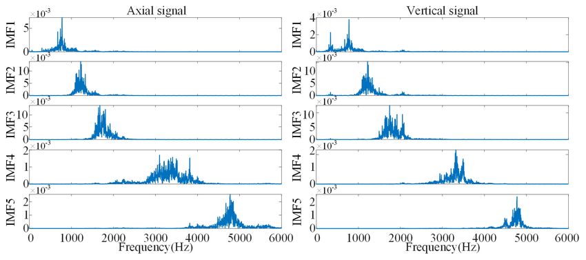
position results as shown in Figure 3b, and the AMVMD decomposition results as shown
in Figure 3c. It can be seen from Figure 3 that all three algorithms adaptively decompose
the multivariate simulation signal to obtain the IMF component of the response principal
frequency. However, some of the same frequency components are reflected in different
Sensors 2021, 21, 5494 8 of 22
IMFs, i.e., the phenomenon of mode mixing appears. The most serious modal mixing is
found in the IMFs of MEMD, where IMF3 has a primary frequency of 150 Hz (f3 − f4) and
IMF5 has a primary frequency of 50 Hz (f2 − f1); both frequencies are the sideband frequen-
cies of the primary
frequencies frequency
of the primary peak ofpeak
frequency the oforiginal signal.
the original Additionally,
signal. Additionally, therethere
are more
are
cluttered noise frequencies
more cluttered in the IMFs
noise frequencies in theofIMFs
MEMD, while the
of MEMD, IMFs
while theofIMFs
MVMD and AMVMD
of MVMD and
are basically
AMVMD arefree of noise
basically freefrequencies.
of noise frequencies.
In
In Figure 3b,c,the
Figure 3b,c, theIMFs
IMFsare arewell
well decomposed
decomposed according
according to major
to the the major center center frequen-
frequencies,
and the corresponding side bands appear on both sides of the
cies, and the corresponding side bands appear on both sides of the major center frequen- major center frequencies,
and and
cies, the the
sideside
band frequencies
band frequencies in in
IMF1IMF1 areare5050Hz Hzand and110 110Hz Hz (f(f11 ±±f2),f 2and
), and
thethe
sideside
band
band frequencies
frequencies in IMF2 in are
IMF2 150areHz150 andHz250andHz250
(f3 ±Hz 3 ± there
f4),(fand f 4 ), and there is basically
is basically no main no main
frequency
frequency
peak peak
in IMF4, andin the
IMF4, andisthe
signal signal
well is well decomposed.
decomposed. However, aHowever, left side band a leftfrequency
side band of
frequency of 250 Hz (f 3 + f
250 Hz (f3 + f4) appears in IMF3, and the overall peak of the side band frequencyband
4 ) appears in IMF3, and the overall peak of the side of the
frequency
modal of the
mixing inmodal
IMF3 of mixing
AMVMD in IMF3 of AMVMD
is reduced is reduced
compared compared
to that of MVMD. to that of MVMD.
(a) MEMD.
Sensors 2021, 21, x FOR PEER REVIEW 9 of 23
(b) MVMD.
(c) AMVMD.
Figure 3. Effect comparison of three methods.
Figure 3. Effect comparison of three methods.
3.3. Generation of Simulation Data
We use DCGAN to generate the IMFs of the simulated signal; the training set is the
IMF1–IMF3 of the three-channel simulated signal, and the sample length is set to 1024.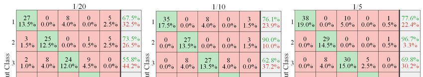
(c) AMVMD.
Sensors 2021, 21, 5494                                                                                                 9 of 22
                                    Figure 3. Effect comparison of three methods.

                         3.3.3.3.
                               Generation  of Simulation Data
                                  Generation of Simulation Data
                               WeWeuse
                                     useDCGAN
                                         DCGAN to   to generate  theIMFs
                                                       generate the   IMFsofof
                                                                             thethe  simulated
                                                                                  simulated      signal;
                                                                                             signal;      the training
                                                                                                     the training  set is set
                                                                                                                          the is the
                         IMF1–IMF3     of the  three-channel     simulated   signal,   and  the sample    length
                           IMF1–IMF3 of the three-channel simulated signal, and the sample length is set to 1024.  is set  to 1024.
                         The
                           Thetime-domain
                                 time-domainwaveform
                                               waveform comparison
                                                            comparison andand frequency-domain
                                                                               frequency-domain       character
                                                                                                    character     comparison of
                                                                                                                comparison
                         the generated signal and the real signal for each channel are shown Figure4.4. The
                           of  the generated  signal  and  the real signal for each  channel  are shown    in Figure      The gen-
                           generated
                         erated  signalsignal well simulates
                                        well simulates          the time-domain
                                                          the time-domain           waveform
                                                                               waveform        characters
                                                                                           characters  andand    frequency-
                                                                                                              frequency-domain
                           domain characters
                         characters  of the realofsignal,
                                                   the realwhich
                                                            signal,can
                                                                    which  can realize
                                                                       realize         the supplement
                                                                                the supplement          of scarce
                                                                                                   of scarce       data.
                                                                                                                data.

                                             (a) Time domain waveform.

                                           (b) Frequency domain character.
                                Figure 4. Comparison of real signal and generated signal.
                             Figure 4. Comparison of real signal and generated signal.
                           4. Fault Diagnosis Model Based on AMVMD-MC1DCNN
                           4.1. One-Dimension Convolutional Neural Network
                                 CNN was originally applied to image recognition techniques [37]. The local connec-
                           tivity, weight sharing, and down-sampling character of CNN make the network structure
                           massively reduced, and CNN can make full use of the local features of the data itself and
                           thus improve the computational efficiency. The structure of CNN includes convolutional
                           layers, a pooling layer, a fully connected layer and an output layer [38]. The main difference
                           between 1DCNN and CNN is that the input dimension of the character is one-dimensional,
                           so 1DCNN consists of one-dimensional convolutional layers, one-dimensional pooling
                           layers, a fully connected layer and a Softmax classifier, and the structure of 1DCNN is
                           shown in Figure 5.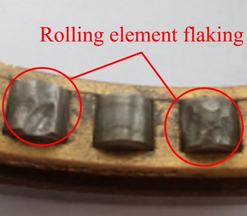
massively reduced, and CNN can make full use of the local features of the data itself and
thus improve the computational efficiency. The structure of CNN includes convolutional
layers, a pooling layer, a fully connected layer and an output layer [38]. The main differ-
ence between 1DCNN and CNN is that the input dimension of the character is one-di-
Sensors 2021, 21, 5494 mensional, so 1DCNN consists of one-dimensional convolutional layers, one-dimensional
10 of 22
pooling layers, a fully connected layer and a Softmax classifier, and the structure of
1DCNN is shown in Figure 5.
.
Figure5.5.One-dimension
Figure One-dimensionconvolutional neural
convolutional network.
neural network.
Assuming that a one-dimensional signal xi is the output of layer i, its convolution is
Assuming that a one-dimensional signal xi is the output of layer i, its convolution is
computed in the following way.
computed in the following way.
x lj = f ( xxj il=−1 ∗f (w
l
∑l +xibl )∗ wij + bj )
l −1 l l
(17)
i ∈ijN j
j (17)
i∈N j
where Nj is the j-th convolutional region of the l-1st layer; x lj is the j-th input to the
where Nj is of
convolution thel j-th
layer;convolutional region
w is the weight of the
matrix (convolution xlj is the
l-1st layer; kernel); b isj-th
theinput to the
bias of the con-
convolution
volution of layer; f iswthe
l layer; nonlinear
is the weightactivation function. kernel); b is the bias of the convo-
matrix (convolution
lution layer; f is the nonlinear activation function.as the down-sampling layer, reduces
The one-dimensional pooling layer, also known
the dimensionality of the convolutional features and reduces the computational effort of
The one-dimensional pooling layer, also known as the down-sampling layer, reduces
the classifier. The maximum pooling process is usually chosen to ensure the invariance of
the dimensionality of the convolutional features and reduces the computational effort of
feature scales and reduce the size of the input data.
the classifier. The maximum pooling process is usually chosen to ensure the invariance of
feature scales and reduce the size
x l =off (the input
down ( x l −1data.
+ bl )) (18)
j j j
l l −1 l
where down() is x = function.
sampling
j f (down( x + b )) j j (18)
The fully connected layer can rearrange the characters extracted from the previous
where down()layers
convolutional is sampling function.
and pooling layers into a column, and the Dropout function is usually
added to suppress overfitting andcan
The fully connected layer rearrange
improve the characters
generalization abilityextracted
of CNN. from the previous
convolutional layers and pooling layers into a column, and the Dropout function is usu-
= fimprove
ally added to suppress overfittingδiand (wi pi + bgeneralization
i) ability of CNN. (19)
δ ithe
where i = 1, 2, · · · , k, δi is = i-th i pi + bi )
f (woutput, and k in total. (19)
The most commonly used classifier for CNN is the supervised learning Softmax
where i =
classifier. 1, 2, , k , δthe
Additionally, i network
is the i-thisoutput,
optimally
andtrained using the Adam optimization
k in total.
algorithm, whichcommonly
The most in turn accomplishes the multi-classification
used classifier task. The output
for CNN is the supervised of Softmax
learning Softmax clas-
can be viewed as a probability problem.
sifier. Additionally, the network is optimally trained using the Adam optimization algo-
rithm, which in turn accomplishes the multi-classification
eδi task. The output of Softmax can
be viewed as a probability problem. p ( i ) = K
(20)
∑ eδk
k =1
where p(i) is the probability of each output, the sum of p(i) is 1, and K is the number
of categories.
4.2. Multi-Channel One-Dimension Convolutional Neural Network
In this paper, a multi-channel one-dimensional convolutional fusion layer is added to
1DCNN, as shown in Figure 6. M1DCNN can be used for multi-channel signal processing,
which can synthetically consider multiple directional vibration signals for fault diagnosiscategories.
4.2. Multi-Channel One-Dimension Convolutional Neural Network
In this paper, a multi-channel one-dimensional convolutional fusion layer is added
Sensors 2021, 21, 5494 11 of 22
to 1DCNN, as shown in Figure 6. M1DCNN can be used for multi-channel signal pro-
cessing, which can synthetically consider multiple directional vibration signals for fault
diagnosis analysis, and AMVMD reconstructed signal can further reduce noise interfer-
analysis,
ence andand AMVMD
highlight reconstructed
fault signal
characters by can furtherone-dimensional
multi-channel reduce noise interference and pro-
convolution
highlight
cessing. fault characters by multi-channel one-dimensional convolution processing.
Figure6.6.Multi-channel
Figure Multi-channelone-dimension
one-dimension convolutional
convolutional fusion.
fusion.
When
Whenthetheinput
inputtotothe
theconvolution
convolutionlayer is aismulti-channel
layer signal,
a multi-channel a multi-channel
signal, a multi-channel
convolution kernel is used for the operation, and a one-dimensional convolution
convolution kernel is used for the operation, and a one-dimensional convolution operation
opera-
is performed in each channel individually. In order to add the correlation of the respective
tion is performed in each channel individually. In order to add the correlation of the re-
channels, we need to compute the weighted summation of each channel at the same
spective channels, we need to compute the weighted summation of each channel at the
position to obtain the 1D convolutional output at that position.
same position to obtain the 1D convolutional output at that position.
m k
m k
xl = ∑l −1f j ( ∑l −(1xij ×l −w
l −1 l −1 l −1
x = f j ( ( jx=ij1 ×iw 1 ij ) + bij )
l (21)
=1ij
) + bij ) (21)
j =1 i =1
where x l is the output of the l-th convolutional layer; xijl −1 is the
l −1 i-th character input of the
l
where x is the output of the l-th convolutional layer; x is the i-th character input of
ij l −1 is the i-th convolutional
l-1st convolutional layer of channel j, with k character inputs; w ij
l −1
the l-1st
kernel convolutional
of the l-1st layer oflayer
channel j; bijl −1 is j,the
of channel with k character
ith bias the l-1st w
value ofinputs; layer is channel
ij of the i-th j;convo-
f
is the nonlinear activation function; m is the number l −1 of channels.
lutional
The kernel of the l-1st
multi-channel layer of channel
one-dimensional j; bij isfusion
convolutional the ithlayer
bias can
value of the l-1st
effectively layer of
realize
the fusionj;and
channel f is character extraction
the nonlinear of multi-channel
activation function; m signals.
is the The pooling
number layer of M1DCNN
of channels.
also uses
The maximum
multi-channelpooling, followed by a convolutional
one-dimensional fully connectedfusion
layer and
layera Softmax classifier.
can effectively realize
the fusion and character extraction of multi-channel signals. The pooling layer of
4.3. Fault Diagnosis Model
M1DCNN also uses maximum pooling, followed by a fully connected layer and a Softmax
The fault diagnosis model based on AMVMD-M1DCNN proposed in this paper
classifier.
is shown in Figure 7, which consists of a multichannel input layer, multivariate mode
variational reconstruction, conditional deep convolutional generation adversarial network,
4.3. Fault Diagnosis Model
1D convolutional, 1D pooling, and fully connected and Softmax classifiers.
The fault diagnosis
Considering model
the rich fault based oninAMVMD-M1DCNN
information proposed
the axial vibration signal of the in this mill
rolling paper is
multi-row bearings, and the low signal-to-noise ratio of the vertical vibration signals, themode
shown in Figure 7, which consists of a multichannel input layer, multivariate
axial and vertical vibration signals are input into the fault diagnosis model simultaneously.
The input signal is a two-channel one-dimensional signal of 1 × 2048 × 2. The model
consists of two parts: offline training and online detection. The existing label data is used
to train the fault diagnosis model, and the model is used to classify the collected data.
Embedding DCGAN can improve the diagnosis accuracy of fault diagnosis model under
the condition of unbalanced training datasets. After each channel signal is reconstructed
by AMVMD, it is input into M1DCNN for individual convolution calculation, and the
multi-channel can more comprehensively explore the information of fault vibration signal
characters than the single channel.to train the fault diagnosis model, and the model is used to classify the collected data.
Embedding DCGAN can improve the diagnosis accuracy of fault diagnosis model under
the condition of unbalanced training datasets. After each channel signal is reconstructed
by AMVMD, it is input into M1DCNN for individual convolution calculation, and the
Sensors 2021, 21, 5494 12 of 22
multi-channel can more comprehensively explore the information of fault vibration signal
characters than the single channel.
Fault Diagnosis Model.
Figure 7.Model.
Figure 7. Fault Diagnosis
5.5.Experiments
Experimentsand
andResults
Results Analysis
Analysis
ToToverify
verifythe
theeffectiveness
effectiveness of
of the
the diagnostic
diagnosticmodel,
model,ananexperimental
experimentalrolling mill
rolling fault
mill fault
simulation test bench was used for bearing vibration signal acquisition, and the test bench
simulation test bench was used for bearing vibration signal acquisition, and the test bench
is shown in Figure 8. The parameters of the rolling mill are as follows: the diameter of the
is shown in Figure 8. The parameters of the rolling mill are as follows: the diameter of the
roll is 120 mm, the length of the roll is 90 mm, the speed of the main motor is 180 r/min,
roll is 120 mm, the length of the roll is 90 mm, the speed of the main motor is 180 r/min,
the maximum rolling force is 12 tons; the vibration sensor is YS8202, the acceleration
the maximum
sensor, rollingsensor
and pressure force is 12 tons;
model the vibration
is HZC-01, and thesensor is YS8202,
sampling theisacceleration
frequency 2000 Hz. The sen-
sor,
Sensors 2021, 21, x FOR PEER REVIEW and pressure sensor model is HZC-01, and the sampling frequency is 2000
experimental bearings are double-row cylindrical roller bearings, and the bearing type of 23Hz.13The
experimental
is NU1012. bearings are double-row cylindrical roller bearings, and the bearing type is
NU1012.
Figure8.8.Experimental
Figure Experimentalrolling
rolling mill
mill bearing
bearing fault
fault diagnosis
diagnosis testtest bench.
bench.
We
Wecollected
collectedvibration
vibrationdata
datafrom thethe
from operating
operatingsideside
of the rolling
of the mill mill
rolling and and
selected
selected
bearings
bearingswith
withrolling
rollingelement
element scratches, bearings
scratches, bearingswith broken
with cages,
broken bearings
cages, withwith
bearings rolling
rolling
element flaking, bearings with mixed faults (rolling element flaking and broken
element flaking, bearings with mixed faults (rolling element flaking and broken cage) andcage) and
normal
normalbearings
bearingsfor fault
for data
fault collection;
data the the
collection; labels of the
labels offive
thetypes of bearings
five types were set
of bearings to set
were
1–5 in order. The bearing failure is shown in Figure 9. In each experiment, we performed
to 1–5 in order. The bearing failure is shown in Figure 9. In each experiment, we performed
two passes of the rolling process, and we collected 120,000 data points each time, for a total
two passes of the rolling process, and we collected 120,000 data points each time, for a
total of 480,000 data points in two experiments. The data are divided according to a sam-
ple length of 2048, with 240 samples available for each bearing.We collected vibration data from the operating side of the rolling mill and selected
bearings with rolling element scratches, bearings with broken cages, bearings with rolling
element flaking, bearings with mixed faults (rolling element flaking and broken cage) and
Sensors 2021, 21, 5494 13 of 22
normal bearings for fault data collection; the labels of the five types of bearings were set
to 1–5 in order. The bearing failure is shown in Figure 9. In each experiment, we performed
two passes of the rolling process, and we collected 120,000 data points each time, for a
totalofof 480,000
480,000 data
data points
points in two
in two experiments.
experiments. The data
The data are divided
are divided according
according to a sam-
to a sample
length of 2048, with 240 samples available for each bearing.
ple length of 2048, with 240 samples available for each bearing.
(a) Normal bearing (b) Rolling element scratch
(c) Broken cage (d) Rolling element flaking
Figure 9. Four
Figure kinds
9. Four ofof
kinds test
testbearing.
bearing.
5.1.5.1. Signal
Signal Processing
Processing bybyAMVMD
AMVMD
WeWe used
used thetheAMVMD
AMVMD to to decompose
decompose vertical
verticalvibration
vibrationsignals andand
signals axialaxial
vibration
vibration
signals and then chose the better IMFs to reconstruct the signal. AMVMD had reduced
signals and then chose the better IMFs to reconstruct the signal. AMVMD had reduced
the effect of the number of IMFs K on the decomposition effect; if K is set too large, the
the effective
effect offault
the number of IMFs
characteristics willKbeon the decomposition
stripped effect;
to the worse IMFs, so if
weKsetis K
set∈ too
[3,6]large,
and the
effective fault characteristics
α ∈ [500,4000] and used thewill
GAbeto stripped to the worse
find the optimal we set K ∈in [3,6]
IMFs, so parameters
decomposition this and
α ∈ [500,4000] and used the GA to find the optimal decomposition parameters
range. The parameters of GA were set as follows: the population size is 10, the number in this
range. The parameters
of population of GA
evolution were
is 25, the set as follows:
probability the population
of crossover sizethe
is 0.8 and is 10, the number
probability of of
variation evolution
population is 0.1. We recorded the best
is 25, the fitness and
probability of the fitness average
crossover is 0.8 of
andall individuals
the probability for of
each evolution. The iterative search curves for the four fault signals are shown in Figure 10,
and the decomposition parameters are shown in Table 2.
Table 2. Optimized parameters for four types of fault signals.
Types of Faults Number of IMF Penalty Factor α
Rolling element scratch 5 2658
Broken cage 6 2941
Rolling element flaking 5 2931
Mixed faults 6 2137
The decomposition results of bearings with rolling body flaking are shown in Figure 11;
the periodic waveform can be initially seen from the time domain of IMF1, IMF2 and IMF3,
while the time domain waveforms of IMF4 and IMF5 are more chaotic. The frequency
domain feature maps of the five IMFs appear with slight modal mixing, but the central
frequencies of the individual IMFs are well separated.Sensors 2021, 21, x FOR PEER REVIEW 14 of 23
Sensors 2021, 21, 5494 14 of 22
variation is 0.1. We recorded the best fitness and the fitness average of all individuals for
each evolution. The iterative search curves for the four fault signals are shown in Figure
10, and the decomposition parameters are shown in Table 2.
(a) Rolling element scratch (b) Broken cage
Sensors 2021, 21, x FOR PEER(c) Rolling
REVIEW element flaking (d) Mixed fault 15 of
Figureof10.
Figure 10. Optimization curve GA.Optimization curve of GA.
Table 2. Optimized parameters for four types of fault signals.
Types of Faults Number of IMF Penalty Factor α
Rolling element scratch 5 2658
Broken cage 6 2941
Rolling element flaking 5 2931
Mixed faults 6 2137
The decomposition results of bearings with rolling body flaking are shown in Figure
11; the periodic waveform can be initially seen from the time domain of IMF1, IMF2 and
IMF3, while the time domain waveforms of IMF4 and IMF5 are more chaotic. The fre-
quency domain feature maps of the five IMFs appear with slight modal mixing, but the
central frequencies of the individual IMFs are well separated.
(a) Time domain waveform diagram
(b) Frequency domain feature map
Figure 11. Figure 11. Decomposition
Decomposition results of results
bearingsof with
bearings withelement
rolling rolling flaking.
element flaking.
We used the WPE as the evaluation index; the WPE of each IMF for eight kinds
signals are shown in Figure 12. It can be found that the WPE of the first two IMFs a
significantly smaller than the other IMFs, which coincides with the regularity of the tim
domain waveform, and the signal period regularity is the strongest. It can be considereSensors 2021, 21, x FOR PEER REVIEW 16 of 24
Sensors 2021, 21, 5494 15 of 22
Figure 11. Decomposition results of bearings with rolling element flaking.
We used
We used the
the WPE
WPE as as the
the evaluation
evaluation index;
index; the
the WPE
WPE of of each
each IMF
IMF for
for eight
eight kinds
kinds of
of
signals are shown in Figure 12. It can be found that the WPE of the first
signals are shown in Figure 12. It can be found that the WPE of the first two IMFs are two IMFs are
significantly smaller
significantly smaller than
than the
the other
other IMFs,
IMFs, which
which coincides
coincides with
with the
the regularity
regularity of of the
the time
time
domain waveform, and the signal period regularity is the strongest. It can
domain waveform, and the signal period regularity is the strongest. It can be consideredbe considered
that IMF1
that IMF1 and
andIMF2
IMF2contain
containrich fault
rich character
fault information,
character information,so IMF1 and and
so IMF1 IMF2IMF2
are selected
are se-
to reconstruct
lected the axial
to reconstruct thevibration signal and
axial vibration vertical
signal vibration
and vertical signal. signal.
vibration
Sensors 2021, 21, x FOR PEER REVIEW 16 o
Figure 12. WPE of IMF of various signal.
5.2. Generate5.2.
Reconstructed Data by DCGAN
Generate Reconstructed Data by DCGAN
The sample Thedatasample
length ofdata length signal
the faulty of the and normal
faulty signalsignal was set to
and normal 2048,was
signal andset
theto 2048, a
training set of DCGAN was composed according to the unbalanced ratio of 1/10
the training set of DCGAN was composed according to the unbalanced ratio (200 sets of of 1/10 (
normal bearing data samples and 20 sets of each fault samples), and we input the condition
sets of normal bearing data samples and 20 sets of each fault samples), and we input
variables at condition
the same time to generate
variables the faulty
at the same time bearing reconstruction
to generate signal under
the faulty bearing the
reconstruction sig
unbalanced condition. The time domain waveforms and frequency domain characters of
under the unbalanced condition. The time domain waveforms and frequency dom
the real and generated signals are shown in Figure 13. It can be seen that the time domain
characters of the real and generated signals are shown in Figure 13. It can be seen that
waveforms of the real signal and the generated signal are similar, and the main frequency
time domain waveforms of the real signal and the generated signal are similar, and
characteristics of the frequency domain maps are basically the same, and we can consider
main frequency characteristics of the frequency domain maps are basically the same, a
that the reconstructed signal generated by DCGAN has better fault characteristics. We
we can consider that the reconstructed signal generated by DCGAN has better fault ch
combined the generated data as supplementary samples with real samples into a balanced
acteristics. We combined the generated data as supplementary samples with real samp
dataset to train the fault diagnosis model and improve the accuracy of the diagnosis model
into a balanced dataset to train the fault diagnosis model and improve the accuracy of
under unbalanced sample conditions.
diagnosis model under unbalanced sample conditions.
(a) Rolling element scratch
Figure 13. Cont.Sensors 2021, 21, 5494 16 of 22
(a) Rolling element scratch
(b) Broken cage
Sensors 2021, 21, x FOR PEER REVIEW 17
(c) Rolling element flaking
(d) Mixed faults
Figure 13.Figure
Comparison of time domain
13. Comparison waveforms
of time domain and frequency
waveforms anddomain features
frequency of real
domain and generated
features signals.
of real and
generated signals.
5.3. Fault Diagnosis by MC1DCNN
5.3. Fault Diagnosis by network
The MC1DCNN structure of MC1DCNN is shown in Table 3. In the first layer, we u
The network
a widestructure of MC1DCNN
convolutional kernel to is shownfilter
further in Table 3. In
out the the first layer,
interference we used
of noise and save the
a wide convolutional kernel to further filter out the interference of noise and save
culation time, and the subsequent convolutional kernels use smaller convolutional the ker
calculation time, and
to fully the subsequent
explore convolutional
the fault characters of the kernels
vibrationuse smaller convolutional
signal.
kernels to fully explore the fault characters of the vibration signal.
Table 3. Network structure of MC1DCNN.
Table 3. Network structure of MC1DCNN.
Network Convolution Input Output Activatio
Step
Network Structure Convolution KernelStructure Kernel OutputChannel
Input Channel Channel ChannelActivation Function
Step Functio
Convolutional layer 1 32 × 1 Convolutional2 32 2 Tanh
32 × 1 2 32 2 Tanh
Convolutional layer 2 4×1 layer 1 32 64 2 ReLU
Convolutional layer 3 4×1 Convolutional64 128 2 ReLU
Convolutional layer 4 4×1 128 4×1 128 32 2 64 ReLU2 ReLU
layer 2
Convolutional
All convolutional 4×1 64 128 2 ReLU
layer 3layers are edge-processed with the SAME function. Each convolu-
tion layer is followed by a pooling layer, and we used maximum pooling with a pooling
Convolutional
strip width of 2. The last pooling 4 ×layer
1 is connected
128 to the fully
128connected layer,
2 which ReLU
layer 4
has 1024 neurons. In order to suppress the overfitting phenomenon and improve the
All convolutional layers are edge-processed with the SAME function. Each conv
tion layer is followed by a pooling layer, and we used maximum pooling with a poo
strip width of 2. The last pooling layer is connected to the fully connected layer, w
has 1024 neurons. In order to suppress the overfitting phenomenon and improve the g
eralization ability of the model, we added the dropout function; finally, the Softmax cSensors 2021, 21, 5494 17 of 22
generalization ability of the model, we added the dropout function; finally, the Softmax
classifier is used for classification.
We performed fault diagnosis analysis on the training set under three unbalanced
ratios (1/20, 1/10, 1/5). We randomly selected 40 sets of various bearing data as the test
set, and the remaining 200 sets of normal bearing data and the corresponding proportional
quantities (10, 20, and 40) of four types of faulty bearing data as the training set. Addition-
ally, the confusion matrix of the diagnostic results of the model under the three ratios is
shown in Figure 14a. Under the condition of a lack of fault training data, the diagnosis
accuracy of the model is low, and with the increased ratio of fault data to normal data, the
diagnosis accuracy of the model improves.
We trained DCGAN using three unbalanced datasets and supplemented the unbal-
anced dataset with the data generated by DCGAN. Finally, MC1DCNN was trained with
the supplemented dataset, and we obtained three balanced ratio data diagnosis models,
and used the three models to identify and classify the test sets. The confusion matrix of
the classification results of the three models is shown in Figure 14b. After embedding the
Sensors 2021, 21, x FOR PEER REVIEW 18 of 23
DCGAN data supplementation module in the fault diagnosis model, the network diagnosis
accuracy under the three unbalanced data conditions was significantly improved, and the
diagnosis accuracy reaches more than 90% in all cases. DCGAN can effectively improve
improve the fault diagnosis
the fault diagnosis capabilitycapability of the
of the model model
in this in this
paper paper
under under unbalanced
unbalanced data
data conditions.
conditions.
(a) Classification results of unbalanced training set
(b) Classification results of DCGAN supplemental training set
Figure
Figure 14.
14. Confusion
Confusion matrix
matrix for
for different
different diagnosis
diagnosis models.
models.
The
The diagnostic
diagnostic results
results for
for the
the original
original signal
signal (OS)
(OS) input,
input, the MEMD reconstructed
the MEMD reconstructed
signal
signal input,
input, the
the AMVMD
AMVMD reconstructed
reconstructed signal
signal input
input and
and the
the combination
combination of
of the
the three
three
inputs
inputs with
with DCGAN
DCGAN areare shown
shown inin Figure
Figure 15.
15. AMVMD
AMVMD has has the
the highest
highest diagnosis
diagnosis accuracy
accuracy
under all types of ratio training sets, and when the unbalance ratio is 1/5, the model diag-
nosis accuracy is almost the same as the balanced data after combining AMVMD with
DCGAN, which further verifies the superiority of the fault diagnosis model proposed in
this paper.Sensors 2021, 21, 5494 18 of 22
under all types of ratio training sets, and when the unbalance ratio is 1/5, the model
diagnosis accuracy is almost the same as the balanced data after combining AMVMD with
DCGAN, which further verifies the superiority of the fault diagnosis model proposed
Sensors 2021, 21, x FOR PEER REVIEW in23
19 of
this paper.
Figure 15. Diagnosis
Figure accuracy
15. Diagnosis of various
accuracy models
of various underunder
models four scaled training
four scaled sets. sets.
training
5.4.Comparison
5.4. ComparisonExperiments
Experiments
ToTo furtherverify
further verifythe thesuperiority
superiorityofofthe thediagnosis
diagnosismodels
modelsininthisthispaper,
paper,we we combined
combined
threeprocessed
three processedsignals
signals(original
(original signal, MEMDMEMDreconstructed
reconstructedsignalsignaland
andAMVMD
AMVMD recon-
re-
structed signal) with three classification algorithms (DBN, 1DCNN,
constructed signal) with three classification algorithms (DBN, 1DCNN, MC1DCNN). We MC1DCNN). We ran-
domly selected
randomly selected 200200setssets
of data from
of data eacheach
from typetype
of bearing as the
of bearing astraining sets and
the training setsthe
andre-
the remaining
maining 40 sets40 of
sets of data
data as theastest
the sets
test and
sets calculated
and calculated the average
the average accuracy
accuracy of theofmodel
the
model
for 10for 10 diagnoses
diagnoses as shown as shown in Table
in Table 4. DBN, 4. DBN,
1DCNN 1DCNN selected
selected three three
modes modes of input
of input (single
(single
channel channel
verticalvertical
signalsignal
input,input,
singlesingle
channel channel
axial axial
signalsignal
inputinput and dual
and dual channel
channel signal
signal
mixing mixing
input). input). The implied
The implied layerlayer
number number
of DBNof DBN wastoset
was set 3. to 3. 1DCNN
1DCNN layerlayer struc-is
structure
ture
the is the as
same same as MC1DCNN
MC1DCNN aspossible.
as far as far as possible.
From TableFrom4, Table
it can 4,beitseen
can that
be seen that the
the AMVMD-
AMVMD-MC1DCNN model proposed in this paper has
MC1DCNN model proposed in this paper has the highest diagnosis accuracy. the highest diagnosis accuracy.
In order to verify the advantages of the AMVMD-MC1DCNN fault diagnosis model
in this
Tablepaper compared
4. Diagnosis with of
accuracy the existing
various faultmodels,
diagnosisthemodels.
existing approximate models were
selected to reproduce the results for comparison. A more comprehensive comparison
between 1DCNNInput Signal and MC1DCNNClassificationhas been made Model
in the results of this Accuracy
paper, so the
1DCNN model of the literature [25,26] is not compared subsequently. The 81.4%
Original signal (Vertical) DBN models selected
Original signal
for comparison are the(Axial)
VMD-ELM model of DBNthe literature [15], the MVMD-SVM 84.2% model
of theOriginal
literaturesignal
[17],(Mixed)
and the VMD-CNN DBN model of the literature [22]. 89.8% Since both the
Originalmodel
VMD-ELM signaland(Vertical)
the MVMD-SVM model 1DCNN require feature extraction84.3% of the vibration
signal, in the process
Original of performing MWPE
signal (Axial) 1DCNNfeature extraction, we found87.4% that the larger
embedding
Originaldimension
signal (Mixed) and scale factor of 1DCNNthe Multiscale Weighted Permutation 91.7% Entropy
(MWPE)
MEMDalgorithm
reconstructed increase
signalthe computing time significantly, so the CNN model has an
absolute advantage
(Vertical) in diagnostic time afterDBN training is completed. Therefore, 87.3%we ignore
theMEMD
time required for feature
reconstructed signal extraction and compare only the diagnostic accuracy of the
DBN 89.5%
(Axial)
MEMD reconstructed signal
DBN 91.6%
(Mixed)
MEMD reconstructed signal
1DCNN 87.5%
(Vertical)You can also read