EROSITA All-Sky Survey 1: Study of the Canis Major Dwarf Spheroidal Galaxy - Black ...
←
→
Page content transcription
If your browser does not render page correctly, please read the page content below
eROSITA All-Sky Survey 1:
Study of the Canis Major Dwarf Spheroidal Galaxy

             Bachelorarbeit aus der Physik

                      Vorgelegt von
                   Theresa Heindl
                    12. April 2021

                Dr. Karl Remeis-Sternwarte
    Friedrich-Alexander-Universität Erlangen-Nürnberg

          Betreuerin: Prof. Dr. Manami Sasaki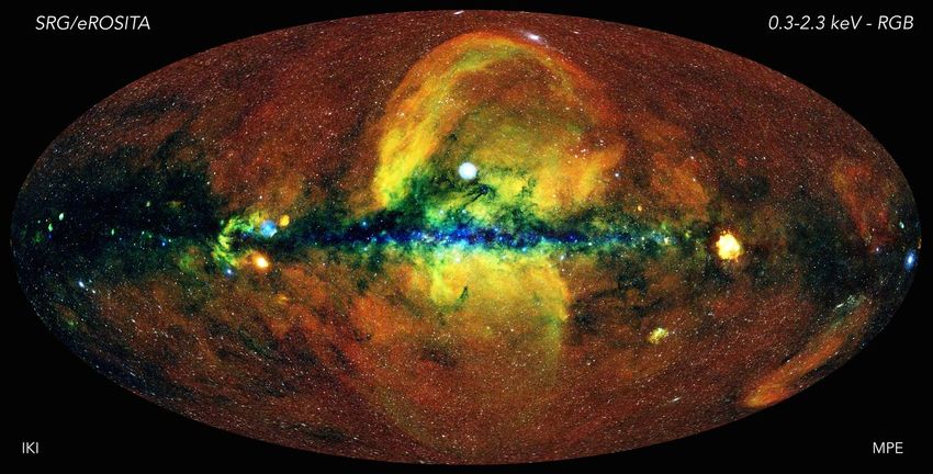
Abstract

   This work is a population study of the Canis Major Dwarf Spheroidal Galaxy
which is believed to be a dwarf satellite galaxy to the Milky Way. It is located close
to the galactic plane at (l, b) = (240◦ , -8◦ ). The aim of this thesis was to identify
possible Canis Major sources in eROSITA data. X-ray data of the eROSITA All-
Sky Survey 1 was studied and analysed by looking at the X-ray properties of the 17
676 detected sources and by calculating hardness ratios and the X-ray-to-optical
flux ratio. This analysis resulted in the conclusion that the eROSITA standard
bands are not useful for hardness-ratio based analysis and need to be adjusted for
better comparability.
   The observed X-ray sources were cross-matched with four other multiwavelength
catalogues in order to determine the class of sources: the optical Gaia and Skymap-
per catalogues, and the (near) infrared 2MASS and WISE catalogues. Through
criteria by Wright et al. (2010), background object candidates, foreground star
and elliptical galaxy candidates as well as normal galaxy candidates were identi-
fied with WISE data. By analysing colour-magnitude diagrams of Gaia matches
and theoretical isochrones, more galactic foreground and distant background can-
didates were excluded. A criterion based on the work of Martin et al. (2004)
identified a selection of Canis Major candidates on the red giant branch in 2MASS
magnitudes. Hardness ratio models suggest that most candidates have thermal
emission with low temperature and low absorption. Applying all criteria, 1289
final Canis Major candidates were identified and should be further discussed in
future studies.
Contents
   List of Tables . . . . . . . . . . . . . . . . . . . . . . . . . . . . . . . . . III
   List of Figures . . . . . . . . . . . . . . . . . . . . . . . . . . . . . . . . . IV

1 Introduction                                                                                                  1

2 Background Information                                                                                         2
  2.1 Stellar Evolution . . . . . . . . . . . . . . . . . . . . . . . . . . . .                                  2
  2.2 eROSITA Mission and X-Ray Sources . . . . . . . . . . . . . . . . .                                        4

3 Data Analysis                                                                                                  7
  3.1 eROSITA Catalogue . . . . . . . . . . . .         .   .   .   .   .   .   .   .   .   .   .   .   .   .    7
      3.1.1 Catalogue Contents . . . . . . . . .        .   .   .   .   .   .   .   .   .   .   .   .   .   .    7
      3.1.2 X-Ray Hardness Ratios . . . . . . .         .   .   .   .   .   .   .   .   .   .   .   .   .   .    8
  3.2 Multiwavelength Catalogues . . . . . . . .        .   .   .   .   .   .   .   .   .   .   .   .   .   .    9
      3.2.1 WISE Classification . . . . . . . . .       .   .   .   .   .   .   .   .   .   .   .   .   .   .   10
      3.2.2 Counterparts in the Gaia Catalogue          .   .   .   .   .   .   .   .   .   .   .   .   .   .   16
      3.2.3 Isochrones . . . . . . . . . . . . . .      .   .   .   .   .   .   .   .   .   .   .   .   .   .   19
      3.2.4 2MASS Criteria . . . . . . . . . . .        .   .   .   .   .   .   .   .   .   .   .   .   .   .   26
      3.2.5 Analysis of X-Ray Properties . . .          .   .   .   .   .   .   .   .   .   .   .   .   .   .   29
  3.3 Final Classification . . . . . . . . . . . . .    .   .   .   .   .   .   .   .   .   .   .   .   .   .   36

4 Conclusion                                                                                                    40

References                                                                                                      41

Acknowledgements                                                                                                43

Appendix                                                                                                        45

Eigenständigkeitserklärung                                                                                    48

                                                                                                                II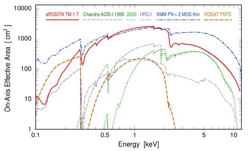
List of Tables
 3.1   Coordinates of the probed region . . . . . . . . . . . .      . . . . .   .   .    7
 3.2   Energy bands of eROSITA. . . . . . . . . . . . . . . .        . . . . .   .   .    8
 3.3   Wright et al. (2010) simplified WISE Criteria . . . . .       . . . . .   .   .   11
 3.4   Extinction values . . . . . . . . . . . . . . . . . . . . .   . . . . .   .   .   19
 3.5   Foreground star criteria based on isochrones . . . . . .      . . . . .   .   .   20
 3.6   Martin et al. (2004) selection of Canis Major sources in      2MASS       .   .   26
 3.7   Sources used for ECF calculation. . . . . . . . . . . . .     . . . . .   .   .   29

                                                                                         III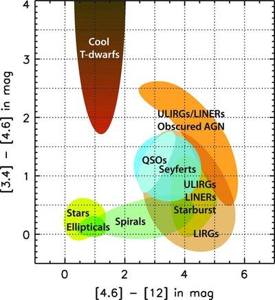
List of Figures
 2.1    Hertzsprung-Russell Diagram . . . . . .      . . . .   .   .   .   .   .   .   .   .   .   .   .    3
 2.2    Schematics of the eROSITA telescope . .      . . . .   .   .   .   .   .   .   .   .   .   .   .    4
 2.3    Effective areas of different X-ray surveys   . . . .   .   .   .   .   .   .   .   .   .   .   .    5
 2.4    X-ray image of the first eROSITA all-sky     survey.   .   .   .   .   .   .   .   .   .   .   .    6

 3.1    DSS image of the selected region of Canis Major . . . . . . . . . . .                               8
 3.2    Passbands of the Gaia, Skymapper, WISE and 2MASS surveys as
        function of wavelength . . . . . . . . . . . . . . . . . . . . . . . . .                           10
 3.3    WISE colour-colour diagram classification . . . . . . . . . . . . . .                              11
 3.4    WISE magnitude diagram . . . . . . . . . . . . . . . . . . . . . . .                               12
 3.5    Skymapper colour-magnitude diagram . . . . . . . . . . . . . . . .                                 12
 3.6    2MASS magnitude diagram . . . . . . . . . . . . . . . . . . . . . .                                13
 3.7    Skymapper g magnitude over X-ray count rate . . . . . . . . . . . .                                14
 3.8    Hardness Ratio diagram with Models . . . . . . . . . . . . . . . . .                               14
 3.9    X-ray count rate over HR1 . . . . . . . . . . . . . . . . . . . . . . .                            15
 3.10   X-ray count rate over HR2 . . . . . . . . . . . . . . . . . . . . . . .                            15
 3.11   Gaia and WISE counterpart comparison . . . . . . . . . . . . . . .                                 16
 3.12   Gaia colour magnitude diagram . . . . . . . . . . . . . . . . . . . .                              17
 3.13   Gaia G magnitude over estimated distance . . . . . . . . . . . . . .                               18
 3.14   Gaia G magnitude over eROSITA X-ray count rate . . . . . . . . .                                   18
 3.15   Comparison of two isochrones data bases . . . . . . . . . . . . . . .                              21
 3.16   Skymapper magnitude diagram with theoretical isochrones . . . . .                                  21
 3.17   2MASS magnitude diagram with highlighted foreground candidates
        based on the SM isochrone selection . . . . . . . . . . . . . . . . . .                            22
 3.18   Gaia magnitude diagram with highlighted foreground candidates
        based on the SM isochrone selection . . . . . . . . . . . . . . . . . .                            22
 3.19   Gaia magnitude diagram with theoretical isochrones . . . . . . . . .                               23
 3.20   2MASS magnitude diagram with highlighted foreground candidates
        based on the Gaia isochrone selection . . . . . . . . . . . . . . . . .                            23
 3.21   Skymapper magnitude diagram with highlighted foreground candi-
        dates based on the Gaia isochrone selection . . . . . . . . . . . . . .                            24
 3.22   2MASS magnitude diagram with theoretical isochrones . . . . . . .                                  24
 3.23   Gaia magnitude diagram with highlighted foreground candidates
        based on the 2MASS isochrone selection . . . . . . . . . . . . . . .                               25

                                                                                                           IV
List of Figures
3.24 Skymapper magnitude diagram with highlighted foreground candi-
dates based on the 2MASS isochrone selection . . . . . . . . . . . . 25
3.25 2MASS magnitude diagram with theoretical Canis Major isochrones
and the selection of Martin et al. (2004) . . . . . . . . . . . . . . . 27
3.26 RATE over HR1 diagram with only the matches meeting the Canis
Major criteria from Tab. 3.6. . . . . . . . . . . . . . . . . . . . . . 27
3.27 RATE over HR2 diagram with only the matches meeting the Canis
Major criteria in Tab. 3.6. . . . . . . . . . . . . . . . . . . . . . . . 28
3.28 Hardness Ratio diagram with models and only the matches meeting
the Canis Major criteria in Tab. 3.6 . . . . . . . . . . . . . . . . . . 28
3.29 X-ray-to-optical flux ratio over HR1 for all eROSITA-Skymapper
counterparts . . . . . . . . . . . . . . . . . . . . . . . . . . . . . . . 30
3.30 X-ray-to-optical flux ratio over HR2 for all eROSITA-Skymapper
counterparts . . . . . . . . . . . . . . . . . . . . . . . . . . . . . . . 30
3.31 X-ray-to-optical flux ratio over HR1 for all eROSITA-Gaia counter-
parts . . . . . . . . . . . . . . . . . . . . . . . . . . . . . . . . . . . 31
3.32 X-ray-to-optical flux ratio over HR2 for all eROSITA-Gaia counter-
parts . . . . . . . . . . . . . . . . . . . . . . . . . . . . . . . . . . . 31
3.33 Errors on the flux-ratio . . . . . . . . . . . . . . . . . . . . . . . . . 33
3.34 Errors on the hardness ratios . . . . . . . . . . . . . . . . . . . . . 33
3.35 X-ray-to-optical flux ratio for foreground candidates of eROSITA-
Skymapper data . . . . . . . . . . . . . . . . . . . . . . . . . . . . . 34
3.36 X-ray-to-optical flux ratio for background candidates of eROSITA-
Skymapper data . . . . . . . . . . . . . . . . . . . . . . . . . . . . . 35
3.37 X-ray-to-optical flux ratio for Normal Galaxy candidates of eROSITA-
Skymapper data . . . . . . . . . . . . . . . . . . . . . . . . . . . . . 35
3.38 X-ray-to-optical flux ratio for eROSITA-Skymapper data and Canis
Major candidates . . . . . . . . . . . . . . . . . . . . . . . . . . . . 37
3.39 X-ray-to-optical flux ratio for eROSITA-Skymapper data and likely
Canis Major sources . . . . . . . . . . . . . . . . . . . . . . . . . . 37
3.40 X-ray-to-optical flux ratio for eROSITA-Gaia data and likely Canis
Major sources . . . . . . . . . . . . . . . . . . . . . . . . . . . . . . 38
3.41 X-ray-to-optical flux ratio for eROSITA-Gaia data and likely Canis
Major sources . . . . . . . . . . . . . . . . . . . . . . . . . . . . . . 38
3.42 Hardness ratio diagram of Canis Major candidates . . . . . . . . . . 39
4.1 Missing Gaia counterparts . . . . . . . . . . . . . . . . . . . . . . . 45
4.2 Missing Skymapper counterparts . . . . . . . . . . . . . . . . . . . 46
4.3 Missing 2MASS counterparts . . . . . . . . . . . . . . . . . . . . . . 46
4.4 Missing WISE counterparts . . . . . . . . . . . . . . . . . . . . . . 47
V1 Introduction
Throughout the Universe, galaxies are never found as stand-alone objects but al-
ways in a minimum of pairs or clusters. They are not evenly distributed in space
but rather can be found in groups. Due to this characteristic, the evolution of
galaxies does not happen in isolation. Each galaxy interacts with several oth-
ers of their cohort through collisions or encounters during their lifetime. In the
case of smaller galaxies interacting with bigger ones, it is possible that tidal forces
rip the smaller one apart and merge it with the bigger one (Karttunen et al., 2017).
Regarding our Milky Way galaxy, 27 galaxies are associated with its subgroup
(McConnachie, 2012). Two well known satellite galaxies of the Milky Way are
the Large and Small Magellanic Clouds which are at a distance of about 60 kpc.
Computations suggest that those two satellites will merge with the Milky Way
during their next close approach (Karttunen et al., 2017). The closest known
satellite galaxy of the Milky Way is the Canis Major dwarf galaxy at a distance of
8 kpc (Martinez-Delgado et al., 2005).
The Canis Major dwarf Spheroidal Galaxy is an elliptical stellar overdensity in the
Canis Major constellation located at (l, b) = (240◦ , -8◦ ) and was first identified by
Martin et al. (2004). It is positioned close to the Galactic plane and believed to
be in the process of being pulled apart by gravitational forces of the Milky Way
galaxy. Its distance from the galactic centre is dGC = 12.0 kpc ± 1.2 kpc. There
was a M-giant overdensity detected which is similar in number to that in the core
of the Sagittarius dwarf galaxy. Because of that, it is assumed that the Canis
Major overdensity is an old dwarf satellite galaxy which is accreted onto the Milky
Way plane (Martin et al., 2004).
This work will pursue the findings of previous discoveries which are mostly based
on infrared observations to find more information about the population of the
Canis Major dwarf galaxy through X-ray observations.
12 Background Information
To gain a better understanding of the conducted research, this chapter conveys the
fundamental information about stellar evolution, X-ray sources and the eROSITA
mission.
2.1 Stellar Evolution
Stellar evolution begins in a gas cloud with the formation of a protostar. Depend-
ing on the accreted mass, either a planet, brown dwarf or main sequence star is
born. Lifespans of main sequence stars range from 107 to 1011 years depending on
their mass. Lower mass stars have a longer life span, more massive ones a shorter
one which also influences their path of life (Karttunen et al., 2017).
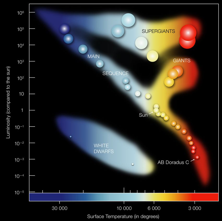
A Hertzsprung-Russell Diagram (HRD) as seen in Fig. 2.1 shows the luminosity
of stars as a function of effective temperature and thereby gives information about
their properties, masses, age and current stage in stellar evolution. The central
diagonal branch is called main sequence and consists of stars that fuse hydrogen
into helium. When their hydrogen supply is exhausted, they turn off the main se-
quence and turn into supergiants, giants or white dwarfs according to their initial
masses (ESO, 2007).
A low mass star starts on the main sequence with hydrogen core burning. This
phase is the longest and most stable stage in the life of a star and can be seen
in the HRD in Fig. 2.1 as a diagonal branch spanning across the diagram. After
all centre hydrogen is burned up, its main sequence phase comes to an end and
the star moves horizontally to the right in the HRD to the subgiant branch with
hydrogen shell burning. As the hydrogen shell burning increases its helium mass
and luminosity, the now so-called red giant moves upwards in the HRD. At the
end of this branch, there are several options. Stars which suffered from too much
mass loss will evolve directly into white dwarfs. If the stars’ mass is less than
than 2.3 M , the helium ignites and causes a flash in the core. This energy release
increases the temperature and expands the core of the star, moving it to the
horizontal branch. After the helium in the core is exhausted, the star reaches the
asymptotic giant branch, where burning of heavier elements can be realised. As
22 Background Information
Fig. 2.1: Hertzsprung-Russell Diagram showing the temperatures of stars against
their luminosities. Credit: ESO (2007)
soon as no more stages of burning can be ignited, its outer layers will be ejected
and become a planetary nebula with the remnant of the star being a white dwarf.
The white dwarf group can be found in the bottom left of the HRD.
Massive stars on the other end have a different fate. If their initial mass is bigger
than 8 M , the temperature in the core can reach higher temperatures thus being
able to do more extensive shell and core burning up to iron. When no more energy
is produced, there is also no gravity-counteracting pressure left and the core col-
lapses resulting in a supernova. Depending on the remaining mass, either a black
hole or a neutron star is formed (Karttunen et al., 2017).
32 Background Information
2.2 eROSITA Mission and X-Ray Sources
The extended ROentgen Survey with an Imaging Telescope Array (eROSITA) was
launched on the Russian Spektrum-Roentgen-Gamma (SRG) mission on July 13,
2019. The programme aims to perform eight all-sky surveys to provide the to date
most sensitive observations in soft X-rays (0.2–2.3 keV), and the first ever image
in hard X-rays (2.3–8 keV). This survey is called the eROSITA All-Sky Survey
(eRASS) and there will be eight surveys in total until 2023, each lasting half a
year (Predehl et al., 2021).
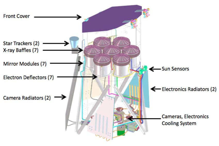
Fig. 2.2 shows the schematics of the eROSITA X-ray telescope. The core of the
telescope consists of seven identical mirror arrays with a charge-coupled-device
(CCD) camera in each focus point. Each CCD has 384x384 pixels with an image
area of 28.8 mm x 28.8 mm, the optimal operation temperature is at -85◦ C. In
order to protect the CCDs from cosmic particles, shields of copper and aluminium
are used. The mirrors are of the type Wolter-I, each a combination of 54 paraboloid
and hyperboloid mirrors which are especially used for X-ray telescopes. To coun-
teract the detection of photons from beyond the field of view, X-ray baffles are
placed in front of the mirror module (Predehl et al., 2021).
Fig. 2.2: Schematic of the eROSITA telescope. Labels show the name and quantity
of the parts. Taken from Merloni et al. (2012).
42 Background Information
The goal of the mission is to study the most massive structures and galaxy clusters
in the universe up to redshifts of z > 1 to test cosmological models including Dark
Energy, and to gain an improved set of X-ray data. The soft X-ray band (0.2–2.3
keV) will be 25 times more sensitive than the ROSAT All-Sky Survey and in the
X-ray hard band (2.3–8 keV), the first ever true imaging survey of the sky will
be completed with eROSITA. The extent of the energy band range compared to
other X-ray surveys can be found in Fig. 2.3 (Predehl et al., 2021).
Fig. 2.3: On–axis effective areas per energy band. eROSITA (red), Chandra ACIS-
I (green), Chandra HRC-I (purple), XMM-Newton (blue), and ROSAT
(brown) bands are plotted for comparison (Predehl et al., 2021).
New insights into other astrophysical phenomena linked with X-ray sources like
X-ray binaries, active stars, and diffuse emission within the Galaxy are expected
as well as the study of a few million active galactic nuclei (AGNs) to revolutionise
the view of supermassive black holes.
The first all-sky survey started on December 13, 2019. The resulting first image
of eROSITA can be found in Fig. 2.4 and shows some of the previously mentioned
X-ray phenomena very clearly. About one million X-ray sources have been de-
tected in this image. The whole sky is shown as Aitoff projection where the centre
of the Milky Way is in the middle. The detected photons have been colour-coded
according to their energy bands, with red representing 0.3 - 0.6 keV, green for 0.6 -
1 keV and blue for 1 - 2.3 keV. The red diffuse glow is emission of hot gas from the
Local Bubble, the blue emission in the galactic plane shows high-energy sources
52 Background Information
as low-energy emission is absorbed by dust and gas. Green and yellow colours
represent very hot gas which was rejected out of the galactic centre by supernovae
or the now dormant supermassive black hole in the centre of our galaxy among
other phenomena. This gas forms two huge bright bubbles in the halo above and
underneath the centre of the Milky Way. The southern part was firstly discovered
through eRASS1 and is together with the well-known northern bubble also known
as eROSITA bubbles. At the right edge of the blue galactic disc, the Vela super-
nova remnant can be seen in bright yellow. A lot of white X-ray point sources
like distant active galactic nuclei can be found uniformly distributed over the sky,
while galaxy clusters appear as extended X-ray nebulosities (MPE, 2020a,b).
Fig. 2.4: X-ray image of the first eROSITA all-sky survey. Photons have been
colour-coded according to their energy (red for 0.3 - 0.6 keV, green for
0.6 - 1 keV, blue for 1 - 2.3 keV). Credit: Jeremy Sanders, Hermann
Brunner and the eSASS team (MPE); Eugene Churazov, Marat Gilfanov
(on behalf of IKI)(MPE, 2020b).
63 Data Analysis
This chapter uses the data of the eROSITA all-sky survey 1 taken between 13
December 2019 and 11 June 2020 to analyse the region of the Canis Major dwarf
spheroidal galaxy.
3.1 eROSITA Catalogue
Two extraction regions as defined in Tab. 3.1 were selected according to Martin
et al. (2004) to cover the whole area of the Canis Major dwarf galaxy. The selected
region of the sky can be seen as yellow circles in a DSS survey image in Fig. 3.1.
RA[J2000] DEC[J2000] Radius (degree)
102.90207 -20.503367 13.2
111.2569 -34.829789 13.2
Tab. 3.1: Coordinates of the circular extraction regions of the Canis Major galaxy
based on Martin et al. (2004).
The eRASS1 catalogue was downloaded by Manami Sasaki from the eROSITA
data server. Afterwards, exclusively the sources which lie in the extraction region
of Tab. 3.1 were chosen via a script written by Manami Sasaki. There were 17 676
sources detected in the selected regions.
3.1.1 Catalogue Contents
The data from the eRASS1 catalogue includes the coordinates and observation IDs
of the sources. Furthermore, it provides even more information, including the total
number of X-ray counts per energy band i = 0, 1, 2, 3 as well as the corresponding
errors. The energy band widths of eROSITA can be found in Tab. 3.2. It also
contains the count rate for all energy bands which provides the number of counts
during a certain exposure time. In the following analysis, the total count rate of
i = 0 is referred to as RATE.
73 Data Analysis
Fig. 3.1: Selected regions of the Canis Major dwarf galaxy visualised by Sara Saeedi
in a DSS survey optical image. The two yellow circles mark the two chosen
extraction regions based on Tab. 3.1.
Band number i Energy Range [keV]
0 0.2-5.0
1 0.2-0.6
2 0.6-2.3
3 2.3-5.0
Tab. 3.2: Energy bands of eROSITA.
3.1.2 X-Ray Hardness Ratios
Hardness ratios (HR) are useful to compare the intensity of sources in different en-
ergy bands. They were calculated for the eROSITA X-ray data by using equations
3.1 and 3.2 in accordance with Saeedi et al. (2016). Instead of the count rates,
the number of counts Bi in each eROSITA band was used because this value is
more reliable as it shows the distribution of the total number of counts throughout
the energy bands. Bi is the softer band, Bi+1 the harder band, and EBi is the
83 Data Analysis
corresponding error of the counts. As there are three different energy bands in
eROSITA, two hardness ratios
Bi+1 − Bi
HRi = (3.1)
Bi+1 + Bi
and their corresponding errors
s
(Bi+1 · EBi )2 + (Bi · EBi+1 )2
EHRi = 2 · (3.2)
(Bi+1 + Bi )2
as seen in Saeedi et al. (2016) could be calculated which will be discussed later on
in section 3.2.1.
3.2 Multiwavelength Catalogues
The detected eROSITA X-ray sources were cross-matched with the optical Gaia
Data release 2 (Gaia Collaboration et al., 2016, 2018), the optical Skymapper
(SM) Data Release 1.1 (Wolf et al., 2018), The Wide-field Infrared Survey Ex-
plorer (WISE) catalogue (Cutri et al., 2014), and The Two Micron All Sky Sur-
vey (2MASS) near-infrared catalogue (Skrutskie et al., 2006) via a version of the
NWAY algorithm by Salvato et al. (2017) that was written by Jonathan Knies (Dr.
Karl Remeis-Observatory Bamberg).
The counterparts received by this provide important additional information about
the objects as an X-ray source may also have emission in other wavelengths. This
is the key feature of a population study as without this analysis, identification of
different types of objects would be difficult.
From the Gaia catalogue, Gaia’s white-light G-band (330–1050 nm), the blue (BP)
and red (RP) prismphotometers bands GBP ( 330–680 nm) and GRP (630–1050 nm)
were used as well as the estimated distance of sources. The Skymapper catalogue
provided data in its g (centre wavelength at 510 nm) and r (centre wavelength at
617 nm) bands, the WISE catalogue in W1 (3,4 µm), W2 (4,6 µm) and W3 (12 µm)
bands. 2MASS data was obtained in J (1,25 µm) and Ks (in the following called
K with 2,16 µm) bands. A visualization of the different passbands can be found
in Fig. 3.2. The analysis of the various diagrams made with this data will be
discussed in the following sections.
X-ray sources which didn’t have counterparts in certain catalogues were also plot-
ted for completeness and can be found in the Appendix.
93 Data Analysis
GBP G GRP
Gaia
normalized filter response [1]
g r
SkyMapper
W1 W2 W3
WISE
J K
2MASS
10000 105
Wavelength λ (Å)
Fig. 3.2: Passbands of the Gaia, Skymapper, WISE and 2MASS surveys as function
of wavelength. Created by Steven Hämmerich.
3.2.1 WISE Classification
The first step in identifying possible Canis Major sources was plotting the WISE
counterparts in a colour-magnitude diagram as seen in Fig. 3.4 and dividing them
in four different classes of sources based on Wright et al. (2010) (see Fig. 3.3
and Tab. 3.3). The four classification types are Galactic Foreground Sources and
Elliptical Galaxies (FE), Starburst Galaxies (SB), Active Galactic Nuclei (AGN),
and Normal Galaxies (NG). FE sources were marked in blue as they are very likely
to consist of stellar and therefore foreground sources. AGN and SB matches were
coloured in red for being potential background source. The remaining NG sources
were marked in black. Objects from the Canis Major dwarf galaxy can be expected
in the FE and NG classes as the galaxy is very close to the galactic plane and a
non-active elliptical normal galaxy.
This selection was highlighted in the magnitude diagrams of the counterparts of
the remaining catalogues.
103 Data Analysis
Fig. 3.3: WISE colour-colour diagram of different types of objects. W1 minus W2
band plotted over W2 minus W3 band where the bands are represented
in their respective wavelength (Wright et al., 2010).
Type W2-W3 [mag] W1-W2 [mag]
FE ≤ 1.5 ≤ 0.7
SB ≥ 4.6 ≤ 0.7
AGN > 0.7
NG 1.5 < W2-W3 < 4.6 ≤ 0.7
Tab. 3.3: Adjusted critical values of the WISE classification based on Fig. 3.3 by
Wright et al. (2010). The four classification types are Galactic Fore-
ground Sources and Elliptical Galaxies (FE), Starburst Galaxies (SB),
Active Galactic Nuclei (AGN), and Normal Galaxies (NG).
In the Skymapper magnitude diagram in Fig. 3.5, a separation between blue fore-
ground candidates and red background candidates becomes visible.
The 2MASS magnitude diagram in Fig. 3.6 also shows a separation between blue
foreground candidates and black normal galaxy candidates.
113 Data Analysis
Galactic Foreground Sources and Elliptical Galaxies
4 Background Candidates, Starburst
Background Candidates, AGNs
Normal Galaxies
3
2
W1-W2
1
0
1
4 2 0 2 4 6 8 10
W2-W3
Fig. 3.4: WISE magnitude diagram split in four different candidate types according
to the Wright et al. (2010) criteria in Tab. 3.3 and Fig. 3.3.
6 FE (WISE classification)
BC, SB (WISE classification)
BC, AGNs (WISE classification)
8 NG (WISE classification)
10
12
g
14
16
18
1.5 1.0 0.5 0.0 0.5 1.0 1.5 2.0
g-r
Fig. 3.5: Skymapper magnitude diagram with highlighted classes of objects accord-
ing to the Wright et al. (2010) criteria in Tab. 3.3 and Fig. 3.4.
123 Data Analysis
FE (WISE classification)
0.0 BC, SB (WISE classification)
BC, AGNs (WISE classification)
NG (WISE classification)
2.5
5.0
7.5
K
10.0
12.5
15.0
17.5
1 0 1 2 3 4
J-K
Fig. 3.6: 2MASS magnitude diagram with highlighted classes of objects according
to the Wright et al. (2010) criteria in Tab. 3.3 and Fig. 3.4.
Fig. 3.7 shows the comparison of the Skymapper g magnitude to the eROSITA
X-Ray countrate. The blue foreground candidates also appear to be separated
from the rest.
Furthermore, the hardness ratios calculated in section 3.1.2 are plotted in Fig. 3.8.
The sources are again coloured according to the WISE classification (see 3.3). The
diagram also shows various models of expected hardness ratio which were created
by Sara Saeedi via a PyXspec spectral analysis. Three power-law spectra (Γ =
1,2,3) and three black-body spectra (APEC at temperatures of kT = 0.2, 1.0 and
2.0 keV) models were chosen with different column densities (NH = 0.01·1022 cm−2
to 100·1022 cm−2 ) for correlation. The models only shown a small concordance
with the distribution of the sources. A cluster of sources lies in the bottom right
of Fig. 3.8 close to the dark green APEC model which suggests thermal emission
at low temperatures and low absorption. Moreover, the different types of sources
appear to be mixed and no clear separation is possible. This concludes that the
standard bands of eROSITA are not useful for further hardness ratio-based anal-
ysis.
Next, the calculated hardness ratios were compared to the total X-ray count rate
as seen in Fig. 3.9 and Fig. 3.10. Nearly all sources are soft X-ray sources as their
HR1 is mostly positive in Fig. 3.9 and HR2 mostly negative in Fig. 3.10.
133 Data Analysis
FE (WISE classification)
6 BC, SB (WISE classification)
BC, AGNs (WISE classification)
8 NG (WISE classification)
10
12
g (SM)
14
16
18
20
10 2 10 1 100
RATE
Fig. 3.7: Skymapper magnitudes in relation to the eROSITA X-Ray count rate.
The sources are highlighted according to the Wright et al. (2010) criteria
in Tab. 3.3 and Fig. 3.4.
100
1.00 kT = 0.2 keV
kT = 1.0 keV
kT = 2.0 keV
0.75 =1
=2
0.50 =3 0.5
FE (WISE classification)
0.01
0.25 BC, SB (WISE classification)
BCs, AGNs (WISE classification) 0.5
NG (WISE classification)
0.00
HR2
0.5
0.01
0.25 0.5
0.01
0.50
0.01
0.5
0.75 0.01
0.01
1.00 0.5
1.00 0.75 0.50 0.25 0.00 0.25 0.50 0.75 1.00
HR1
Fig. 3.8: HR diagram with power-law (Γ) and black-body (kT) spectra models.
Sources are highlighted according to the Wright et al. (2010) criteria in
Tab. 3.3 and Fig. 3.4. Column densities (NH ) are marked by crosses and
value in 1022 cm−2 . Median error on HR1 is 0.26 and 0.23 on HR2.
143 Data Analysis
103
FE (WISE classification)
BC, SB (WISE classification)
BC, AGNs (WISE classification)
102 NG (WISE classification)
101
RATE
100
10 1
10 2
1.0 0.5 0.0 0.5 1.0
HR1
Fig. 3.9: X-ray count rate over hardness ratio 1. The sources are highlighted ac-
cording to the Wright et al. (2010) criteria in Tab. 3.3 and Fig. 3.4.
103
FE (WISE classification)
BC, SB (WISE classification)
BC, AGNs (WISE classification)
102 NG (WISE classification)
101
RATE
100
10 1
10 2
1.0 0.5 0.0 0.5 1.0
HR2
Fig. 3.10: X-ray count rate over HR2. The sources are highlighted according to
the Wright et al. (2010) criteria in Tab. 3.3 and Fig. 3.4.
153 Data Analysis
3.2.2 Counterparts in the Gaia Catalogue
The retrieved optical Gaia counterparts were checked on reliability by calculating
the angular distance to the corresponding WISE counterpart. The 1-sigma posi-
tional error for each source can vary between 0.1” - 1.2” in the WISE catalogue.
If the position of the Gaia match differed from the position of the WISE match
by more than three times the 1-sigma positional error (≈ 3”), they were mostly
likely not the same source. This was done via small-angle approximations and the
equation for the distance between two points
p
γ = (DecW ISE − DecGaia )2 + (RAGaia − RAW ISE )2 (3.3)
and all matches with an angular distance γ < 3 ” were classified as reliable. The
rest was marked as unreliable as seen in Fig. 3.11. Furthermore, the different
classes of candidates were separated according to the magnitudes of their WISE
counterparts based on Wright et al. (2010).
Fig. 3.11 shows a linear correlation of the reliability of the matches which confirms
the assumption that some Gaia counterparts don’t match the original sources.
Those unreliable matches are marked in grey in every diagram that shows Gaia
data and were not considered in further classification.
5 >3
FE (WISE classification)
BC, SB (WISE classification)
0 BC, AGNs (WISE classification)
NG (WISE classification)
5
W1 (WISE)
10
15
20
0 5 10 15 20
G (Gaia)
Fig. 3.11: Gaia and WISE magnitude diagram for counterpart comparison. The
sources are highlighted according to the Wright et al. (2010) criteria in
Tab. 3.3 and Fig. 3.4. Unreliable sources based on Eq. 3.3 were marked
in grey.
163 Data Analysis
The different classes of candidates were further separated according to their mag-
nitude in the Gaia G band. Foreground candidates were narrowed down to those
counterparts which had G magnitude of less than 12. Background candidates were
narrowed down to those which had a G magnitude of more than 17. In general, it
is visible that the blue foreground candidates appear brighter than the red back-
ground candidates and are grouped in different regions of the diagram in Fig. 3.12,
Fig. 3.13, and also Fig. 3.14.
In the G-distance diagram in Fig. 3.13, also matches with an insufficient distance
significance are marked. They did not fulfil the equation for
p
u= χ2 /v (3.4)
according to Arenou et al. (2018) concerning the astrometric data where χ2 is
astrometric_chi2_al and v is astrometric_n_good_obs_al-5:
u < (1.2 · max(1, exp(−0.2 · (G − 19.5)))) (3.5)
They are also not used in the further analysis of Gaia data.
>3
2.5 FE, G>12
FE, G17
BC, SB, G17
7.5 BC, AGNs, G17
10.0 NG, G3 Data Analysis
>3
2.5 dist.sig criteria =false
FE, G>12
5.0 FE, G17
7.5 BC, SB, G17
BC, AGNs, G17
NG, G3
FE, G>12
5.0 FE, G17
BC, SB, G17
BC, AGNs, G17
NG, G3 Data Analysis
3.2.3 Isochrones
Isochrones show the evolutionary tracks of stars and indicate the position of a
stellar population in a colour-magnitude diagram depending on their age, metal-
licity and distance. Theoretical isochrones from the Dartmouth Stellar Evolution
Database based on Dotter et al. (2007, 2008) were plotted in the magnitude dia-
grams to compare the detected sources in the field of view of Canis Major with
theoretical values of galactic and Canis Major sources. As the stars of the Canis
major dwarf galaxy are observed to be quite old, a certain amount of sources are
expected to have turned off the main sequence and to be in the final stage of their
stellar evolution as explained in section 2.1.
For the theoretical isochrones of the Canis Major population, a metallicity of
Z = 0.00658, ages of τ = 2.5 Gyr, τ = 7 Gyr and τ = 15 Gyr and distances of
d = 5.5 kpc, d = 7 kpc and d = 8.5 kpc were chosen according to Martinez-Delgado
et al. (2005).
For galactic foreground candidates, the metallicity Z = 0.001925 of the Sun was
selected based on Vagnozzi (2019) to represent main sequence stars in our galactic
neighbourhood. In order to cover most possible foreground sources, distances of
d = 10 pc, d = 100 pc and d = 400 pc were plotted. To represent all populations
in these distances, the age of the galactic foreground population was chosen as
τ = 7.080 Gyr as the median age of the solar and disc age. Based on Grady et al.
(2020), ages of disc stars are at around τ = 10 Gyr, while the age of the Sun is
τ = 4.5 Gyr according to Bonanno et al. (2002).
The extinction A for galactic populations was set to 0 as the objects are part of the
Milky Way. The galactic extinction values of Canis Major in different wavelengths
are taken from the NASA/IPAC Extragalactic Database based on Schlafly and
Finkbeiner (2011) and can be found in Tab. 3.4. For Gaia magnitudes, no explicit
values were available, so the next closest available wavelength was chosen.
Survey g [mag] r [mag] J [mag] K [mag] BP [mag] RP [mag]
Skymapper 0.872 0.603
2MASS 0.187 0.080
Gaia 0.542 0.753 0.409
Tab. 3.4: Galactic extinction values A for Canis Major from NASA/IPAC Extra-
galactic Database based on Schlafly and Finkbeiner (2011).
193 Data Analysis
The expected apparent magnitudes m were calculated with the distance modulus
via the absolute magnitude M , distance d plus an additional extinction correction
factor A
m = M − [5 · (1 − log10 (d))] + A (3.6)
and plotted as isochrone curves in the Skymapper (Fig. 3.16), Gaia (Fig. 3.19)
and 2MASS (Fig. 3.22) colour-magnitude diagrams. The galactic isochrones fit
well within a distinguishable main sequence.
Likely galactic foreground populations were marked in all available magnitude di-
agrams along a cut that was set at the line where foreground candidates were not
any longer distinguishable from the other candidates and the theoretical Canis
Major isochrones. The line equations are given in Tab. 3.5.
Survey Cut
Skymapper g < (6.5 · (g − r) + 12)
g < (−10.4 · (g − r) + 23)
2MASS K < (6.1 · (J − K) + 10)
K < (−9.3 · (J − K) + 19.2)
Gaia G < (3.33 · (BP − RP ) + 11.67)
G < (−8.5 · (BP − RP ) + 27)
Tab. 3.5: Criteria to determine galactic foreground populations in magnitude di-
agrams. The line equations of the cuts between foreground candidates
and others are given in this table.
The Skymapper selection of likely foreground candidates was defined in Fig. 3.16
and highlighted in orange in the Gaia optical magnitude diagram in Fig. 3.18
and in the 2MASS magnitude diagram in Fig. 3.17. The coherency of different
data sets was also checked in Fig. 3.15. The data of the Padova database of
stellar evolutionary tracks and isochrones database1 and Dartmouth Stellar Evolu-
tion Database 2 match as expected. As the Dartmouth Stellar Evolution Database
provided data for all selected surveys, all isochrones were taken from there.
1
http://pleiadi.pd.astro.it/ (last visited on 11/04/2021)
2
http://stellar.dartmouth.edu/models/ (last visited on 11/04/2021)
203 Data Analysis
5
10
15
g
20
stellar.dartmouth.edu, Z=0.00658, age = 7Gyr, SM
stellar.dartmouth.edu, Z= 0.00816, age = 7Gyr, SDSS
25 pleiadi.oapd.inaf.it, Z=0.008 and age=7.08Gyr, SDSS
FE (WISE classification)
BC, SB (WISE classification)
BC, AGNs (WISE classification)
30 NG (WISE classification)
1.5 1.0 0.5 0.0 0.5 1.0 1.5 2.0
g-r
Fig. 3.15: Skymapper magnitudes with theoretical isochrones from two different
data bases which indeed overlap. The sources are highlighted according
to the Wright et al. (2010) criteria in Tab. 3.3 and Fig. 3.4.
2.5
Isochrone: Z=0.00658, 2.5 Gyr, 5.5 kpc
5.0 Isochrone: Z=0.00658, 2.5 Gyr, 7 kpc
Isochrone: Z=0.00658, 2.5 Gyr, 8.5 kpc
7.5 Isochrone: Z=0.00658, 7 Gyr, 5.5 kpc
Isochrone: Z=0.00658, 7 Gyr, 7 kpc
Isochrone: Z=0.00658, 7 Gyr, 8.5 kpc
10.0 Isochrone: Z=0.00658, 15 Gyr, 5.5 kpc
Isochrone: Z=0.00658, 15 Gyr, 7 kpc
Isochrone: Z=0.00658, 15 Gyr, 8.5 kpc
12.5
g
Galactic Iso.: Z=0.01925, 7 Gyr, 10 pc
Galactic Iso.: Z=0.01925, 7 Gyr, 100 pc
15.0 Galactic Iso.: Z=0.01925, 7 Gyr, 400 pc
FE (WISE classification)
BC, SB (WISE classification)
17.5 BC, AGNs (WISE classification)
NG (WISE classification)
20.0 Galactic Sources according to SM isochrones
0.50 0.25 0.00 0.25 0.50 0.75 1.00 1.25 1.50
g-r
Fig. 3.16: Skymapper magnitude diagram with theoretical isochrones. Galactic
sources based on Tab. 3.5. The sources are highlighted according to the
Wright et al. (2010) criteria in Tab. 3.3 and Fig. 3.4.
213 Data Analysis
0.0 Isochrone: Z=0.00658, 2.5 Gyr, 5.5 kpc
Isochrone: Z=0.00658, 2.5 Gyr, 7 kpc
2.5 Isochrone: Z=0.00658, 2.5 Gyr, 8.5 kpc
Isochrone: Z=0.00658, 7 Gyr, 5.5 kpc
5.0 Isochrone: Z=0.00658, 7 Gyr, 7 kpc
Isochrone: Z=0.00658, 7 Gyr, 8.5 kpc
Isochrone: Z=0.00658, 15 Gyr, 5.5 kpc
7.5 Isochrone: Z=0.00658, 15 Gyr, 7 kpc
Isochrone: Z=0.00658, 15 Gyr, 8.5 kpc
K
10.0 Galactic Iso.: Z=0.01925, 7 Gyr, 10 pc
Galactic Iso.: Z=0.01925, 7 Gyr, 100 pc
12.5 Galactic Iso.: Z=0.01925, 7 Gyr, 400 pc
FE (WISE classification)
BC, SB (WISE classification)
15.0 BC, AGNs (WISE classification)
NG (WISE classification)
17.5 Galactic Sources acc. to SM isochrones
20.0
0.5 0.0 0.5 1.0 1.5 2.0 2.5
J-K
Fig. 3.17: 2MASS magnitude diagram with highlighted foreground candidates
based on the Skymapper isochrone selection in Fig. 3.16. The sources
are highlighted according to the Wright et al. (2010) criteria in Tab. 3.3
and Fig. 3.4.
2.5
Isochrone: Z=0.00658, 2.5 Gyr, 5.5 kpc
5.0 Isochrone: Z=0.00658, 2.5 Gyr, 7 kpc
Isochrone: Z=0.00658, 2.5 Gyr, 8.5 kpc
Isochrone: Z=0.00658, 7 Gyr, 5.5 kpc
7.5 Isochrone: Z=0.00658, 7 Gyr, 7 kpc
Isochrone: Z=0.00658, 7 Gyr, 8.5 kpc
10.0 Isochrone: Z=0.00658, 15 Gyr, 5.5 kpc
Isochrone: Z=0.00658, 15 Gyr, 7 kpc
Isochrone: Z=0.00658, 15 Gyr, 8.5 kpc
12.5 Galactic Iso.: Z=0.01925, 7 Gyr, 10 pc
G
Galactic Iso.: Z=0.01925, 7 Gyr, 100 pc
15.0 Galactic Iso.: Z=0.01925, 7 Gyr, 400 pc
>3
17.5 FE (WISE classification)
BC, SB (WISE classification)
BC, AGNs (WISE classification)
20.0 NG (WISE classification)
Galactic Sources acc. to SM isochrones
22.5
1 0 1 2 3 4
BP-RP
Fig. 3.18: Gaia magnitude diagram with highlighted foreground candidates based
on the Skymapper isochrone selection in Fig. 3.16. The sources are
highlighted according to the Wright et al. (2010) criteria in Tab. 3.3
and Fig. 3.4.
223 Data Analysis
This procedure was repeated for the Gaia magnitudes. The likely galactic fore-
ground population was marked in olive in the Gaia optical magnitude diagram in
Fig. 3.19, and then highlighted in the magnitude diagrams of 2MASS in Fig. 3.20
and Skymapper in Fig. 3.21.
2.5
Isochrone: Z=0.00658, 2.5 Gyr, 5.5 kpc
5.0 Isochrone: Z=0.00658, 2.5 Gyr, 7 kpc
Isochrone: Z=0.00658, 2.5 Gyr, 8.5 kpc
Isochrone: Z=0.00658, 7 Gyr, 5.5 kpc
7.5 Isochrone: Z=0.00658, 7 Gyr, 7 kpc
Isochrone: Z=0.00658, 7 Gyr, 8.5 kpc
10.0 Isochrone: Z=0.00658, 15 Gyr, 5.5 kpc
Isochrone: Z=0.00658, 15 Gyr, 7 kpc
Isochrone: Z=0.00658, 15 Gyr, 8.5 kpc
12.5 Galactic Iso.: Z=0.01925, 7 Gyr, 10 pc
G
Galactic Iso.: Z=0.01925, 7 Gyr, 100 pc
15.0 Galactic Iso.: Z=0.01925, 7 Gyr, 400 pc
>3
17.5 FE (WISE classification)
BC, SB (WISE classification)
BC, AGNs (WISE classification)
20.0 NG (WISE classification)
Galactic Sources acc. to Gaia isochrones
22.5
1 0 1 2 3 4
BP-RP
Fig. 3.19: Gaia magnitude diagram with theoretical isochrones. Galactic sources
based on Tab. 3.5. The sources are highlighted according to the Wright
et al. (2010) criteria in Tab. 3.3 and Fig. 3.4.
0.0 Isochrone: Z=0.00658, 2.5 Gyr, 5.5 kpc
Isochrone: Z=0.00658, 2.5 Gyr, 7 kpc
2.5 Isochrone: Z=0.00658, 2.5 Gyr, 8.5 kpc
Isochrone: Z=0.00658, 7 Gyr, 5.5 kpc
5.0 Isochrone: Z=0.00658, 7 Gyr, 7 kpc
Isochrone: Z=0.00658, 7 Gyr, 8.5 kpc
Isochrone: Z=0.00658, 15 Gyr, 5.5 kpc
7.5 Isochrone: Z=0.00658, 15 Gyr, 7 kpc
Isochrone: Z=0.00658, 15 Gyr, 8.5 kpc
K
10.0 Galactic Iso.: Z=0.01925, 7 Gyr, 10 pc
Galactic Iso.: Z=0.01925, 7 Gyr, 100 pc
12.5 Galactic Iso.: Z=0.01925, 7 Gyr, 400 pc
FE (WISE classification)
BC, SB (WISE classification)
15.0 BC, AGNs (WISE classification)
NG (WISE classification)
17.5 Galactic Sources acc. to Gaia isochrones
20.0
0.5 0.0 0.5 1.0 1.5 2.0 2.5
J-K
Fig. 3.20: 2MASS magnitude diagram with highlighted foreground candidates
based on the Gaia isochrone selection in Fig. 3.19. The sources are
highlighted according to the criteria in Tab. 3.3 and Fig. 3.4.
233 Data Analysis
2.5
Isochrone: Z=0.00658, 2.5 Gyr, 5.5 kpc
5.0 Isochrone: Z=0.00658, 2.5 Gyr, 7 kpc
Isochrone: Z=0.00658, 2.5 Gyr, 8.5 kpc
7.5 Isochrone: Z=0.00658, 7 Gyr, 5.5 kpc
Isochrone: Z=0.00658, 7 Gyr, 7 kpc
Isochrone: Z=0.00658, 7 Gyr, 8.5 kpc
10.0 Isochrone: Z=0.00658, 15 Gyr, 5.5 kpc
Isochrone: Z=0.00658, 15 Gyr, 7 kpc
Isochrone: Z=0.00658, 15 Gyr, 8.5 kpc
12.5
g
Galactic Iso.: Z=0.01925, 7 Gyr, 10 pc
Galactic Iso.: Z=0.01925, 7 Gyr, 100 pc
15.0 Galactic Iso.: Z=0.01925, 7 Gyr, 400 pc
FE (WISE classification)
BC, SB (WISE classification)
17.5 BC, AGNs (WISE classification)
NG (WISE classification)
20.0 Galactic Sources acc. to Gaia isochrones
0.50 0.25 0.00 0.25 0.50 0.75 1.00 1.25 1.50
g-r
Fig. 3.21: Skymapper magnitude diagram with highlighted foreground candidates
based on the Gaia isochrone selection in Fig. 3.19. The sources are
highlighted according to the Wright et al. (2010) criteria in Tab. 3.3
and Fig. 3.4.
Lastly, the likely foreground population in the 2MASS magnitude diagram was
identified in Fig. 3.22. This selection was then highlighted in green in the magni-
tude diagrams of Gaia in Fig. 3.23 and Skymapper in Fig. 3.24.
0.0 Isochrone: Z=0.00658, 2.5 Gyr, 5.5 kpc
Isochrone: Z=0.00658, 2.5 Gyr, 7 kpc
2.5 Isochrone: Z=0.00658, 2.5 Gyr, 8.5 kpc
Isochrone: Z=0.00658, 7 Gyr, 5.5 kpc
5.0 Isochrone: Z=0.00658, 7 Gyr, 7 kpc
Isochrone: Z=0.00658, 7 Gyr, 8.5 kpc
Isochrone: Z=0.00658, 15 Gyr, 5.5 kpc
7.5 Isochrone: Z=0.00658, 15 Gyr, 7 kpc
Isochrone: Z=0.00658, 15 Gyr, 8.5 kpc
K
10.0 Galactic Iso.: Z=0.01925, 7 Gyr, 10 pc
Galactic Iso.: Z=0.01925, 7 Gyr, 100 pc
12.5 Galactic Iso.: Z=0.01925, 7 Gyr, 400 pc
FE (WISE classification)
BC, SB (WISE classification)
15.0 BC, AGNs (WISE classification)
NG (WISE classification)
17.5 Galactic Sources acc. to 2mass isochrones
20.0
0.5 0.0 0.5 1.0 1.5 2.0 2.5
J-K
Fig. 3.22: 2MASS magnitude diagram with theoretical isochrones. Galactic sources
based on Tab. 3.5. The sources are highlighted according to the Wright
et al. (2010) criteria in Tab. 3.3 and Fig. 3.4.
243 Data Analysis
2.5
Isochrone: Z=0.00658, 2.5 Gyr, 5.5 kpc
5.0 Isochrone: Z=0.00658, 2.5 Gyr, 7 kpc
Isochrone: Z=0.00658, 2.5 Gyr, 8.5 kpc
Isochrone: Z=0.00658, 7 Gyr, 5.5 kpc
7.5 Isochrone: Z=0.00658, 7 Gyr, 7 kpc
Isochrone: Z=0.00658, 7 Gyr, 8.5 kpc
10.0 Isochrone: Z=0.00658, 15 Gyr, 5.5 kpc
Isochrone: Z=0.00658, 15 Gyr, 7 kpc
Isochrone: Z=0.00658, 15 Gyr, 8.5 kpc
12.5 Galactic Iso.: Z=0.01925, 7 Gyr, 10 pc
G
Galactic Iso.: Z=0.01925, 7 Gyr, 100 pc
15.0 Galactic Iso.: Z=0.01925, 7 Gyr, 400 pc
>3
17.5 FE (WISE classification)
BC, SB (WISE classification)
BC, AGNs (WISE classification)
20.0 NG (WISE classification)
Galactic Sources acc. to 2mass isochrones
22.5
1 0 1 2 3 4
BP-RP
Fig. 3.23: Gaia magnitude diagram with highlighted foreground candidates based
on the 2MASS isochrone selection in Fig. 3.22. The sources are high-
lighted according to the Wright et al. (2010) criteria in Tab. 3.3 and
Fig. 3.4.
2.5
Isochrone: Z=0.00658, 2.5 Gyr, 5.5 kpc
5.0 Isochrone: Z=0.00658, 2.5 Gyr, 7 kpc
Isochrone: Z=0.00658, 2.5 Gyr, 8.5 kpc
7.5 Isochrone: Z=0.00658, 7 Gyr, 5.5 kpc
Isochrone: Z=0.00658, 7 Gyr, 7 kpc
Isochrone: Z=0.00658, 7 Gyr, 8.5 kpc
10.0 Isochrone: Z=0.00658, 15 Gyr, 5.5 kpc
Isochrone: Z=0.00658, 15 Gyr, 7 kpc
Isochrone: Z=0.00658, 15 Gyr, 8.5 kpc
12.5
g
Galactic Iso.: Z=0.01925, 7 Gyr, 10 pc
Galactic Iso.: Z=0.01925, 7 Gyr, 100 pc
15.0 Galactic Iso.: Z=0.01925, 7 Gyr, 400 pc
FE (WISE classification)
BC, SB (WISE classification)
17.5 BC, AGNs (WISE classification)
NG (WISE classification)
20.0 Galactic Sources acc. to 2mass isochrones
0.50 0.25 0.00 0.25 0.50 0.75 1.00 1.25 1.50
g-r
Fig. 3.24: Skymapper magnitude diagram with highlighted foreground candidates
based on the 2MASS isochrone selection in Fig. 3.22. The sources are
highlighted according to the Wright et al. (2010) criteria in Tab. 3.3 and
Fig. 3.4.
253 Data Analysis
The comparison of foreground candidate selections of the different surveys con-
cludes that the selections are mostly focused on the same region in every magnitude
diagram. All selected galactic candidates lie in the upper part of the main sequence
which supports the theory of them being foreground stars. This is observable in
all magnitude diagrams and therefore these counterparts are very likely to be fore-
ground objects. But, there is one noticeable aberration in the 2MASS colour-colour
diagrams. The selection of foreground candidates based on the 2MASS isochrones
in Fig. 3.22 is not completely in accordance with the selection based on Skymap-
per and Gaia isochrones in Fig. 3.17 and 3.20 as the selections based on Gaia and
Skymapper both do not include sources above J-K bigger than approximately 0.8
mag. Henceforth, the Skymapper isochrone criteria in Tab. 3.5 will be used to
identify foreground candidates in 2MASS diagrams as this selection appears more
precise than the one based on the 2MASS isochrones.
3.2.4 2MASS Criteria
Martin et al. (2004) identified two areas of Canis Major population in 2MASS
data as seen in Tab. 3.6, the Giant Branch which is explained in section 2.1, and
the Red Clump. Red Clump stars are low-mass stars in their core-helium-burning
stage and form a notably prominent cluster next to the red giant branch. The
sources identified as part of the Giant Branch and Red Clump by this criteria were
marked in the 2MASS magnitude diagram in Fig. 3.25 and plotted in diagrams of
eROSITA data. The X-ray count rate over the two hardness ratios can be found
in Fig. 3.26 and Fig. 3.27. The hardness ratio diagram is in Fig. 3.28. These
diagrams don’t provide a lot of new insights. The sources appear to be mostly
soft X-ray sources based on their mostly positive HR1, and mainly negative HR2.
The hardness ratio diagram in Fig. 3.28 still shows only a slight correlation with
the hardness ratio models and suggests that most sources are thermal emitting as
indicated by the green APEC model with a low temperature (kT around 0.2 to 1
keV) and low absorption as discussed earlier in section 3.2.1.
Class J-K [mag] Criteria K [mag] Criteria
Giant Branch 0.807 < J-K < 1.307 8.08 < K < 12.08
Red Clump 0.657 < J-K < 0.757 12.08 < K < 13.58
Tab. 3.6: Martin et al. (2004) selection of Canis Major sources respecting the galac-
tic extinction from Tab. 3.4 which was corrected in the paper but not in
the data used here.
263 Data Analysis
4
Isochrone: Z=0.00658, 2.5 Gyr, 5.5 kpc
Isochrone: Z=0.00658, 2.5 Gyr, 7 kpc
Isochrone: Z=0.00658, 2.5 Gyr, 8.5 kpc
6 Isochrone: Z=0.00658, 7 Gyr, 5.5 kpc
Isochrone: Z=0.00658, 7 Gyr, 7 kpc
Isochrone: Z=0.00658, 7 Gyr, 8.5 kpc
Isochrone: Z=0.00658, 15 Gyr, 5.5 kpc
8 Isochrone: Z=0.00658, 15 Gyr, 7 kpc
Isochrone: Z=0.00658, 15 Gyr, 8.5 kpc
Galactic Iso.: Z=0.01925, 7 Gyr, 10 pc
K
10 Galactic Iso.: Z=0.01925, 7 Gyr, 100 pc
Galactic Iso.: Z=0.01925, 7 Gyr, 400 pc
FE (WISE classification)
BC, SB (WISE classification))
12 BC, AGNs (WISE classification)
NG (WISE classification)
Galactic Sources according to SM isochrones
Giant Branch (Martin et al., 2004)
14 Red Clump (Martin et al., 2004)
0.2 0.0 0.2 0.4 0.6 0.8 1.0 1.2 1.4
J-K
Fig. 3.25: 2MASS magnitude diagram with theoretical Canis Major isochrones and
the selection of Martin et al. (2004) (Tab. 3.25) marked in pink. The
rest of the sources are marked based on Tab. 3.3 and Fig. 3.4.
103
Giant Branch (Martin et al., 2004)
Red Clump (Martin et al., 2004)
102
101
RATE
100
10 1
10 2
1.0 0.5 0.0 0.5 1.0
HR1
Fig. 3.26: RATE over HR1 diagram with only the matches meeting the Canis Ma-
jor criteria from Tab. 3.6.
273 Data Analysis
103
Giant Branch (Martin et al., 2004)
Red Clump (Martin et al., 2004)
102
101
RATE
100
10 1
10 2
1.0 0.5 0.0 0.5 1.0
HR2
Fig. 3.27: RATE over HR2 diagram with only the matches meeting the Canis Ma-
jor criteria in Tab. 3.6.
100
1.00 kT = 0.2 keV
kT = 1.0 keV
kT = 2.0 keV
0.75 =1
=2
0.50 =3 0.5
Giant Branch (Martin et al. 2004)
0.01
0.25 Red Clump (Martin et al., 2004)
0.5
0.00
HR2
0.5
0.01
0.25 0.5
0.01
0.50
0.01
0.5
0.75 0.01
0.01
1.00 0.5
1.00 0.75 0.50 0.25 0.00 0.25 0.50 0.75 1.00
HR1
Fig. 3.28: HR diagram with hardness ratio models and only the matches meeting
the Canis Major criteria in Tab. 3.6. Models are the same as Fig. 3.8.
Column densities (NH ) are marked by crosses and value in 1022 cm−2 .
Median errors on HR1 and HR2 are 0.26 and 0.23 respectively.
283 Data Analysis
3.2.5 Analysis of X-Ray Properties
From the selection in section 3.2.4, five of the nine brightest sources were picked for
further analysis. Sara Saeedi provided a spectral analysis of eROSITA data where
the spectrum for each source was extracted and fitted with a spectral model. This
method made it possible to find the conversion factor between the count rate
measured with eROSITA and the real flux of the source. The energy conversion
factor (ECF) was computed by using Eq. 3.7 from Saeedi et al. (2016). With the
ECF, it was possible to calculate the estimated flux
RAT E
Fx = (3.7)
ECF
for all sources. The ECF values of the sources in Tab. 3.7 were averaged and
yielded a value of ECF = 3.46e11. The spectral analysis by Sara Saeedi suggests
that sources 4, 5 and 7 are foreground stars, 6 and 8 are unclear.
Number Net count rate (cts/s) Flux (0.2–5.0 keV)
4 1.636 4.6931e-12
5 2.4931 6.9505e-12
7 1.348 4.1138e-12
Tab. 3.7: Sources used for ECF calculation.
Next, the X-ray-to-optical flux ratio
Fx m1 + m2
log = log10 (Fx ) + + 5.37 (3.8)
Fopt 2 · 2.5
was calculated according to Saeedi et al. (2016) to separate optically bright sources
from bright X-ray sources. The equation was slightly modified by replacing the
SDSS9 bands with m1 and m2 , where m1 refers to the g band in Skymapper and
BP in Gaia, and m2 refers to the Skmapper r band and Gaia RP band respectively.
The X-ray-to-optical flux ratio as function of the hardness ratios can be found in
Fig. 3.29 and Fig. 3.30 for Skymapper magnitudes, and Fig. 3.31 and Fig. 3.32
for Gaia magnitudes.
293 Data Analysis
FE (WISE classification)
BC, SB (WISE classification)
1 BC, AGNs (WISE classification)
NG (WISE classification)
Galactic Sources according to SM isochrones
0
log(Fx/Fopt(SM))
1
2
3
4
5
1.00 0.75 0.50 0.25 0.00 0.25 0.50 0.75 1.00
HR1
Fig. 3.29: X-ray-to-optical flux ratio for all eROSITA-SM counterparts. The
sources are highlighted according to the Wright et al. (2010) criteria
in Tab. 3.3 and Fig. 3.4 and to the isochrone criteria in Fig. 3.16.
FE (WISE classification)
BC, SB (WISE classification)
1 BC, AGNs (WISE classification)
NG (WISE classification)
Galactic Sources according to SM isochrones
0
log(Fx/Fopt(SM))
1
2
3
4
5
1.00 0.75 0.50 0.25 0.00 0.25 0.50 0.75 1.00
HR2
Fig. 3.30: X-ray-to-optical flux ratio for all eROSITA-SM counterparts. The
sources are highlighted according to the Wright et al. (2010) criteria
in Tab. 3.3 and Fig. 3.4 and to the isochrone criteria in Fig. 3.16.
303 Data Analysis
2
0
log(Fx/Fopt(Gaia))
>3
2 FE, G>12
FE, G17
BC, SB, G17
BC, AGNs, G17
NG, G3
2 FE, G>12
FE, G17
BC, SB, G17
BC, AGNs, G17
NG, G3 Data Analysis
In order to get the error on the flux ratio, the error on the RATE, which is defined
as
B0
RAT E = (3.9)
exposure
had to be calculated :
s 2 s 2
1 RAT E
4RAT E = · EB02 = · EB02 . (3.10)
exposure B0
with the total counts B0 , and their corresponding errors EB0 for the error of the
RATE. Including the error of the magnitudes 4mi , the error on the X-ray-to-
optical flux ratio added up to:
s 2
Fx 1 1 1
4 log = · 4RAT E 2 + 4m21 + · 4m22 (3.11)
Fopt ln(10) · RAT E 25 25
The error bars of the X-ray-to-optical flux ratio can be found in Fig. 3.33. To
get a hint of the dimension of the hardness ratio errors, Fig. 3.34 shows the hard-
ness ratio diagram of likely Canis Major sources with corresponding error bars as
calculated in Eq. 3.2. The errors of the hardness ratio vary a lot and should be
closer considered in further work with specific sources. The median error on HR1
is 0.26, the median error on HR2 is 0.23.
323 Data Analysis
Giant Branch (Martin et al., 2004)
Red Clump (Martin et al., 2004)
1
0
log(Fx/Fopt(SM))
1
2
3
4
5
1.00 0.75 0.50 0.25 0.00 0.25 0.50 0.75 1.00
HR1
Fig. 3.33: X-ray-to-optical flux ratio for eROSITA-Skymapper data and likely Ca-
nis Major sources according to Tab. 3.25 with error bars for the flux-
ratio.
2.0 Giant Branch (Martin et al., 2004)
Red Clump (Martin et al., 2004)
1.5
1.0
0.5
0.0
HR2
0.5
1.0
1.5
2.0
2.0 1.5 1.0 0.5 0.0 0.5 1.0 1.5 2.0
HR1
Fig. 3.34: Hardness Ratio diagram of likely Canis Major sources according to Tab.
3.25 with error bars. The median values of the errors on HR1 and HR2
are 0.26 and 0.23 respectively.
333 Data Analysis
Fig. 3.33 shows that the Canis Major sources appear to be distributed around
log FFopt
x
= -1 in comparison to Skymapper optical magnitudes. Background
sources like X-ray binaries are at log FFopt
x
= 0 in Fig. 3.36 and Fig. 3.37 be-
cause they are bright in X-ray.
On the other hand, galactic foreground sources like stars can be found below
log FFopt
x
= -2 in Fig. 3.35. They are less bright in X-ray but especially bright in
optical magnitudes which supports the foreground star theory for those counter-
parts.
FE (WISE classification)
Galactic Sources according to SM isochrones
1
0
log(Fx/Fopt(SM))
1
2
3
4
5
1.00 0.75 0.50 0.25 0.00 0.25 0.50 0.75 1.00
HR1
Fig. 3.35: X-ray-to-optical flux ratio for foreground candidates of eROSITA-SM
data. The sources are highlighted according to the WISE criteria in
Tab. 3.3 and Fig. 3.4 and to the isochrone criteria in Fig. 3.16.
343 Data Analysis
BC, Starburst (WISE classification)
BC, AGNs (WISE classification)
1 Galactic Sources according to SM isochrones
0
log(Fx/Fopt(SM))
1
2
3
4
5
1.00 0.75 0.50 0.25 0.00 0.25 0.50 0.75 1.00
HR1
Fig. 3.36: X-ray-to-optical flux ratio for background candidates of eROSITA-SM
data. The sources are highlighted according to the WISE criteria in Tab.
3.3 and Fig. 3.4 and to the isochrone criteria in Fig. 3.16.
NG (WISE classification)
Galactic Sources according to SM isochrones
1
0
log(Fx/Fopt(SM))
1
2
3
4
5
1.00 0.75 0.50 0.25 0.00 0.25 0.50 0.75 1.00
HR1
Fig. 3.37: X-ray-to-optical flux ratio for Normal Galaxy candidates of eROSITA-
SM data. The sources are highlighted according to the WISE criteria in
Tab. 3.3 and Fig. 3.4 and to the isochrone criteria in Fig. 3.16.
353 Data Analysis
3.3 Final Classification
The final step in the population study of the Canis Major dwarf spheroidal galaxy
is combining the results from the previous analysis. In order to do this, the se-
lected sources from Martin et al. (2004) in section 3.2.4 were singled out and further
analysed by the WISE, Gaia and isochrone criteria. Canis Major candidates were
marked in the following diagrams by dots, foreground candidates by crosses.
The selected sources were plotted in X-ray-to-optical flux ratio diagrams as intro-
duced in section 3.2.5. Foreground candidates were located below log FFopt
x
= -2,
Fx
while Canis Major candidates were situated around log Fopt = -1. This pattern
can also be observed in the selection of Martin et al. in Fig. 3.38 to Fig. 3.41
where clear foreground star candidates can be found in the lower part of the dia-
gram due to their brightness in optical magnitudes.
From the first and most helpful WISE classification in section 3.2.1, a lot of con-
clusions could be drawn. The WISE classification identified background (BC),
foreground stars and elliptical galaxies (FE) and normal galaxy (NG) candidates
and were marked accordingly in the final selection. Most counterparts in Fig. 3.38
to Fig. 3.41 belong to the foreground stars and elliptical galaxies class which is in
accordance with the position and type of the Canis Major galaxy.
The isochrone criteria from section 3.2.3 was used to highlight high probability
foreground candidates. Orange crosses in Fig. 3.38 and in Fig. 3.39 mark fore-
ground candidates that were derived from the position of the theoretical isochrones
in the Skymapper colour-magnitude diagram in Fig. 3.16. Green crosses in Fig.
3.40 and in Fig. 3.41 were taken from the optical Gaia isochrones in Fig. 3.19.
These sources lie above the intersection with the Canis Major isochrones on the
main sequence of the optical colour-magnitude diagrams. Thus, they qualify as
highly likely foreground candidates and won’t be taken in the final selection of
Canis Major candidates.
Another criteria which can be considered through counterparts from the Gaia cat-
alogue is the value of magnitude. In section 3.2.2, it was discussed that Gaia
matches with a G-magnitude of less than 12 are very likely foreground candidates.
These counterparts were marked as light blue crosses in Fig. 3.40 and 3.41, and
also not considered as Canis Major sources.
363 Data Analysis
Fg Candidates acc. to SM isochrones
FE (WISE classification)
1 BC (WISE classification)
NG (WISE classification)
0
log(Fx/Fopt(SM))
1
2
3
4
5
1.00 0.75 0.50 0.25 0.00 0.25 0.50 0.75 1.00
HR1
Fig. 3.38: X-ray-to-optical flux ratio for eROSITA-SM data and likely Canis Major
sources. The sources are highlighted according to the WISE criteria in
Tab. 3.3 and Fig. 3.4 and to the isochrone criteria in Fig. 3.16.
Fg Candidates acc. to SM isochrones
FE (WISE classification)
1 BC (WISE classification)
NG (WISE classification)
0
log(Fx/Fopt(SM))
1
2
3
4
5
1.00 0.75 0.50 0.25 0.00 0.25 0.50 0.75 1.00
HR2
Fig. 3.39: X-ray-to-optical flux ratio for eROSITA-SM data and likely Canis Major
sources. The sources are highlighted according to the WISE criteria in
Tab. 3.3 and Fig. 3.4 and to the isochrone criteria in Fig. 3.16.
37You can also read