A Graphical EDA Tool with ggplot2: brinton - The R Journal
←
→
Page content transcription
If your browser does not render page correctly, please read the page content below
C ONTRIBUTED RESEARCH ARTICLE                                                                                             321

          A Graphical EDA Tool with ggplot2:
          brinton
          by Pere Millán-Martínez, Ramon Oller

          Abstract We present brinton package, which we developed for graphical exploratory data analysis in
          R. Based on ggplot2, gridExtra and rmarkdown, brinton package introduces wideplot() graphics for
          exploring the structure of a dataset through a grid of variables and graphic types. It also introduces
          longplot() graphics, which present the entire catalog of available graphics for representing a particular
          variable using a grid of graphic types and variations on these types. Finally, it introduces the plotup()
          function, which complements the previous two functions in that it presents a particular graphic for a
          specific variable of a dataset. This set of functions is useful for understanding the structure of a data
          set, discovering unexpected properties in the data, evaluating different graphic representations of
          these properties, and selecting a particular graphic for display on the screen.

          Introduction

          In 1977, J.W. Tukey noted that “The greatest value of a picture is when it forces us to notice what we
          never expected to see” (Tukey, 1977, p.iv). This statement aligns with expectation disconfirmation
          theory (Oliver, 1977), which links consumers’ satisfaction to their expectations. The field of exploratory
          data analysis (EDA) is characterized precisely by not requiring an expectation, since in this approach
          hypotheses may not be pre-established. Rather, they are allowed to emerge through the observation
          of the data. Additionally, because we cannot automate the processes of defining a problem or the
          corresponding hypotheses —as signaled by J. Bertin that same year (Bertin, 1977, p.2)—, we face
          the challenge of automating graphical representations so that users can examine the data, develop
          hypotheses and then select the appropriate statistical graphic that will enable them to satisfy their
          recently created expectations.
              The tools for generating graphics and statistics for a dataset automatically are called automated
          exploratory data analysis or autoEDA (Staniak and Biecek, 2019). These tools facilitate some of
          the characteristic tasks of EDA, such as describing variables and validating observations or the
          relationships established between the values of one or more variables. brinton, a new package we
          have developed for use within R, shows only graphics, leading us to classify it as a tool for automated
          graphical exploratory data analysis or autoGEDA. We can include in this category tools such as GGobi
          (Cook et al., 2007) and Mondrian (Theus and Urbanek, 2008). These tools differ from brinton in that
          they use interactive techniques extensively, and therefore are usually classified as visual analytics.
               Multiple strategies exist for automating statistical diagramatic representations. Millán-Martínez
          and Valero-Mora (2018) differentiate strategies according to whether they are based on the character-
          istics of the data (functional design, Kamps (1999)), on the habits of a group of users (collaborative
          filtering), on those of a single user (content-based filtering), on the tasks that the user is meant to
          perform (task design), on the characteristics of human perception (perceptual design), on the limita-
          tions of the communication channel or the screen on which the graphics are projected (responsive
          design), or, finally, on the selection of characteristics of the desired graphics or models of representation
          (representation model design or deterministic design).
              The statistical programming environment R has two graphics systems (Friendly, 2018). One is
          the standard graphics system of the package graphics with low-level functions, such as lines(),
          points(), legend() (which define concrete elements of a graphic) and high-level functions, such
          as plot(), pie(), and barplot() (which present a complete graphic). The other graphics system is
          based on the grid package, with low-level functions such as those of the gridExtra package (Auguie,
          2017) and high-level ones such as those of the packages lattice (Sarkar, 2008) and ggplot2 (Wickham,
          2016), which produce complete graphics. Both in graphics and grid we find examples of the strategies
          mentioned above. We find functional design, for example, in the plot() function. If we apply it to
          the dataset cars, it produces a scatterplot, because it contains two numerical variables and is of the
          data.frame class. If we apply it to the dataset airmiles, it produces a line graph because this dataset
          has a single numerical variable and is of the ts class. We find task design in multiple packages, for
          example survminer (Therneau, 2015), which includes the function ggsurvplot() to generate graphics
          specifically for survival analysis. We find representation model design in basic functions such as
          barplot(), which produces a bar graph; hist(), which produces a histogram; and pie(), which
          produces a pie chart. We also see lower-level functions, such as the geom_point() function of ggplot2,
          which reduces the graphic to a kind of point plot. We can also find in ggplot2 examples of perceptual
          design in decisions such as the default size, shape and color of the points, the grid lines and the panel

          The R Journal Vol. 12/2, December 2020                                                    ISSN 2073-4859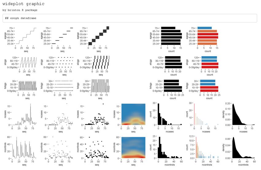
C ONTRIBUTED RESEARCH ARTICLE                                                                                        322

          background.
              Despite all of the solutions already implemented in R, we are lacking an approach based on
          functional design that uses higher-level functions to show systematically not only a complete graphic
          but also a wide range of available graphics using the same data. Examining multiple graphics could
          lead the user to raise questions, which he or she could then answer using the presented graphics,
          new more specific graphics, or a particular graphic that could be adapted as needed (deterministic
          design). brinton package is our proposal for filling this gap in the R programming environment. We
          have named it after Willard Cope Brinton, whose Graphic Presentation (Brinton, 1939) solved a similar
          problem for physical libraries.
              The article is organized as follows: Section 2 briefly reviews the autoGEDA packages within R and
          also the variants of multipanel graphics. Section 3 presents the three functions of brinton package and
          the available graphic types in the specimen. Section 4 details the graphical degrees of freedom that
          this package enjoys in the moment of expanding the specimen. Section 5 describes the situations in
          which the functions are useful and Section 6 offers our conclusions and outline future work.

          AutoGEDA and multipanel graphics

          We classify brinton package within the autoGEDA tools we have described above. Another essential
          feature of this package is that it extensively combines different graphic types referring to the same
          records and variables in the form of multipanel graphics. A range of autoGEDA tools exist both
          outside and inside R. For the purposes of contextualizing brinton, we will concentrate on the solutions
          based in R.

          The landscape of autoGEDA in R

          Among the R packages dedicated to autoEDA (Staniak and Biecek, 2019) only a few have a graphic
          orientation. We classify these packages according to their graphic solutions (although packages can
          have functions that offer different solutions).
              Packages such as tabplot (Tennekes et al., 2013), visdat (Tierney, 2017) and inspectdf (Rushworth,
          2019) use the structure plot, a graphic type that compacts all of the values of a dataset into a single
          panel. More specifically, tabplot and visdat essentially offer variants of tableplots, which are static
          versions of the table lens (Rao and Card, 1994), while inspectdf presents spine plots or bar charts,
          according to the type of summary to which the function show_plot() is applied. Another set of
          packages groups the variables of a dataset by type and represents the distribution of each variable
          in the cell of a multipanel graphic. This is the basic orientation of the packages xray (Seibelt, 2017),
          DataExplorer (Cui, 2019) and SmartEDA (Dayanand Ubrangala et al., 2019).
              The packages dataMaid (Petersen and Ekstrøm, 2019) and summarytools (Comtois, 2019) offer
          another way to observe all variables. These packages have functions that produce a descriptive
          summary of the variables along with a histogram or bar graph, depending on the type of variable. We
          also find packages with miscellaneous functions, each of which is aimed at facilitating the generation
          of an adhoc graphic type. This is the case, for example, of ExPanDaR, dlookr, summarytools and
          explore.
              AutoEDA packages tend to have a double presentation of results: tabulated and graphical. Some
          of them, such as dataMaid, summarytools and SmartEDA, make it possible to generate automatic
          reports and even adapt these reports to the needs of a particular user. Despite the utility of the
          packages described here, they tend to offer few options for graphic presentation beyond the most
          widely used graphics. The relationships between the values of the variables can be revealed much
          more easily if multiple graphic types are presented. These packages lack a wider range of graphic
          alternatives.

          Multipanel graphics

          There are different types of multipanel graphics depending on the diversity of graphic types and the
          origin of the data. On one hand, we have dashboards, which generally combine different graphic
          types in a limited space. Dashboards can draw from different data sources and are particularly useful
          for monitoring complex processes. Graphics of this type are implemented in R through packages
          such as shinydashboard (Chang and Borges Ribeiro, 2018) and flexdashboard (Iannone et al., 2018).
          The plot_grid() function of the package cowplot (Wilke, 2019) offers the possibility of combining
          graphics of the same or different type without space restrictions by creating multipanel graphics.

          The R Journal Vol. 12/2, December 2020                                                ISSN 2073-4859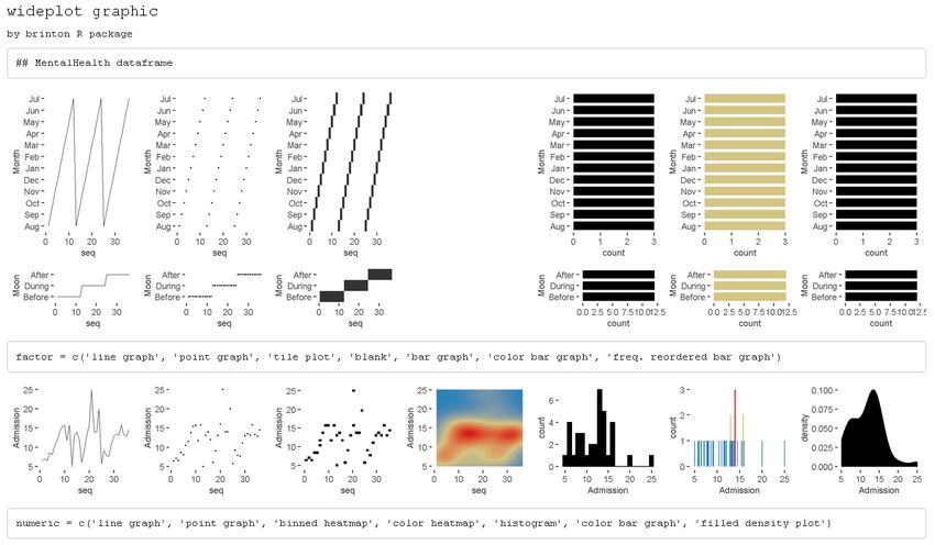
C ONTRIBUTED RESEARCH ARTICLE                                                                                                     323

          This can also be achieved with the patchwork package (Pedersen, 2019) that adds versatility to the
          composition of multipanel graphics by introducing operators that partition the canvas.
              A second type of multipanel graphic is the conditioning plot1 . In these, the same graphic type is
          repeated in different panels at the same scale, representing subsets of data according to the level of
          one or more variables. A third type of multipanel graphic is the matrix of plots, which links pairs
          of variables of the same type and from the same dataset. A classic example is the scatterplot matrix
          (Hartigan, 1975), or, more recently, the HE plot (Friendly, 2007). The diagonal of these grids can be
          populated with a different graphic type, since a single variable is involved. A variant of the matrix of
          plots uses source variables of different types that, when paired, result in a grid with multiple graphic
          types, depending on how the variables are combined. This graphic type is known as a generalized
          pairs plot (Emerson et al., 2013).

          The brinton package

          We created brinton package to facilitate exploratory data analysis following the visual information-
          seeking mantra (Shneiderman, 1996): “Overview first, zoom and filter, then details on demand.”
          The main idea is to assist the user during these three phases through three functions: wideplot(),
          longplot() and plotup(). A distinctive feature is the following: the wideplot() function provides a
          limited selection of available graphics for all the variables in a data frame, the longplot() function
          provides all the range of available graphics for a limited selection of variables and, finally, the plotup()
          function provides one single graphic for a limited selection of variables. While each of these functions
          has its own arguments and purpose, all three serve to facilitate exploratory data analysis and the
          selection of a suitable graphic.
              The wideplot() function allows the user to explore a dataset as a whole using a grid of graphics
          in which each variable is represented through multiple graphics. Once we have explored the dataset
          as a whole, the longplot() allows us to explore other graphics for a given variable. This function
          also presents a grid of graphics, but instead of showing a selection of graphics for each variable, it
          presents the full range of graphics available in the package to represent a single variable. Once we
          have narrowed in on a certain graphic, we can use the plotup() function, which presents the values of
          a variable on a single graphic. We can access the code of the resulting graphic and adapt it as needed.
          These three functions expand the graphic types that are presented automatically by the autoGEDA
          packages in the R environment.
             brinton package is based primarily in the grammar of graphics (Wilkinson, 2005) implemented in
          R by the package ggplot2. Additionally, it draws on the package gridExtra (Auguie, 2017) for creating
          multipanel graphics and on rmarkdown (Allaire et al., 2019) for dynamically composing the results.
              In the context of graphics packages in R based on the grid system, the package lattice allows the
          user to create a range of some 13 graphic types, which can be adapted to a very fine level of detail.
          ggplot2 makes it possible to control even the finest detail of a graphic, but this comes at the price of
          learning its grammar and its layer system. In contrast, brinton package makes it possible for the user
          to select statistical graphics by name from a wide range of available graphics and, if he or she knows
          the grammar of ggplot2, adapt them as needed. To create a statistical graphic in R, if the desired
          graphic is already implemented in brinton package, the user must simply specify the data source and
          the graphic type to be produced.
              The package can be installed easily from the Comprehensive R Archive Network (CRAN) using
          the R console. When the package is loaded into memory, it provides a startup message that pays
          homage to Henry D. Hubbard’s enthusiastic introduction to the book Graphic Presentation (Brinton,
          1939):
            install.packages("brinton")
            library(brinton)
            M a G i C i N G R a P H S

          The wideplot function

          When a dataset is loaded into R, the next function to be used tends to be str(). This occurs because
          if we don’t determine the nature of the values explicitly, the functions for loading datasets make
             1 The terminology for conditioning plots is not unanimous. These plots were first described by J. Bertin as séries

          homogènes (Bertin, 1967, p.26). Later, E. Tufte introduced them as small multiples (Tufte, 1983). W.S. Cleveland
          called them juxtaposed panels (Cleveland, 1985, p.200) and also trellis graphics (Becker et al., 1996). In the R
          environment they are generally known as lattice graphics (Sarkar, 2008) or facet plots, based on the description of
          this technique by L. Wilkinson (2005) and later implemented in ggplot2

          The R Journal Vol. 12/2, December 2020                                                           ISSN 2073-4859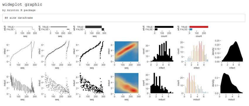
C ONTRIBUTED RESEARCH ARTICLE                                                                                        324

          assumptions about it. The function str() shows in the console the type of object to which the function
          is being applied, the number of rows, the number and names of columns, their class (number, factor,
          etc.) and the initial observations for each variable. The wideplot() function takes inspiration from
          this function, but instead of describing the dataset in textual or tabular form, it does it graphically.
          We can easily compare the results of these two functions, for example, with the dataset esoph from
          a case-control study of esophageal cancer in Ille-et-Vilaine, France. The dataset has three ordered
          factor-type variables and two numerical variables:

            str(esoph)

          #> 'data.frame':    88 obs. of 5 variables:
          #> $ agegp     : Ord.factor w/ 6 levels "25-34"   factor = NULL, character = NULL, datetime = NULL, numeric = NULL,
          #>   group = NULL, ncol = 7, label = 'FALSE')

             The only argument necessary to obtain a result is data that expects a data.frame class
          object; dataclass selects and sorts the types of variables to be shown; ncol filters the first n
          columns of the grid, between 3 and 7, which will be shown. The fewer columns displayed,
          the larger the size of the resulting graphics, a feature that is especially useful if the scale

          The R Journal Vol. 12/2, December 2020                                               ISSN 2073-4859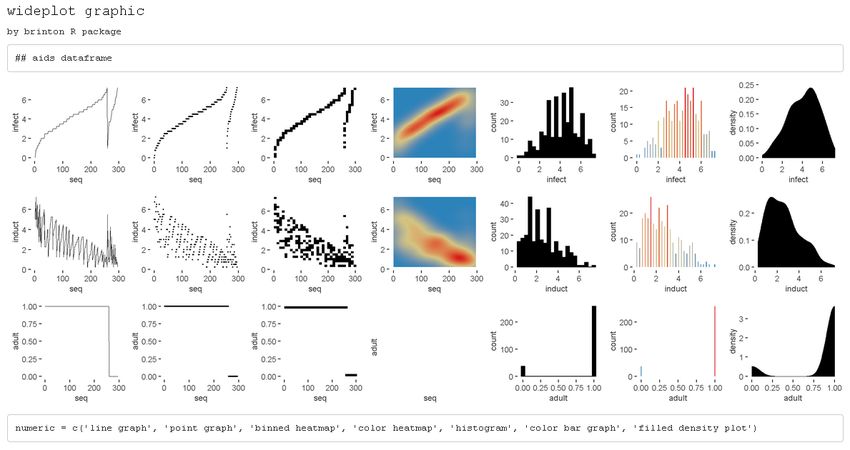
C ONTRIBUTED RESEARCH ARTICLE                                                                                325

          labels dwarf the graphics area; label adds to the grid a vector below each group of rows
          according to the variable type, with the names and order of the graphics; logical, ordered,
          factor, character, datetime and numeric make it possible to choose which graphics, from
          among the ones included by the specimen (Sec. 2.3.4), appear in the grid and in what order,
          for each variable type. Finally, group changes the selection of graphics that are shown by
          default according to the criteria of Table 1.
              If the order and graphic types to be shown for each variable type are not specified and
          if the graphic types aren’t filtered using the argument group, then the default graphic will
          contain an opinion-based selection of graphics for each variable type, organized especially
          to facilitate comparison between graphics of the same row and between graphics of the same
          column. The user can overwrite this selection of graphics as needed, using the arguments
          logical, ordered, factor, character, datetime and numeric.

           group        graphic type
           sequence     includes the sequence in which the values are observed so that an axis
                        develops this sequence. e.g. line graph, point-to-point graph
           scatter      marks represent individual observations. e.g. point graph, stripe graph
           bin          marks represent aggregated observations based on class intervals.
                        e.g. histogram, bar graph
           model        represents models based on observations. e.g. density plot, violin plot
           symbol       represents models based on observations. and not only points, lines or areas
                        e.g. box plot
           GOF          represents the goodness of fit of some values with respect to a model
                        e.g. qq plot
           random       chosen at random

                      Table 1: Possible values for the group argument of the wideplot() function.

          The longplot function

          To facilitate economy of calculation, the wideplot() function presents a limited number of
          graphics in each row. If the user wants to expand the range of suggested graphics for a
          given variable, he or she should use the longplot function, which returns a grid with all of
          the graphics considered by the package (See Figure 2) for that variable. The structure of the
          function is very simple longplot(data,vars,label = TRUE) and we can easily check the
          outcome of applying this function to the variable alcgp of the dataset esoph:

            longplot(data = esoph, vars = "alcgp")

          The R Journal Vol. 12/2, December 2020                                            ISSN 2073-4859
C ONTRIBUTED RESEARCH ARTICLE 326
Figure 2: Output of longplot(esoph, ’alcgp’). A grid of graphics where the variable alcgp in the
dataset esoph is displayed for the full range of graphics considered by the package.
We named the resulting graphic type longplot because it shows the full range of available
graphics to represent the relationships among the values of a limited selection of variables
(although for now, in this package we have only included graphics for a single variable).
The arguments of the function are data, which must be a data.frame class object; vars,
which requires the name of a specific variable of the dataset; and label, which does not
have to be defined and which adds a vector below each row of the grid indicating the name
of each graphic. Unlike the grid of the wideplot function, the grid of the longplot function
does not include parameters to limit the range of graphics to be presented. We made this
decision because the main advantage of this function is precisely that it presents all of the
graphic representations available for a given variable. However, we do not rule out adding
filters that limit the number of graphics to be shown if this feature seems useful as the
catalog fills with graphics. Each graphic presented can be called explicitly by name using
the functions wideplot() and plotup(), which is why the argument label has been set to
TRUE by default in this case.
The range of graphics that the longplot() function returns is sorted so that in the rows
we find different graphic types and in the columns different variations of the same graphic
type. This organization, however, is not absolute and in some cases in order to compress the
results, we find different graphic types in the same row.
The plotup function
The plotup() function has the following structure: plotup(data,vars,diagram,output =
'plots pane'). By default, this function returns an object belonging to class gg and ggplot
whose graphic can be rendered in the plots pane of RStudio. This graphic is based on a
variable from a given dataset and the name of the desired graphic, from among the names
included by the specimen that we present in the next subsection. We can easily check the
outcome of applying this function to produce a line graph from the variable ncases of the
dataset esoph (See Figure 3) :
plotup(data = esoph, vars = 'ncases', diagram = 'line graph', output = 'html')
The R Journal Vol. 12/2, December 2020 ISSN 2073-4859C ONTRIBUTED RESEARCH ARTICLE 327
Figure 3: Output of plotup(esoph, ’ncases’, ’line graph’). A line graph from the variable ncases
in the dataset esoph.
This function requires three arguments: data, vars and diagram. The fourth argument,
output, is optional and has the default value of plots pane. However, if is set to it html or
console, instead of returning a c("gg","ggplot") object, the function cause a side-effect:
either creating and displaying a temporary html file, or printing the ggplot2 code to the
console. This feature is especially useful to adapt the default graphic to the specific needs
and preferences of the user.
The diagram argument accepts any of the values admitted by the logical, ordered,
factor, character, datetime and numeric arguments of the wideplot() function. These
values coincide with the names of the graphics considered by the package and included in
the specimen. The naming convention of these graphs is implicitly addressed in Section 4
“Graphical degrees of freedom”.
plotup(data = esoph, vars = 'ncases', diagram = 'line graph',
output = 'console')
#> ggplot(esoph, aes(x=seq_along(ncases), y=ncases)) +
#> geom_line() +
#> labs(x='seq') +
#> theme_minimal() +
#> theme(panel.grid = element_line(colour = NA),
#> axis.ticks = element_line(color = 'black'))
The specimen
The documentation of the package includes the vignette “1v specimen”, which contains a
specimen with images of all the graphic types for a single variable, incorporated into the
package according to the variable type. These graphics serve as an example so that the user
can rapidly check whether a graphic has been incorporated, the type or types of variable
for which it has been incorporated, and the label with which it has been identified. The
suitability of a particular graphic will depend on the datasets of interest and the variables
of each particular user. We have incorporated this specimen in its current version as
supplementary material.
Graphical degrees of freedom
The utility of this package is based on the fact that different graphical representations of the
same data make it possible not only to observe different characteristics of the data, but also
to show a certain characteristic more effectively. For this reason, the graphics considered by
this package enjoy a large number of graphical degrees of freedom. This makes it possible
for the catalog to include both commonly used graphics and graphics that have not yet been
developed. The concept of graphical degrees of freedom has been used by Benger and Hege
The R Journal Vol. 12/2, December 2020 ISSN 2073-4859C ONTRIBUTED RESEARCH ARTICLE 328
(2006) to refer to Bertin’s visual variables (1967, p.43) but with some modifications. Here we
use the concept in a broader sense, as detailed below.
• Type of graphic. The main degree of freedom of the graphics catalog is the graphic
type. The different graphic types are not necessarily ones that differ greatly from each
other. To the contrary, very similar graphics coexist because a high number of users
prefer each of them. This is the case, for example, of the density plot and the violin
plot shown in Figure 4.
wideplot(data = esoph[5],
numeric = c('filled violin plot', 'filled density plot'))
Figure 4: 1st degree of freedom (type of graphic). Density and violin plots of variable ncontrols (in
the dataset esoph).
• Chromatic scales. The same graphic can have different versions depending on the
chromatic scale associated with a variable in the data or computed from it. We can see
an example of this in the following figure 5. Despite the fact that color can be broken
down into the three visual variables of hue, saturation and value, for the purposes of
this package we have only taken into account hue in the case of the color scale and
value in the case of the grayscale, following Bertin’s classification of visual variables
(1967, p.43).
wideplot(data = esoph[5],
numeric = c('histogram', 'bw histogram', 'color histogram'))
Figure 5: 2nd degree of freedom (chromatic scale). Plots of variable ncontrols (in the dataset esoph)
with different chromatic scales.
• Agreggation method: scattered or binned. The same values can be represented such
that each mark represents either a single value or an aggregate value. An example of
this feature can be observed in Figure 6.
wideplot(data = esoph[5],
numeric = c('stripe graph', 'binned stripe graph', 'bar graph',
'histogram'))
The R Journal Vol. 12/2, December 2020 ISSN 2073-4859C ONTRIBUTED RESEARCH ARTICLE 329
Figure 6: 3rd degree of freedom (aggregation method). Plots of variable ncontrols (in the dataset
esoph) with single or aggregate values.
• Nested panels. One possibility (which has been little explored) is that of subdividing
into different panels the cells of the multipanel graphic, to create systems of coordinates
inside systems of coordinates. This solution is similar to the treemap. In the example
in Figure 7, the graphic on the right has three panels that can substitute the first three
graphics.
wideplot(data = esoph[5],
numeric = c('violin plot', 'stripe graph', 'box plot', '3 uniaxial'))
Figure 7: 4th degree of freedom (nested panels). Plots of variable ncontrols (in the dataset esoph)
with single and multiple panels (the first three ones and the last one respectively).
• Shape. The same information can be represented with marks of different shapes.
This possibility is exemplified in Figure 8, which compares two graphics with similar
composition but different marks: circular or square.
wideplot(data = esoph[5],
numeric = c('color binned point graph', 'color binned heatmap'))
Figure 8: 5th degree of freedom (shape). Plots of variable ncontrols (in the dataset esoph) with marks
of different shapes.
• Implantation. The same values can be represented with marks of a different type of
implantation, such as a point, a line, an area or a combination of these. For example,
Figure 9 compares a point graph, a line graph, and a point-to-point graph.
wideplot(data = esoph[5],
numeric = c('point graph', 'line graph', 'point-to-point graph'))
The R Journal Vol. 12/2, December 2020 ISSN 2073-4859C ONTRIBUTED RESEARCH ARTICLE 330
Figure 9: 6th degree of freedom (implantation). Plots of variable ncontrols (in the dataset esoph) with
marks of a different type of implantation.
• Transition. The transition or itinerary between two points can help reflect the discrete
nature of the changes in the values observed. Figure 10 compares two line graphs with
different transitions between points.
wideplot(data = esoph[5],
numeric = c('line graph', 'stepped line graph'))
Figure 10: 7th degree of freedom (transition). Plots of variable ncontrols (in the dataset esoph) with
different transitions between points.
• Collation. The values of variables, especially those that aren’t related to order, can be
sorted according to different criteria. This package, as shown in Figure 11 uses three:
the order of appearance in the sequence of observations, the frequency with which the
values are observed and alphabetical order.
wideplot(data = data.frame('Region' = state.region),
factor = c('tile plot',
'freq. reordered tile plot',
'alphab. reordered tile plot'))
Figure 11: 8th degree of freedom (collation). Plots of variable Region with the values sorted according
to different criteria.
• Superposition. The final degree of freedom that we consider is the possibility of
including graphics that superpose marks whose data source is the same but that have
different degrees of transformation (see Figure 12).
wideplot(data = esoph[5],
numeric = c('color point graph',
'color point graph with trend line'))
The R Journal Vol. 12/2, December 2020 ISSN 2073-4859C ONTRIBUTED RESEARCH ARTICLE 331
Figure 12: 9th degree of freedom (superposition). Plots of variable ncontrols (in the dataset esoph)
with and without the superposition of a trend line.
To construct the specimen we have ruled out some degrees of freedom, for example, the
group of imposition (Bertin, 1967, p.52) and the permutation of spacial variables (Bertin, 1967,
p.43). In other words, brinton package exclusively presents diagrams and not networks
or maps, nor does it show alternatives whose only difference is that the x and y axes are
switched.
Application to real datasets
The main application of a package for exploratory data analysis is to help the user make
sense of the data. This includes describing the number and nature of the variables, the
number of observations and examples of the variables–this is precisely what the str()
function does. It also includes evaluating the validity and quality of the data and the
properties of the values found.
We can deduce the number of variables from the number of rows in the grid of the
wideplot graphic. The names of the variables are found in each of the graphics that the
catalog now contains. We can determine the variables’ nature–in terms of the measurement
scale—-by observing the range of graphics selected and specifying the value label = TRUE
for the grids of wideplot and longplot graphics. We can discern the number of observations
by examining the graphics that include the sequence of observations or, in the case of
categorical variables, by counting the categories and the number of observations for each
one. Wideplot graphics, in contrast to the textual summary of the str() function, show
examples not only of the first observations but of all observations. To evaluate the validity of
the data, we can observe specific graphics that allow us to identify outliers, missing values
or discontinuity in the observations. The same goes for the properties of the values found.
There is a huge range of graphics, each of which makes it possible to highlight different
properties. Below we list a series of tasks for which the functions included in brinton are
useful, and describe the process for carrying them out.
Identify multi-column sorting
Here we describe how to use the wideplot() function to determine whether the observations
of the dataset aids of the package KMsurv are sorted according to one of the variables. This
dataset has three variables, infect (infection time for AIDS in years), induct (induction
time for AIDS in years), and adult (indicator of adult: 1=adult, 0=child). To accomplish the
task, we first install the package, then load it into memory and run the wideplot function
with its default output.
install.packages('KMsurv')
data(aids, package = 'KMsurv')
wideplot(data = aids, label = TRUE)
The R Journal Vol. 12/2, December 2020 ISSN 2073-4859C ONTRIBUTED RESEARCH ARTICLE 332
Figure 13: A grid of graphics generated by wideplot(aids, label = T). Each row corresponds to a
variable in the dataset aids. The line graph shows that the dataset is sorted first by the variable adult
and then by the variable infect.
From the result in Figure 13, we observe that the line graph is the one that best shows
that the dataset is sorted first by the variable adult and then by the variable infect. To
finish selecting the most suitable graphic we can then execute the same function but limit
the graphic types such that only two variations of line graph are shown. We can moreover
limit the function so that it displays, for example, only five columns, so that the graphics
will be larger.
wideplot(data = aids,
numeric = c('line graph', 'stepped line graph'), ncol = 5)
Figure 14: A grid of graphics generated by wideplot(aids, numeric = c(’line graph’, ’stepped
line graph’), ncol=5). Each row corresponds to a variable in the dataset aids. Graphic types are
limited to line and stepped line types.
The result is two variations of the line graph for each variable, in which we can clearly
see that the data set is sorted first by the variable adult and then by the variable infect. In
this case, there may be equally valid arguments for using the graphics of the first column as
the graphics of the second column.
The R Journal Vol. 12/2, December 2020 ISSN 2073-4859C ONTRIBUTED RESEARCH ARTICLE 333
This same example also works for datasets with categorical variables, such as the
dataset MentalHealth of the package Stat2Data. This dataset consists of three variables:
Month (month of the year); Moon (relationship to full moon: After, Before, or During); and
Admission (number of emergency room admissions). The first two variables are categorical
and the third is numerical. If we examine the line graph and also the tile plot for the factor-
type variables and the binned heatmap graphic for the numerical variables, we can easily
see that the dataset is sorted by the variable Moon and then by the variable Month (see Figure
15).
install.packages('Stat2Data')
data(MentalHealth, package = 'Stat2Data')
wideplot(data = MentalHealth, label = TRUE)
Figure 15: A grid of graphics generated by wideplot(MentalHealth, label = T). Each row cor-
responds to a variable in the dataset MentalHealth. It is observed that the dataset is sorted by the
variable Moon and then by the variable Month.
Identify variables that can be reclassified
When loading a dataset it is important to check which assumptions the function has made
and which variables can be reclassified. We can see an example of this in Figure 14, which
shows that the variable adult of the dataset aids is better treated as a logical-type variable
than an integer. If we recode the variable type more appropriately, when we apply the
wideplot() function again, the graphics also tend to be more appropriate. In Figure 16 we
see the result after the variable adult is reclassified.
aids$adultC ONTRIBUTED RESEARCH ARTICLE 334
Figure 16: A grid of graphics generated by wideplot(aids). Each row corresponds to a variable in
the dataset aids. The variable adult has been reclassified from integer to logical in order to obtain
more appropriate graphics.
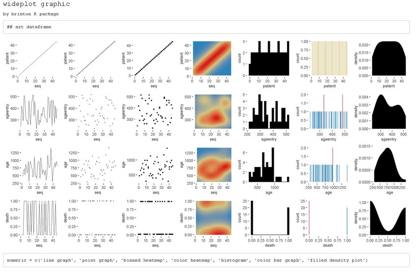
Identify key variables
The best way to identify key variables is by using complementary graphics. Figure 17 makes
it possible, for example, to identify rapidly the variable patient of the dataset azt in the
package KMsurv, as a key variable, given that it assigns a sequential number to each record,
each of which is observed a single time. We can draw these two conclusions from the line
graph and the color bar graph.
data(azt, package = 'KMsurv')
wideplot(data = azt, label = TRUE)
Figure 17: A grid of graphics generated by wideplot(azt, label=TRUE). Each row corresponds to a
variable in the dataset azt. The line graph and the color bar graph recognize the variable patient as a
key variable that assigns a sequential number to each record.
In the case of categorical key variables, the same line graph and color bar graph would
also help us to identify the key variable. Figure 18 shows these two graphs for the factor-type
variable of the dataset SpeciesArea in the package Stat2Data, which allow us to identify
rapidly the variable Name as a key variable.
data(SpeciesArea, package = 'Stat2Data')
The R Journal Vol. 12/2, December 2020 ISSN 2073-4859C ONTRIBUTED RESEARCH ARTICLE 335
wideplot(data = SpeciesArea, dataclas = c('factor'),
factor = c('line graph', 'color bar graph'), ncol = 5)
Figure 18: Line and color bar graphs of the factor-type variable Name (in the dataset SpeciesArea)
produced by the function wideplot(). It is observed that the variable Name is a key variable since the
values are not repeated and observed once.
Be surprised by serendipity
Next we describe isolated cases in which we are surprised by the values that the data depict.
We use the following procedure to locate unexpected aspects of the data: first we obtain
a general view of the dataset using the function wideplot(); next we focus our attention
on one variable in particular and explore all of the compatible graphics using the function
longplot(); finally, we use the function plotup() to obtain the graphic that best enables us
to identify, narrow down and communicate the aspect of the data that we have found.
• The first example of an unexpected funding appears in the variable experience (years
of potential work experience) of the dataset HI in the package Ecdat. This dataset
contains 22,272 records of 13 variables that link health insurance policies to the weekly
hours worked by the wives of the policyholders, while the variable experience refers
to the years of potential work experience of the wives. If we look at the bar graph
applied to this numerical variable (see Figure 19), we see that the frequency of the
whole values is systematically greater than the frequency of the real non-whole values.
This behavior could indicate that the variable can be informed with high precision
and whoever informed the variable experience tended to round to the unit. Another
possibility is that the dataset was constructed by joining two data sources with different
degrees of precision2
data(HI, package = 'Ecdat')
HI_samC ONTRIBUTED RESEARCH ARTICLE 336
• In the same dataset we can see that we could reach mistaken conclusions about the
distribution of the variable husby (husband’s income in thousands of dollars) if we
only looked at a histogram. As we can see in Figure 20, the distribution, and in
particular the value zero, acquires a different value if we compare the histogram (left)
with another graphic that isn’t as common for numerical variables: the bar graph
(right), which shows the count of unique values. The bar graph makes it possible to
clearly differentiate two groups: the informants whose husbands have no income and
the informants whose husbands do have income (and to whom, therefore, it makes
more sense to ask approximate income).
library(patchwork)
plotup(HI_sam, 'husby', 'histogram') + plotup(HI_sam, 'husby', 'bar graph')
Figure 20: Histogram (left) and bar plot (right) of the variable husby (in the dataset HI_sam) produced
by the function plotup(). The bar plot makes it possible to identify the zero as a value with a special
meaning.
Combine graphics that best explains a specific data characteristic
Just as multipanel graphics make it possible to reveal different aspects of the data, it can also
be helpful to use a selection of graphics to present a certain characteristic of the data. Next,
we show an example of how brinton package can help us improve the default graphics in
order to combine them later to show a particular feature.
• A recurring problem when we deal with datasets with many records is that when
marks overlap, we cannot correctly interpret the set of observations. The presentation
of multiple graphics to represent the same values enables us to identify these overlaps
and improve the representation that the package shows by default. For example,
in Figure 21 we can see how the point graph for the same variable husby is unclear
because the marks overlap.
plotup(data = HI_sam, vars = 'husby', diagram = 'point graph')
Figure 21: Point plot of the variable husby (in the dataset HI_sam) produced by the function plotup().
The point plot does not identify the zero as a value with a special meaning because the marks overlap.
• We do not have to accept the default result. Rather we can retrieve the package’s
ggplot2 function using the argument output = 'console' and then improve it:
The R Journal Vol. 12/2, December 2020 ISSN 2073-4859C ONTRIBUTED RESEARCH ARTICLE 337
plotup(data = HI_sam, vars = 'husby', diagram = 'point graph',
output = 'console')
#> ggplot(HI_sam, aes(x=seq_along(husby), y=husby)) +
#> geom_point() +
#> labs(x='seq') +
#> theme_minimal() +
#> theme(panel.grid = element_line(colour = NA),
#> axis.ticks = element_line(color = 'black'))
• In this case we can, for example, improve the graphic by reducing the size of the points
and adding an alpha channel (see Figure 22).
newpointgraphC ONTRIBUTED RESEARCH ARTICLE 338
Figure 23: Multipanel graphic as a composition of three plots of the variable husby (in the dataset
HI_sam). The source of each plot is the function plotup(). Combining the three plots helps to highlight
different aspects of the distribution of the variable husby.
The resulting multipanel graphic shows that throughout the dataset, the revenue distri-
bution remains essentially constant, highlighting the number of husbands without income
and rounding the reported values to nice numbers such as 25, 30, 40, 50 and 100–although in
reality, the value that draws a horizontal line around 100 is, surprisingly, 99,999. And here
we have another mystery to solve.
Conclusions
We have introduced brinton package, a graphical EDA tool designed to facilitate the presen-
tation, selection and editing of statistical graphics built on ggplot2. This package maximizes
the deterministic strategy of graphic selection by presenting a range of graphics that a user
can choose by name, automating the construction of graphics and even allowing the user to
recover the underlying ggplot2 function in order to adapt the graphics as necessary. This
package makes it easier for a user to become familiar with a dataset and generate hypotheses
based on it.
This is a project in progress and new software implementations are being updated and
released. We plan to create a fuller catalog that will include graphics that can combine up to
three variables, improve the aesthetics of the default graphics and add new functions for
autoGEDA.
Acknowledgements
We thank Michael Friendly and Pedro Valero-Mora for corresponding with AUTHOR 1
about the package cowplot, which inspired the wideplot() function that forms the core of
this package. We acknowledge Susan Frekko for translating so accurately the manuscript
from Catalan.
Bibliography
J. Allaire, Y. Xie, J. McPherson, J. Luraschi, K. Ushey, A. Atkins, H. Wickham, J. Cheng,
W. Chang, and R. Iannone. rmarkdown: Dynamic Documents for R, 2019. URL https:
//rmarkdown.rstudio.com. R package version 1.12. [p323]
B. Auguie. gridExtra: Miscellaneous Functions for "Grid" Graphics, 2017. URL https://CRAN.R-
project.org/package=gridExtra. R package version 2.3. [p321, 323]
R. A. Becker, W. S. Cleveland, and M.-J. Shyu. The visual design and control of trellis display.
Journal of computational and Graphical Statistics, 5(2):123–155, 1996. [p323]
W. Benger and H.-C. Hege. Strategies for direct visualization of second-rank tensor fields.
In J. Weickert and H. Hagen, editors, Visualization and Processing of Tensor Fields, pages 191–
214. Springer Berlin Heidelberg, Berlin, Heidelberg, 2006. ISBN 978-3-540-31272-7. doi:
10.1007/3-540-31272-2_11. URL https://doi.org/10.1007/3-540-31272-2_11. [p328]
The R Journal Vol. 12/2, December 2020 ISSN 2073-4859C ONTRIBUTED RESEARCH ARTICLE 339
J. Bertin. Sémiologie graphique. Les diagrammes, les réseaux, les cartes. Mouton, Paris, 1967.
[p323, 328, 331]
J. Bertin. La graphique et le traitement graphique de l’information. Flammarion, Paris, 1977.
[p321]
W. Brinton. Graphic Presentation. McGraw-Hill Book Company Inc., New York City, 1939.
URL https://archive.org/details/graphicpresentat00brinrich. [p322, 323]
W. Chang and B. Borges Ribeiro. shinydashboard: Create Dashboards with ’Shiny’, 2018. URL
https://CRAN.R-project.org/package=shinydashboard. R package version 0.7.1. [p322]
W. Cleveland. The Elements of Graphing Data. Hobart Press, Summit, New Jersey, 1985. [p323]
D. Comtois. summarytools: Tools to Quickly and Neatly Summarize Data, 2019. URL https:
//CRAN.R-project.org/package=summarytools. R package version 0.9.3. [p322]
D. Cook, D. F. Swayne, and A. Buja. Interactive and dynamic graphics for data analysis: with R
and GGobi. Springer Science & Business Media, 2007. [p321]
B. Cui. DataExplorer: Automate Data Exploration and Treatment, 2019. URL https://CRAN.R-
project.org/package=DataExplorer. R package version 0.8.0. [p322]
Dayanand Ubrangala, K. R, R. Prasad Kondapalli, and S. Putatunda. SmartEDA: Summarize
and Explore the Data, 2019. URL https://CRAN.R-project.org/package=SmartEDA. R
package version 0.3.2. [p322]
J. W. Emerson, W. A. Green, B. Schloerke, J. Crowley, D. Cook, H. Hofmann, and H. Wickham.
The generalized pairs plot. Journal of Computational and Graphical Statistics, 22(1):79–91,
2013. doi: 10.1080/10618600.2012.694762. URL https://doi.org/10.1080/10618600.
2012.694762. [p323]
M. Friendly. He plots for multivariate general linear models. Journal of Computational and
Graphical Statistics, 16(4):421–444, 2007. [p323]
M. Friendly. Lecture 2: Standard graphics in r, 2018. URL http://www.datavis.ca/courses/
RGraphics/. OpenCourseWare. [p321]
J. A. Hartigan. Printer graphics for clustering. Journal of Statistical Computation and Simulation,
4(3):187–213, 1975. [p323]
R. Iannone, J. Allaire, and B. Borges. flexdashboard: R Markdown Format for Flexible Dashboards,
2018. URL https://CRAN.R-project.org/package=flexdashboard. R package version
0.5.1.1. [p322]
T. Kamps. Diagram Design: A Constructive Theory. Springer Berlin Heidelberg, 1999. [p321]
P. Millán-Martínez and P. Valero-Mora. Automating statistical diagrammatic representations
with data characterization. Information Visualization, 17(4):316–334, 2018. [p321]
R. L. Oliver. Effect of expectation and disconfirmation on postexposure product evaluations:
An alternative interpretation. Journal of applied psychology, 62(4):480, 1977. [p321]
T. L. Pedersen. patchwork: The Composer of Plots, 2019. URL https://CRAN.R-project.org/
package=patchwork. R package version 1.0.0. [p323]
A. H. Petersen and C. T. Ekstrøm. dataMaid: Your assistant for documenting supervised
data quality screening in R. Journal of Statistical Software, 90(6):1–38, 2019. doi: 10.18637/
jss.v090.i06. [p322]
R Core Team. R: A Language and Environment for Statistical Computing. R Foundation for
Statistical Computing, Vienna, Austria, 2018. URL https://www.R-project.org/. [p]
The R Journal Vol. 12/2, December 2020 ISSN 2073-4859C ONTRIBUTED RESEARCH ARTICLE 340
R. Rao and S. K. Card. The table lens: Merging graphical and symbolic representations
in an interactive focus + context visualization for tabular information. In Proceedings of
the SIGCHI Conference on Human Factors in Computing Systems, CHI ’94, pages 318–322,
New York, NY, USA, 1994. ACM. ISBN 0-89791-650-6. doi: 10.1145/191666.191776. URL
http://doi.acm.org/10.1145/191666.191776. [p322]
A. Rushworth. inspectdf: Inspection, Comparison and Visualisation of Data Frames, 2019. URL
https://CRAN.R-project.org/package=inspectdf. R package version 0.0.4. [p322]
D. Sarkar. Lattice: Multivariate Data Visualization with R. Springer, New York, 2008. URL
http://lmdvr.r-forge.r-project.org. ISBN 978-0-387-75968-5. [p321, 323]
P. Seibelt. xray: X Ray Vision on your Datasets, 2017. URL https://CRAN.R-project.org/
package=xray. R package version 0.2. [p322]
B. Shneiderman. The eyes have it: a task by data type taxonomy for information visualiza-
tions. In Proceedings 1996 IEEE Symposium on Visual Languages, pages 336–343, Sep. 1996.
doi: 10.1109/VL.1996.545307. [p323]
M. Staniak and P. Biecek. The landscape of r packages for automated exploratory data
analysis. arXiv preprint arXiv:1904.02101, 2019. [p321, 322]
M. Tennekes, E. de Jonge, P. J. Daas, et al. Visualizing and inspecting large datasets with
tableplots. Journal of Data Science, 11(1):43–58, 2013. [p322]
T. M. Therneau. A Package for Survival Analysis in S, 2015. URL https://CRAN.R-project.
org/package=survival. version 2.38. [p321]
M. Theus and S. Urbanek. Interactive Graphics for Data Analysis: Principles and Examples
(Computer Science and Data Analysis). Chapman & Hall/CRC, 2008. ISBN 1584885947,
9781584885948. [p321]
N. Tierney. visdat: Visualising whole data frames. JOSS, 2(16):355, 2017. doi: 10.21105/joss.
00355. URL http://dx.doi.org/10.21105/joss.00355. [p322]
E. R. Tufte. The Visual Display of Quantitative Information. Graphics Press, Cheshire, 1983.
[p323]
J. Tukey. Exploratory Data Analysis. Addison-Wesley series in behavioral science. Addison-
Wesley Publishing Company, 1977. ISBN 9780201076165. URL https://books.google.
es/books?id=UT9dAAAAIAAJ. [p321]
H. Wickham. ggplot2: Elegant Graphics for Data Analysis. Springer-Verlag New York, 2016.
ISBN 978-3-319-24277-4. URL http://ggplot2.org. [p321]
C. O. Wilke. cowplot: Streamlined Plot Theme and Plot Annotations for ’ggplot2’, 2019. URL
https://CRAN.R-project.org/package=cowplot. R package version 1.0.0. [p322]
L. Wilkinson. The Grammar of Graphics. Statistics and Computing. Springer, 2nd edition,
2005. [p323]
Pere Millán-Martínez
Servei Català de Trànsit
Carrer Diputació, 355 08009 Barcelona, Spain
Research Group on Methodology, Methods, Models and Outcomes of Health and Social Sciences
(M3 O)
Faculty of Health and Welfare Sciences
Universitat de Vic - UCC
Sagrada Família, 7 08500 Vic, Spain
ORCID: 0000-0003-0879-9358
info@sciencegraph.org
The R Journal Vol. 12/2, December 2020 ISSN 2073-4859C ONTRIBUTED RESEARCH ARTICLE 341
Ramon Oller
Data Analysis and Modeling Research Group
Departament d’Economia i Empresa
Universitat de Vic - UCC
Sagrada Família 7, 08500 Vic, Spain
ORCID: 0000-0002-4333-0021
ramon.oller@uvic.cat
The R Journal Vol. 12/2, December 2020 ISSN 2073-4859You can also read