Remote Sensing of Environment - ORBi
←
→
Page content transcription
If your browser does not render page correctly, please read the page content below
Remote Sensing of Environment 253 (2021) 112229
Contents lists available at ScienceDirect
Remote Sensing of Environment
journal homepage: www.elsevier.com/locate/rse
Detection of shadows in high spatial resolution ocean satellite data
using DINEOF
Aida Alvera-Azcárate a, *, Dimitry Van der Zande b, Alexander Barth a,
João Felipe Cardoso dos Santos b, Charles Troupin a, Jean-Marie Beckers a
a
AGO-GHER, University of Liège Allée du Six Aout, 17, Sart Tilman, Liège 4000, Belgium
b
Royal Belgian Institute of Natural Sciences (RBINS), Direction Natural Environment Rue Vautier 29, 1000 Brussels, Belgium
A B S T R A C T
Cloud shadows present in high spatial resolution remote sensing datasets can affect the quality of the data if they are not properly detected and removed. When
working with ocean data, cloud shadows are often difficult to differentiate from non-shadow values, since they show similar spectral characteristics than water pixels.
A methodology to detect cloud shadows over the ocean is proposed. The present approach combines a series of tests applied directly to the physical variables derived
from the satellite measured radiances, and it therefore does not depend on the wavebands measured by a specific satellite sensor. The tests include a departure from
an EOF basis calculated using DINEOF, a threshold test, a proximity to cloud test and a ray tracing test. The weighing of the different tests can be adapted to each case
or domain of study. The results are compared to manually detected shadows and to another shadow detection method. The approach works with cloud shadows of all
sizes, and also with very small objects shadows, like the shadows projected by offshore windmills.
1. Introduction can cast also small shadows. The shadows from clouds and these objects
do not show specific spectral characteristics over water pixels (i.e. the
The Multispectral Instrument (MSI) onboard Sentinel-2 satellites A ocean, which is in general a dark surface), which is precisely the object
and B is mainly designed to provide information on land surfaces for of this study. The intensity of the cloud shadows depends on the thick
applications in agriculture, geology, forestry, mapping, global change ness of the originating cloud. This makes it very difficult to accurately
research, etc. However, its performance in terms of signal-to-noise ratio detect and flag them in order to exclude them from further processing.
(SNR) is sufficient to be used for marine applications, especially in Furthermore, it is difficult to know the altitude of the different clouds
turbid coastal waters. Compared to the dedicated ocean colour sensors present in a Sentinel-2 satellite image, an information that would allow
(Moderate Resolution Imaging Spectroradiometer-Aqua -MODIS-AQUA- the location of the shadows by projection. In addition, if a cloud is out of
, Visible Infrared Imaging Radiometer Suite -VIIRS- and Sentinel-3 the limits of the domain of study, but projecting a shadow within it,
Ocean and Land Colour Instrument -OLCI) Sentinel-2/MSI offers great projection approaches can fail.
advantages in terms of spatial resolution enabling the development of a The presence of shadows therefore decreases the quality of the
new generation of coastal water quality products, as high resolution Sentinel-2 data, and a method to detect them is required. Methods
suspended particulate matter (SPM) and chlorophyll-a (CHL). developed to detect shadows in high spatial resolution data, as Landsat
The presence of clouds limits the usability of Sentinel-2 data, as data, are based for example on cloud projection (i.e. Zhu and Woodcock,
happens with all optical satellite sensors. A more specific problem 2012), a combination of projection plus spectral band tests (i.e. Huang
encountered by satellite sensors measuring at high spatial resolution, et al., 2010; Luo et al., 2008; Braaten et al., 2015; Sun et al., 2018; Zhai
like Sentinel-2/MSI, is the presence of spatially resolved cloud shadows, et al., 2018), or spectral tests plus temporal coherency tests (Goodwin
which partially affect the signal being measured. These cloud shadows et al., 2013; Zhu and Woodcock, 2014). An improvement of the spectral
appear as border features surrounding clouds, but also as detached plus projection combination test was proposed by Zhu and Woodcock
features, not associated with pixels identified as clouds. This is the case (2014) by adding a temporal dimension to increase the robustness of the
of shadows resulting from small, scattered clouds like cumulus-type results. Methods based on spectral characteristics of an image depend on
clouds or plane contrails. Given the high spatial resolution of Sentinel- the existence of specific bands (like a thermal band) and are therefore
2 data, objects present in the coast or at sea (i.e. offshore windmills) satellite-dependent. Extensions to these approaches have been proposed
* Corresponding author.
E-mail address: a.alvera@ulg.ac.be (A. Alvera-Azcárate).
https://doi.org/10.1016/j.rse.2020.112229
Received 25 February 2020; Received in revised form 18 November 2020; Accepted 20 November 2020
0034-4257/© 2020 The Author(s). Published by Elsevier Inc. This is an open access article under the CC BY-NC-ND license
(http://creativecommons.org/licenses/by-nc-nd/4.0/).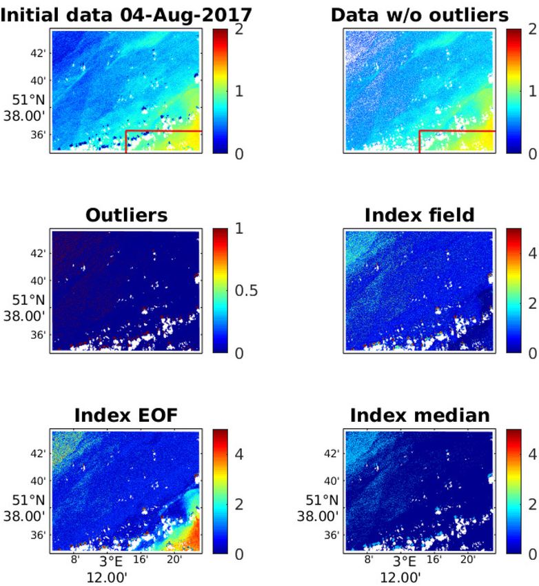
A. Alvera-Azcárate et al. Remote Sensing of Environment 253 (2021) 112229
(i.e. Zhu, Z. and Wang, S. and Woodcock, C.E., 2015; Frantz et al., 2018; 2. Data used
Qiu et al., 2019) that work with satellites without thermal band, like
Sentinel-2. Another approach is using neural networks to detect cloud 2.1. Satellite data
shadows (i.e. Hughes and Hayes, 2014), which can provide information
on clouds shadows independently on the spectral bands present in a Sentinel-2 with the MSI payload (S2/MSI) was launched by European
satellite. Most of the mentioned works have been applied to land sat Space Agency (ESA) in June 2015. The S2/MSI sensor has 13 bands in
ellite scenes, and very few deal with cloud shadow detection over the the visible ranges with spatial resolution ranging from 10 to 60 m, and a
ocean. Detection of cloud shadows over water is challenging because of 20 m resolution in the red to near-infrared (NIR) bands. The S2/MSI
its dark colour, which results in very similar spectral characteristics to level 1C (L1C) products were obtained from the Copernicus Open Access
those of cloud shadows. The complexity of cloud top altitude variations Hub, as orthorectified 100 km × 100 km2 tiles (ortho-images in UTM/
makes it very difficult to know at which distance from the cloud the WGS84 projection). The L1C products provide per-pixel Top Of Atmo
shadows can be actually located. Moreover, the large spatial variability sphere (TOA) reflectances with the parameters to transform them into
of coastal turbid waters results in a very complex field with correct low radiances.
SPM values and shadows intermingled in a single image. Temporal The S2/MSI L1C tiles were processed with ACOLITE (v20180925,
variability can be also very high, specially in the presence of strong Dark Spectrum Fitting) to generate level 2 (L2) remote sensing reflec
currents, tidal-induced resuspension of bottom sediments or estuary tance ρw(λ) products. ACOLITE performs the atmospheric correction
discharges. This makes also difficult the exploitation of temporal co using the “dark spectrum fitting” approach for coastal and inland water
herency in the time series, specially for data from satellites like Sentinel- applications (Vanhellemont and Ruddick, 2018). Non-water pixels (i.e.
2, which have a revisit time of 5 days. land, cloud contamination) are flagged using the shortwave infrared
The objective of this work is to derive a shadow detection approach (SWIR) band following the criteria: ρw(1610) > 0.0215. An additional
for high resolution sensors like Sentinel-2 over oceanic waters, by per cirrus cloud detection is performed based on the 1375 nm spectral band
forming a series of tests on specific geophysical variables (SPM and CHL using ρw(1375) > 0.005. SPM concentration (gm− 3) products were
in this case) to ensure that the approach can be applied to any sensor, generated using the algorithm of Nechad et al. (2010):
independently of the spectral bands available. The tests include a de
Aρ ρw
parture from an Empirical Orthogonal Function (EOF) basis obtained by SPM = + Bρ (1)
1 − (ρw /Cρ )
DINEOF (Data Interpolating Empirical Orthogonal Functions, Beckers
and Rixen (2003); Alvera-Azcárate et al. (2005)), as well as a threshold where Aρ (gm− 3), Bρ (gm− 3) and Cρ (unitless) are constant values which
test and a test on the proximity to identified clouds. We have also mainly depend on the water inherent optical properties and were set to
investigated the effect of adding a ray tracing test to reinforce the 610.94, 0 and 0.2324 respectively for the 665 nm spectral band. For the
penalisation of zones most probably affected by cloud shadows. A satellite data application Bρ is set to zero because the satellite sensor and
description of the Sentinel-2 data used and the domain of study is made processing will probably have different measurement errors from the
in Section 2. The proposed methodology to detect shadows is then calibration data.
described in Section 3. The results and their validation are presented in The CHL product is derived from a combination of two compatible
Sections 4 and 5 respectively and the conclusions and future outlook are algorithms: the O’Reilly blue-green band ratio OC3 algorithm (O’Reilly
presented in Section 6. et al., 2000) and the red/Near-Infrared band ratio Gons algorithm (Gons
et al., 2002, 2005). The OC3 algorithm was designed for open ocean
Fig. 1. Domain of study, containing the Belgian Coastal Zone and part of the southern North Sea. Isobaths for 20 m depth are shown, as well as the location of the
windmill parks (in blue). The different squares show the position of the subdomains given as examples in the Results Section 4.
2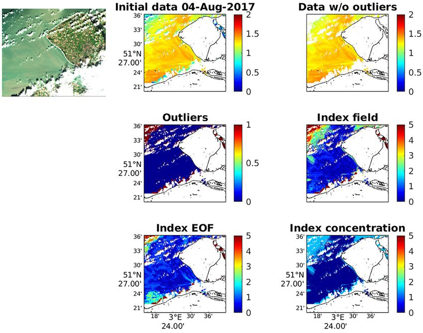
A. Alvera-Azcárate et al. Remote Sensing of Environment 253 (2021) 112229
waters and the Gons algorithm for eutrophic and turbid coastal waters. 2.3. Study areas
Pixel-based dynamic switching between these algorithms is performed
based on best suited algorithm/water type combination as described in The cloud shadow detection is first applied to the Belgian Coastal
Van der Zande et al. (2019). Zone (Fig. 1) in the southern North Sea. This zone comprises high SPM
near the coast and a strong offshore decreasing gradient. The high SPM
concentration near the coast is due to the discharge of the Scheldt, Rhine
2.2. Manual cloud shadow identification
and Meuse rivers in the Scheldt-Rhine estuary (located in the eastern
part of the domain), and therefore the temporal variability of SPM
Cloud shadows were manually identified for validation purposes by a
concentration is largely dependent on river discharge. The North Sea
human operator using the RGB images for the S2/MSI scenes for 29 April
shelf is very shallow, with an average depth of 30 m in the large domain
2017 and 4 August 2017 on the Belgian Coastal Zone. The RGB images
shown in Fig. 1, and an average depth of 15 m in the domain of study.
were imported in GIMP (v2.10.2) and cloud shadows were selected
Tidal currents therefore also play an important role in determining SPM
using the ‘Bucket Fill’ tool enabling an automated selection of pixels
concentration and dynamics, through deposition and resuspension.
based on the selected foreground colour. The number of filled pixels
A second domain of study is the Venice area. This region presents in
depends on the Fill threshold. The fill starts at the point selected by the
general lower values of SPM although river discharge results in high
operator and spreads outward until the colour value becomes “too
SPM values intermitently. The amount of clouds is lower than in the
different” from the selected pixel. The optimal threshold was selected
Belgian Coastal Zone, and shadows are less prominent. This region will
through trial and error to obtain the best coverage of the considered
be used therefore to test whether our shadow detection approach can
cloud shadow. While this approach worked well in turbid waters and
deal with these characteristics.
opaque clouds casting clearly defined shadows on the scattering waters,
it was more difficult in clear absorbing waters where the colour differ
3. Detection of shadows: method description
ence caused by clouds was minimal compared to clear water pixels. In
these conditions it was difficult to manually identify the borders of the
The shadows in high spatial resolution datasets like S2/MSI can have
cloud shadow. Similarly, shadows cast by thin clouds are blurry and
very different sizes, and represent therefore a multi-scale problem.
difficult to clearly define. The manual identification of the cloud
Shadows can have all forms and sizes: from the large cumulus clouds
shadows took 10 to 15 h per image highlighting the need for an auto
casting shadows that can be several kilometers wide, to the thin and
mated detection approach.
Fig. 2. Shadow detection example on 4 August 2017 (RGB view in the top left insert). From bottom to top: bottom left and right panels show the result of OEOF and
Oconc respectively. The middle right panel show the Ofinal index, from which a threshold of 2 is applied to determine which pixels are shadows. The final shadow/non-
shadow mask is shown in the middle left panel. Top left panel shows the initial SPM data, with very low values corresponding to cloud shadows. Top right panel
shows the final image after shadows have been removed.
3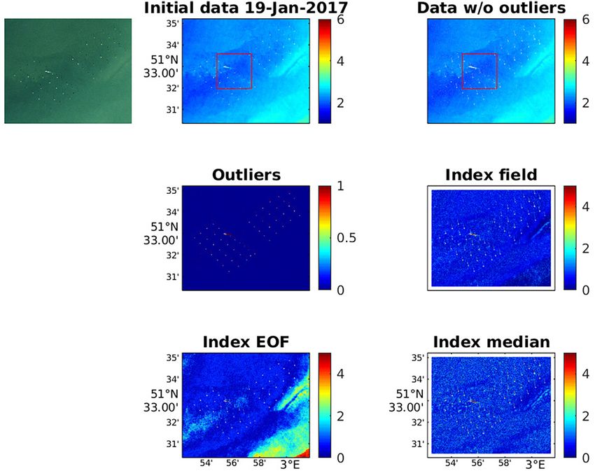
A. Alvera-Azcárate et al. Remote Sensing of Environment 253 (2021) 112229
relatively small windmill masts, which are less than 100 m long. • Proximity index, Oprox: Typically, pixels surrounding clouds are more
In order to detect shadows at different spatial scales, a set of different likely to exhibit a shadow in their vicinity. This test gives a value of 1
tests are performed on the data. These tests build on the outliers to pixels immediately surrounding an already missing value (cloud,
detection approach described in Alvera-Azcárate et al. (2012, 2015), in land, bad data masked for quality reasons) and zero otherwise. This
which outliers were detected in medium spatial resolution data (sea test can be applied iteratively to reach further away from the cloud or
surface temperature from AVHRR and turbidity from SEVIRI, respec land edges.
tively). In this approach, individual pixels with a behavior distinct from • Concentration test, Oconc: The presence of shadows in ocean colour
their neighboring pixels were targeted, but given the spatial extension of variables is always associated to low values of the variable being
cloud shadows, these cannot be detected using directly the approach in analysed relative to the surrounding clear water pixels. However, as
Alvera-Azcárate et al. (2012, 2015). The detection of shadows in high already mentioned, these are still within the range of plausible
resolution data needs the addition of some tests adapted to the problem. values, and cannot be detected as outliers by applying a fixed
The tests are described as follows: threshold. To overcome this, a varying threshold is instead applied,
which depends on the amount of missing data in each individual
• EOF index, OEOF: A first test determines the departure of each pixel image and the quantile distribution of the values of the variable used
from an EOF basis calculated from the data being analysed. This EOF (SPM concentration or CHL in this case). The higher the percentage
basis is calculated using DINEOF (Beckers and Rixen, 2003; Alvera- of missing data (%MD) of a given image, the higher the quantile
Azcárate et al., 2005) to overcome the problem of missing data. The below which data are considered suspect. The concentration test is
EOF basis is truncated by retaining only the modes that minimise the only applied when %MD > 20%:
error of the reconstruction. Transient and localized features like
data > Q%MD/100 →Oconc = 0; (else Oconc = 1) (2)
shadows are therefore not part of the EOF basis and can be identified
by its departure from it. The mean absolute difference between an The rationale behind this setting is that, the higher the percentage of
original pixel and the estimation obtained by the truncated EOF basis missing data on a given image (and therefore of clouds), the more
is calculated. This test provides a departure index with values probable that a given clear pixel is a shadow. As an example, if a given
starting from zero (no difference between a pixel and the EOF basis at image has 10% of missing data, and the 10th quantile for all the values of
that point) and with an unbounded positive value for pixels differing that same image is 0.3, then all pixels with an SPM value smaller than
from the EOF basis. 0.3 gm− 3 will be given a Oconc = 1. If that same image has 15% of missing
data, and the 15th quantile is 0.47, then all pixels with an SPM value
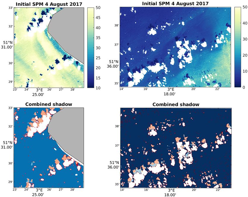
Fig. 3. Shadow detection example on 4 August 2017
in an open domain containing the northwest corner of
Fig. 2 (shown by the red line). From bottom to top:
bottom left and right panels show the result of OEOF
and Omedian respectively. The middle right panel show
the Ofinal index, from which a threshold of 2 is applied
to determine which pixels are shadows. The final
shadow/non-shadow mask is shown in the middle left
panel. Top left panel shows the initial SPM data, with
very low values corresponding to cloud shadows. Top
right panel shows the final image after shadows have
been removed. (For interpretation of the references to
colour in this figure legend, the reader is referred to
the web version of this article.)
4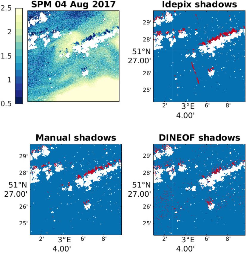
A. Alvera-Azcárate et al. Remote Sensing of Environment 253 (2021) 112229
Fig. 4. Shadow detection example on 1 January 2017 in the C-Power offshore windmill park (RGB view in the top left insert). From bottom to top: bottom left and
right panels show the result of OEOF and Omedian respectively. The middle right panel show the Ofinal index, from which a threshold of 2 is applied to determine which
pixels are shadows. The final shadow/non-shadow mask is shown in the middle left panel. Top left panel shows the initial SPM data, with very low values corre
sponding to windmill shadows, and very large values associated with a ship wake. Top right panel shows the final image after shadows and wake have been removed.
Red squares in the top row indicate the domain shown in Fig. 5. (For interpretation of the references to colour in this figure legend, the reader is referred to the web
version of this article.)
3
smaller than 0.47 gm− will be given a Oconc = 1. An index Ofinal is finally calculated as the weighted sum of the three
mentioned tests:
• Median test, Omedian: the difference between a given pixel and a local
Ofinal = W1 OEOF + W2 Oprox + W3 Oconc (3)
median calculated over a 30 × 30 box, normalized by the mean
absolute deviation calculated over the same domain, is calculated.
with W1, W2 and W3 the weights applied to each test. These weights can
Departures from this median are penalised. This test is only applied if
change depending on the data and the objectives, and the specific values
the percentage of missing data is lower than 20%, as the computa
used in this work will be presented in Section 4. In the case of having less
tional cost is high and this test is most efficient in detecting very
than 20% of missing data in a given image, the concentration test Oconc is
small shadows on clear days (like windmill mast shadows). The size
substituted by the median test Omedian:
of the box has been chosen to concentrate in small-scale features.
Fig. 5. Detail of the red insert of Fig. 4. Left panel shows initial SPM and right panel shows SPM after removal of shadows and other suspect data, as the ship wake.
(For interpretation of the references to colour in this figure legend, the reader is referred to the web version of this article.)
5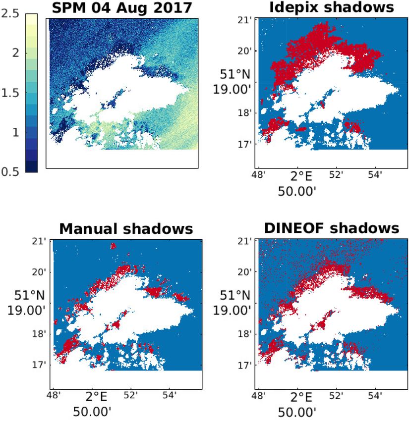
A. Alvera-Azcárate et al. Remote Sensing of Environment 253 (2021) 112229
Ofinal = W1 OEOF + W2 Oprox + W4 Omedian (4) described in Section 2. Given the very large size of S2/MSI data, the
DINEOF reconstruction was applied to subsets of data, covering each 1/
All weights can be adjusted to the characteristics of the variable and
4th of the domain shown in Fig. 1. Examples of results in some of these
region of interest.
subsets are shown here.
An additional test can be added, in line with other existing cloud
The specific weight of each subtest described in Section 3 was
shadow detection methods, to estimate the probable location of the
determined first by establishing which tests had a larger impact in the
shadow given the position of a cloud. A ray tracing approach has been
detection of shadows. The truncated EOF basis used to calculate OEOF
adopted, and can be described as follows:
consisted of 3 EOFs (determined by cross-validation by DINEOF). For
images with more than 20% of missing data, Oconc and OEOF played the
• Ray tracing test, Oray: For every pixel of the scene, we compute the
largest roles, and for images with less than 20% of missing data, it was
position of the sun in the sky using the Julia package AstroLib. We
Omedian that best helped detecting shadows. Given this, and after trying
assume that the altitude of the clouds is known and constant. The
several combinations, the following weights were used:
cloud layer is represented by a binary mask (0 clear sky and 1
covered sky). We computed the ray connecting a given pixel and the
• More than 20% of missing data: W1 = 0.8; W2 = 0.2; W3 = 0.2
sun and then determined where this ray would intersect the cloud
• Less than 20% of missing data: W1 = 0.2; W2 = 0.2; W4 = 0.8
layer. If the nearest point to this intersection is a cloud, then the pixel
has a shadow index of 1. Otherwise it has an index of 0.
The level above which a pixel is classified as shadow was fixed at 2
after some trials. Therefore, it was decided that pixels providing a value
We have used the ray tracing test by establishing a top of the cloud
of 1 in the Oconc test, when more than 20% of missing data are present,
height of 1.5 km, which is of course not always the case. However, the
are automatically classified as shadow. The OEOF and Oprox tests help in
ray tracing test is used only to provide a probable area of suspicious
finding some other pixels that are not correctly classified as shadow by
pixels, and it is most useful when thin and scattered clouds are present.
the Oconc test alone. In this first domain, the ray tracing test was not used
The combination of the four tests and their weights determines if a pixel
since it didn’t have a measurable impact in the final shadow detection.
is shadowed or not. If the ray tracing test is applied, it is added to the
An example of shadow detection for 4 August 2017 is shown in Fig. 2,
previous one: Ofinal = Ofinal + Oray.
covering domain 1 as shown in Fig. 1. The amount of missing data on
this day is 25%. The cloud shadows located along the southern coast are
4. Results
correctly detected, as well as the scattered shadows in the middle of the
domain. There is one zone in the northwest corner of the domain that
4.1. Detection of cloud shadows in the Belgian Coastal Zone
presents a large amount of false positives (i.e. pixels classified as
shadows that are valid SPM data) since both Oconc and OEOF classify these
The shadow detection approach was applied to the 2017 S2/MSI data
Fig. 6. Shadow detection example on 29 August 2019 in
domain 4 (see RGB view top left). From bottom to top: bot
tom left and right panels show the result of OEOF and Oconc
respectively. The middle right panel show the Oray index,
with 1 to pixels affected by a cloud. The final shadow/non-
shadow mask is shown in the middle left panel. Top left
panel shows the initial SPM data, with very low values cor
responding to cloud shadows. Top right panel shows the final
image after shadows have been removed.
6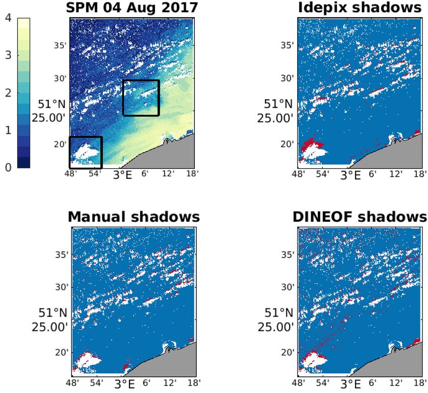
A. Alvera-Azcárate et al. Remote Sensing of Environment 253 (2021) 112229
Fig. 7. Shadow detection example on 6 October 2019 in the Venice area (see insert map bottom left and RGB view top left). From bottom to top: bottom left and right
panels show the result of OEOF and Oconc respectively. The middle right panel show the Oray index, with 1 to pixels affected by a cloud. The final shadow/non-shadow
mask is shown in the middle left panel. Top left panel shows the initial SPM data, with very low values corresponding to cloud shadows. Top right panel shows the
final image after shadows have been removed.
pixels as suspect. This zone is characterized by low values of SPM, which the Omedian test. The shadows of the windmills are correctly detected by
suggests that the accuracy of the shadow detection can be improved if our approach. The wake of a ship crossing the wind farm results in
the detection of shadows for that zone would be made separately, for erroneous high SPM concentration values, and these pixels are also
example by determining a domain of open waters, with low values of detected as shadows. Since our approach can also detect features that
SPM. are anomalous with respect to their surroundings, the detection of such
To test this idea, an open waters domain containing the northwestern erroneous data is also possible.
corner of Fig. 2 is used to test if the detection of shadows is improved in A detail of this figure is shown in Fig. 5, in which the detection of the
that corner. Fig. 3 shows the shadow detection in domain 2 (Fig. 1), with windmill masts shadows is more clearly seen. This figure also shows that
the same tests as in Fig. 2 except for Oconc test which is replaced by the the turbid wakes created by the current flowing through the windmill
Omedian, as the amount of missing data in domain 2 for 4 August is of 4%. masts (e.g. Vanhellemont and Ruddick, 2014), in a west-southwest di
It can be seen that the cloud shadows are now more accurately detected rection from the masts, are (correctly) not detected as anomalous,
in the overlapping corner. The approach presented is therefore able to contrary to the ship wake.
work in domains with lower SPM concentration values, where the
shadows are not so clearly visible. A careful compositing to reunite all
subscenes after shadow detection is of course needed. 4.3. Shadow detection in chlorophyll data in the Belgian Coastal Zone
In order to test the accuracy of the shadow detection in a different
4.2. Detection of windmill shadows setting, a test has been made using CHL data in 2019 in domain 4 of
Fig. 1. The dataset used consists of 77 images spanning from 9 January
The presence of shadows from other sources than clouds is also 2019 to 2 December 2019 (images that have more than 96% of missing
visible in high spatial resolution satellite data. Offshore windmill farms data have been removed). After realising some tests with different
are being developed quickly in many places around the globe, including weights for each of the subtests, it was decided that the same combi
the North Sea. Our domain of study contain three farms (either finished nation of tests (i.e. W1 = 0.8; W2 = 0.2; W3 = 0.2 for more than 20% of
or under construction): Norther, C-Power and Northwind. The shadow missing data) led to satisfying results. The ray tracing test was also used
detection has been applied to a domain containing the C-Power wind in this example, since we observed the presence of thin and scattered
farm (domain 3 in Fig. 1), and the results on a very clear day (19 January clouds. The threshold to decide whether a pixel is a cloud shadow or not
2017, with 0% of missing data) are shown in Fig. 4. In this case, as the was set to 1.5 (instead of 2 with SPM). While we have kept the same
amount of missing data is smaller than 20%, the Oconc test is replaced by values as the previous examples, these need to be adjusted to the
7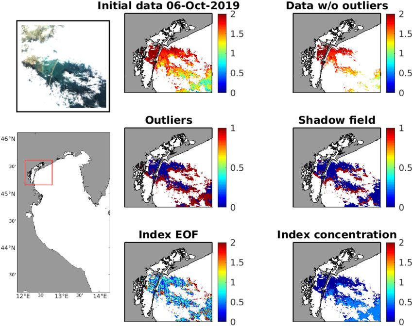
A. Alvera-Azcárate et al. Remote Sensing of Environment 253 (2021) 112229
Two more examples are given for small scattered clouds, on 4 August
2017 (Fig. 9). First on the eastern part of the domain (domain 6, shown
in the left column of Fig. 9). On this part of the domain, 85.20% of the
pixels detected manually as being shadows have been detected by our
approach. A 4.10% of the open-sea data (i.e. no clouds nor shadows) are
classified as shadows by our approach but not manually, but again, this
percentage includes false positives and pixels not detected manually but
that are shadows. The second example is given for domain 2, and it is
shown in the right column of Fig. 9. On this part of the domain, 75.22%
of the pixels detected manually as being shadows have been detected by
our approach. A 1.21% of the open-sea data (i.e. no clouds nor shadows)
are classified as shadows by our approach but not manually, a per
centage that includes false positives and pixels not detected manually
but that are shadows. In this specific frame, close inspection of the
scattered pixels detected with our approach shows they are mostly
whitecaps in the initial data, and have been identified as suspect data.
5.2. Comparison with Idepix
While the comparison with manually detected shadows provides a
very good frame to objectively assess the accuracy of the results, it is
interesting to assess how our approach compares with other existing
automated approaches for detection of cloud shadows. For the example
Fig. 8. Cloud shadow detection on 29 April 2017. Top panel shows SPM values, on 4 August 2017 we can therefore assess the accuracy of our method
with low values (dark blue) due to shadows, and clouds in white. Bottom panel and the accuracy obtained with Idepix, a S2/MSI cloud shadow pro
shows pixels detected as cloud both manually and by the present methodology cessor developed for the SNAP (Sentinel Application Platform) software
(pink), pixels detected manually but not by our method (light blue) and pixels (Lebreton et al., 2016). Idepix combines the cloud mask with sun ge
detected by our method but not manually (red). (For interpretation of the ometry to search regions of maximum probability for shadow pixels. As
references to colour in this figure legend, the reader is referred to the web no cloud height is available for S2/MSI data, a maximum cloud height is
version of this article.) predetermined as a function of latitude. Within the projected region of
potential cloud shadow, the cloud mask is shifted towards the surface
variable and domain of study. An example on 29 August 2019 is pre reflectance minimum along the illumination path. These pixels are
sented in Fig. 6, with all the subtests as in previous examples. Shadows flagged as IDEPIX_CLOUD_SHADOW. Additionally, pixels within the
are generally well detected, and the addition of ray tracing is useful for potential shadow area are clustered based on surface reflectances and
some shadows near the southwest corner. the darkest cluster is flagged as IDEPIX_CLUSTERED_CLOUD_SHADOW.
Both flags were combined to a single cloud shadow flag in this study.
4.4. Shadow detection in SPM data on the Venice area The whole domain for 4 August 2017 is shown in Fig. 10, together
with the shadows detected manually, with Idepix and with our
The shadow detection approach has been also tested in a different approach. It can be seen that our approach shows more scattered pixels
region. S2/MSI SPM data in the Venice area from 2019 were chosen, as that have been detected as shadows but do not appear in the manual
this region presents very different values in SPM than the Belgian mask (especially in the southwest corner). On the other hand, Idepix
Coastal Zone. The weights were again maintained as in the 2 previous seems to have overestimated the shadow for the large cloud situated in
tests, adding the ray tracing test as well. The threshold to classify a pixel the southwest, and presents also some scattered clouds near the coast
as shadow or not was set to 2. An example on 6 October 2019 is pre not detected manually. In order to assess the accuracy of each method,
sented in Fig. 7, again showing that most shadows are correctly we will zoom in these two places, marked with a square in Fig. 10.
identified. Fig. 11 shows the first zoomed image. Compared with the manual
shadow mask, our approach detects 82.30% of the shadows, with 9.70%
5. Validation of false positives, which appear to be scattered shadows north of the
cloud associated with low concentration SPM values. Idepix on the other
5.1. Cloud shadow detection in the Belgian Coastal Zone SPM dataset hand, has a too large cloud shadow, and compared with the manual
mask it detects 65% of them. In terms of false positives in Idepix,
In order to assess the accuracy of our approach, we have selected 2 because of the large shadow, this value goes up to 18%. The second
scenes in which cloud shadows have been detected manually: 29 April zoom is presented in Fig. 12. Here our approach detects too few
2017 and 4 August 2017 in the Belgian Coastal Zone. As described in shadows, summing up to 50% of the manual shadows and 1.9% of false
Section 2.2, shadows were detected manually along the domain of study positives. Idepix detects 60% of the manual shadows, with 1.6% of false
by individually selecting all pixels identified as shadow. While this is a positives. We can see an artifact in the Idepix detected shadows in the
long and tedious work to realise, it also provides a very strict validation form of a line, and again some scattered shadows for our approach.
baseline to compare our shadow detection approach with. The percentage of shadows detected in the second zoom is quite low
An example is shown in Fig. 8 for 29 April 2017. In this case, 63% of for our approach, though Idepix also underperformed with respect to the
the pixels detected manually as being shadows have been detected by results in the first zoom. This scene appeared as specially challenging for
our approach. The percentage of no-cloud pixels classified as shadows by both approaches. Close inspection of this scene reveals that our
our approach but not manually is 3%, and while these can be considered approach failed to detect thin shadows caused by the clouds edges. A
false positives, close inspection of the image shows that there are also way to improve on this would therefore be to increment the shadows by
pixels at the edges of clouds that might have been overlooked in the two or three pixels around the detected shadows. The number of false
manual detection. positives would however also increase.
8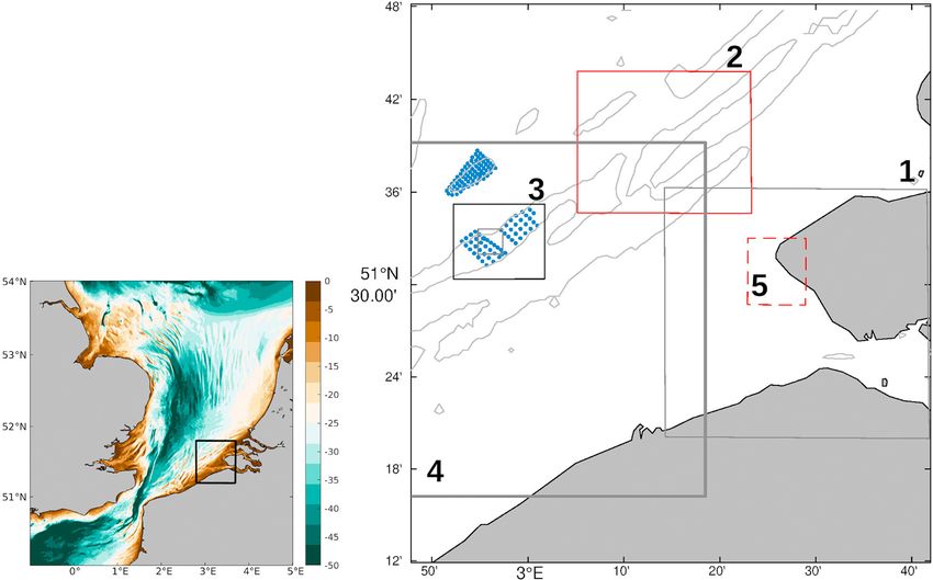
A. Alvera-Azcárate et al.                                                                                          Remote Sensing of Environment 253 (2021) 112229

Fig. 9. Cloud shadow detection on two subdomains on 4 August 2017. Top left panel (east domain) shows SPM values, with low values (dark blue) due to shadows,
and clouds in white. Bottom left panel shows pixels detected in the east domain as cloud both manually and by the present methodology (pink), pixels detected
manually but not by our method (light blue) and pixels detected by our method but not manually (red, mostly at some cloud edges). Top right panel (northwest
domain) shows SPM values, with low values (dark blue) due to shadows, and clouds in white. Bottom left panel shows pixels detected in the northwest domain as
cloud both manually and by the present methodology (pink), pixels detected manually but not by our method (light blue) and pixels detected by our method but not
manually (red, mostly at some cloud edges). (For interpretation of the references to colour in this figure legend, the reader is referred to the web version of
this article.)

                                                                               9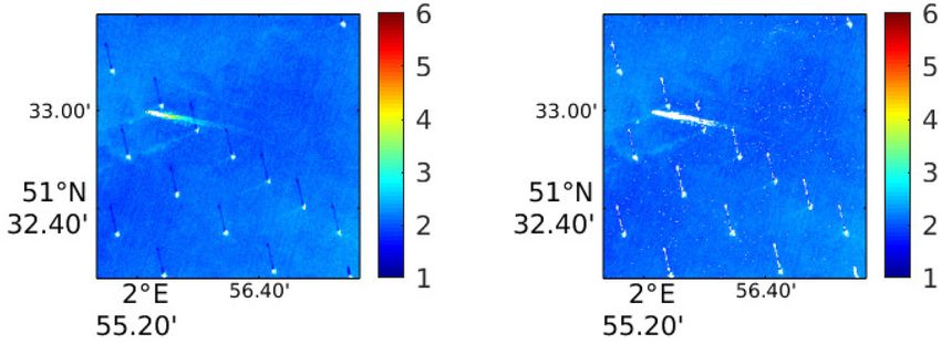
A. Alvera-Azcárate et al.                                                                                                  Remote Sensing of Environment 253 (2021) 112229

Fig. 10. Cloud shadow detection on domain 4, for 4 August 2017. Top left panel shows SPM values, with low values (dark blue) due to shadows, and clouds in white.
Bottom left panel shows pixels detected as shadow manually (in red). Top right panel shows the shadows detected by Idepix, and the bottom right panel shows the
shadows detected by the present method. (For interpretation of the references to colour in this figure legend, the reader is referred to the web version of this article.)

                                                                                   10
A. Alvera-Azcárate et al. Remote Sensing of Environment 253 (2021) 112229
Fig. 11. Cloud shadow detection on the first zoom of
domain 4, for 4 August 2017. Top left panel shows
SPM values, with low values (dark blue) due to
shadows, and clouds in white. Bottom left panel
shows pixels detected as cloud manually (in red). Top
right panel shows the shadows detected by Idepix,
and the bottom right panel shows the shadows
detected by the present method. (For interpretation
of the references to colour in this figure legend, the
reader is referred to the web version of this article.)
5.3. Chlorophyll BCZ dataset validation 6. Discussion and conclusions
For the validation of the CHL shadow detection in the Belgian Coastal A method to detect shadows in high spatial resolution ocean satellite
Zone we have the results of our approach and from Idepix. Because none data has been described. The method detects shadows of various sizes,
of these two can be considered the truth, it is more a comparison exercise from large clouds down to the masts of offshore windmills. Large cloud
than a validation, although visual inspection can already give a good shadows can affect the quality of the images and hence the analysis
estimate about the shadow detection accuracy of each method. First, the derived from them, but also at the mast-scale size, undetected shadows
results of the subtests are presented in Fig. 13. It can be seen that both can have a net influence in studies aiming at assessing the impact of
approaches identify most of the shadow pixels present in the left panel. offshore windmill parks in the total quantity of suspended matter.
The present method still has some scattered pixels detected as shadows, The methodology proposed is based on a series of tests applied
but on the other hand it also detects correctly that some pixels in the low directly to the physical variables derived from the satellite measured
left corner, close to the coast, are probably not shadow. Idepix classifies radiances. It does not depend therefore in the characteristics of the
all these as shadow. If we were to consider Idepix as the truth, our satellite sensor (wavebands measured) and can be applied to any sat
approach detects 70.5% of Idepix shadows, and Idepix classifies as no ellite. The data used in this work was suspended particulate matter
shadow 12.5% of pixels classified as shadow in our approach. (SPM) and chlorophyll (CHL) measured by Sentinel-2, and two domains
(Belgian Coastal Zone and Venice) and periods (2017 and 2019) were
5.4. SPM Venice dataset validation analysed. The tests include a departure from a truncated EOF basis
calculated from a time series of images (large departures are penalised),
For the SPM dataset in Venice, a comparison with Idepix is also done. a threshold test (low values are penalised), a proximity test (pixels
The results are presented in Fig. 14 for Idepix and our approach. This adjacent to missing data are penalised), and a median test in images with
case, with a large cloud cover over most of the scene, seemed to be more low percentage of missing data (departures from local median are
difficut for Idepix, which ended up classifying large zones as shadow, penalised). A ray tracing test can also be used, which calculates the path
while clearly these are not shadowed in the left panel. Idepix took more between each pixel and the Sun to determine if there is a cloud pro
than 20 h of computation for this single scene. Our approach looks closer jecting a shadow. This test has proved to be useful in the presence of thin
to what the actual shadows are. Comparing again the percentage of and scattered clouds, and therefore we recommend its use along the rest
pixels detected as shadows in each technique, there are 54% of Idepix of the tests. These various tests can be weighed differently depending on
shadows that have been classified as shadows by our approach, and 29% the dataset used, and the threshold above which data are discarded can
of shadows in our approach that have not been classified as shadows in also be adjusted.
Idepix. The results were compared to manually selected cloud shadows, and
11A. Alvera-Azcárate et al. Remote Sensing of Environment 253 (2021) 112229
Fig. 12. Cloud shadow detection on the second zoom
of domain 4, for 4 August 2017. Top left panel shows
SPM values, with low values (dark blue) due to
shadows, and clouds in white. Bottom left panel
shows pixels detected as shadow manually (in red).
Top right panel shows the shadows detected by Ide
pix, and the bottom right panel shows the shadows
detected by the present method. (For interpretation
of the references to colour in this figure legend, the
reader is referred to the web version of this article.)
Fig. 13. Cloud shadow detection on CHL data on 29 August 2019, in the domain indicated by a square in Fig. 6. Left panel: initial CHL data. Center panel: pixels
identified by Idepix as shadows (red). Right panel: pixels identified by Idepix as sadows (red). (For interpretation of the references to colour in this figure legend, the
reader is referred to the web version of this article.)
Fig. 14. Cloud shadow detection on CHL data on 6 October 2019. Left panel: initial CHL data. Center panel: pixels identified by Idepix as sadows (red). Right panel:
pixels identified by Idepix as sadows (red). (For interpretation of the references to colour in this figure legend, the reader is referred to the web version of this article.)
12A. Alvera-Azcárate et al. Remote Sensing of Environment 253 (2021) 112229
overall a good accuracy is achieved in detecting shadows. The presence Beckers, J.-M., Rixen, M., 2003. EOF calculations and data filling from incomplete
oceanographic data sets. J. Atmos. Ocean. Technol. 20 (12), 1839–1856.
of false positives were due mainly to scattered pixels classified as
Braaten, J., Cohen, W., Yang, Z., 2015. Automated cloud and cloud shadow identification
shadow, and are probably low values penalised by the concentration in Landsat MSS imagery for temperate ecosystems. Remote Sens. Environ. 169,
test. Other sources of false positives were anomalous data present in the 128–138.
image but not due to the presence of clouds. The proposed method, as it Frantz, D., Haß, E., Uhl, A., Stoffels, J., Hill, J., 2018. Improvement of the Fmask
algorithm for Sentinel-2 images: separating clouds from bright surfaces based on
penalises anomalous data independently of their absolute value, also parallax effects. Remote Sens. Environ. 215, 471–481.
detects wrong high SPM values associated with the wake of a ship, and Gons, H.J., Rijkeboer, M., Ruddick, K.G., 2002. A chlorophyll-retrieval algorithm for
whitecaps. These features are penalised by the EOF test. satellite imagery (medium resolution imaging spectrometer) of inland and coastal
waters. J. Plankton Res. 24 (9), 947–951.
A comparison with another shadow detection technique, Idepix, has Gons, H.J., Rijkeboer, M., Ruddick, K.G., 2005. Effect of a waveband shift on chlorophyll
been also performed. Depending on the frame, either Idepix or our retrieval from meris imagery of inland and coastal waters. J. Plankton Res. 27 (1),
approach performed better, compared to the manually detected pixels. 125–127.
Goodwin, N., Collett, L., Denham, R., Flood, N., Tindall, D., 2013. Cloud and cloud
Idepix seemed to overclassify possible shadow pixels, flagging large shadow screening across Queensland, Australia: an automated method for Landsat
areas which are visibly not shadows. Our approach presents scattered TM/ETM+ time series. Remote Sens. Environ. 134, 50–65.
pixels, not associated with a cloud, classified as shadows. Detecting too Huang, C., Thomas, N., Goward, S., Masek, J., Zhu, Z., Townshend, J., Vogelmann, J.,
2010. Automated masking of cloud and cloud shadow for forest change analysis
large shadows, as in Idepix, results in large areas being flagged out, using landsat images. Int. J. Remote Sens. 31 (20), 5449–5464.
which makes subsequent uses of the data more difficult. Scattered pixels Hughes, M., Hayes, D., 2014. Automated detection of cloud and cloud shadow in single-
on the other hand may have a smaller impact on the potential use of the date landsat imagery using neural networks and spatial post-processing. Remote
Sens. 6 (6), 4907–4926.
data afterwards, as these scattered points are easier to interpolate, and
Lebreton, C., Stelzer, K., Brockmann, C., Bertels, L., Pringle, N., Paperin, M., Danne, O.,
do not obscure totaly large zones of valid data. In our tests we have Knaeps, E., Ruddick, K., 2016. Cloud and Cloud Shadow Masking of High and
observed a tendency for Idepix to overestimate cloud shadows, and an Medium Resolution Optical Sensors-an Algorithm Inter-Comparison Example for
accuracy of 60–65%. Landsat 8, vol. SP-740 (URL https://www.scopus.com/inward/record.uri?eid=2-
s2.0-84988452215 partnerID=40 md5=3c1befe362880129108734bd9e04cbab).
In our proposed method, all the tests and the final detection are Luo, Y., Trishchenko, A., Khlopenkov, K., 2008. Developing clear-sky, cloud and cloud
based on a series of thresholds that can be adapted to provide more or shadow mask for producing clear-sky composites at 250-meter spatial resolution for
less strict shadow detection. Stronger thresholds will provide a larger the seven MODIS land bands over Canada and North America. Remote Sens. Environ.
112, 4167–4185.
detection accuracy, but more false positives will be also present in the Nechad, B., Ruddick, K., Park, Y., 2010. Calibration and validation of a generic
final dataset. The user can assess the thresholds best suited to their multisensor algorithm for mapping of total suspended matter in turbid waters.
application and domain of study. Remote Sens. Environ. 114 (4), 854–866.
O’Reilly, J.E., Maritorena, S., O’Brien, M.C., Siegel, D.A., Toole, D., Menzies, D.,
Smith, R.C., Mueller, J.L., Mitchell, B.G., Chavez, F.P., Strutton, P., Cota, G.F.,
Declaration of Competing Interest Hooker, S.B., McClain, C.R., Carder, K.L., Müller-Karger, F., Harding, L.,
Magnuson, A., Phinney, D., Moore, G.F., Aiken, J., Arrigo, K.R., Letelier, R.,
Culver, M., 2000. SeaWiFS Postlaunch Calibration and Validation Analyses, Part 3.
None. Tech. rep., NASA Technical Memo (49 pages).
Qiu, S., Zhu, Z., He, B., 2019. Fmask 4.0: improved cloud and cloud shadow detection in
Acknowledgments Landsats 4–8 and Sentinel-2 imagery. Remote Sens. Environ. 231.
Sun, L., Liu, X., Yang, Y., Chen, T., Wang, Q., Zhou, X., 2018. A cloud shadow detection
method combined with cloud height iteration and spectral analysis for Landsat 8 OLI
This research was performed with funding from the Belgian Science data. ISPRS J. Photogramm. Remote Sens. 138, 193–207.
Policy Office (BELSPO) STEREO III programme in the framework of the Van der Zande, D., Eleveld, M., Lavigne, H., Gohin, F., Pardo, S., Tilstone, G., Blauw, A.,
MULTI-SYNC project (contract SR/00/359). Computational resources Markager, S., Enserink, L., 2019. Joint monitoring programme of the EUtrophication
of the NOrth Sea with SATellite data user case in Copernicus marine service ocean
have been provided by the Consortium des Équipements de Calcul state report. J. Oper. Oceanogr. 12 (3), 1–123.
Intensif (CÉCI), funded by the Fonds de la Recherche Scientifique de Vanhellemont, Q., Ruddick, K., 2014. Turbid wakes associated with offshore wind
Belgique (F.R.S.-FNRS) under Grant No. 2.5020.11 and by the Walloon turbines observed with Landsat 8. Remote Sens. Environ. 145, 105–115.
Vanhellemont, Q., Ruddick, K., 2018. Atmospheric correction of metre-scale optical
Region. The authors wish to thank the useful feedback provided by three satellite data for inland and coastal water applications. Remote Sens. Environ. 216,
anonymous reviewers. 586–597.
Zhai, H., Zhang, H., Zhang, L., Li, P., 2018. Cloud/shadow detection based on spectral
indices for multi/hyperspectral optical remote sensing imagery. ISPRS J.
References Photogramm. Remote Sens. 144, 235–253.
Zhu, Z., Woodcock, C., 2012. Object-based cloud and cloud shadow detection in Landsat
Alvera-Azcárate, A., Barth, A., Rixen, M., Beckers, J.-M., 2005. Reconstruction of imagery. Remote Sens. Environ. 118, 83–94.
incomplete oceanographic data sets using empirical orthogonal functions. Zhu, Z., Woodcock, C., 2014. Automated cloud, cloud shadow, and snow detection in
Application to the Adriatic Sea surface temperature. Ocean Model. 9, 325–346. multitemporal Landsat data: an algorithm designed specifically for monitoring land
https://doi.org/10.1016/j.ocemod.2004.08.001. cover change. Remote Sens. Environ. 152, 217–234.
Alvera-Azcárate, A., Sirjacobs, D., Barth, A., Beckers, J.-M., 2012. Outlier detection in Zhu, Z., Wang, S., Woodcock, C.E., 2015. Improvement and expansion of the Fmask
satellite data using spatial coherence. Remote Sens. Environ. 119, 84–91. algorithm: cloud, cloud shadow, and snow detection for Landsats 4-7, 8, and sentinel
Alvera-Azcárate, A., Vanhellemont, Q., Ruddick, K., Barth, A., Beckers, J.-M., 2015. 2 images. Remote Sens. Environ. 159, 269–277.
Analysis of high frequency geostationary ocean colour data using DINEOF. Estuar.
Coast. Shelf Sci. 159, 28–36.
13You can also read