Case History Hockley Fault revisited: More geophysical data and new evidence on the fault location, Houston, Texas - Squarespace
←
→
Page content transcription
If your browser does not render page correctly, please read the page content below
GEOPHYSICS, VOL. 83, NO. 3 (MAY-JUNE 2018); P. 1–10, 14 FIGS.
10.1190/GEO2017-0519.1

Case History

Hockley Fault revisited: More geophysical data and new evidence
on the fault location, Houston, Texas

Mustafa Saribudak1, Michal Ruder2, and Bob Van Nieuwenhuise3

                                  ABSTRACT                                   section. Farther north across Highway 290, the resistivity data
                                                                             and the presence of fault scarps indicate that the Hockley Fault
       Ongoing sediment deposition and related deformation in the            appears to be offset to the east, which has not been previously
    Gulf of Mexico cause faulting in coastal areas. These faults             documented. The publicly available LiDAR data and historical
    are aseismic and underlie much of the Gulf Coast area including          aerial photographs of the study area support our geophysical
    the city of Houston in Harris County, Texas. Considering that            findings. This important geohazard result impacts the mitigation
    the average movement of these faults is approximately 8 cm per           plan for the Hockley Fault because it crosses and deforms High-
    decade in Harris County, there is a great potential for structural       way 290 in the study area. The nonunique model of the gravity
    damage to highways, utility infrastructure, and buildings that           and magnetic data indicates strong correlation of a lateral
    cross these features. Using integrated geophysical data, we have         change in density and magnetic properties across the Hockley
    investigated the Hockley Fault, located in the northwest part of         Fault. The gravity data differ from the expected signature. The
    Harris County across Highway 290. Our magnetic, gravity, con-            high gravity observed on the downthrown side of the fault is
    ductivity, and resistivity data displayed a fault anomaly whose          probably caused by the compaction of unconsolidated sedi-
    location is consistent with the southern portion of the Hockley          ments on the downthrown side. There is a narrow zone of rel-
    Fault mapped by previous researchers at precisely the same               ative negative magnetic anomalies adjacent to the fault on the
    location. Gravity data indicate a significant fault signature that       downthrown side. The source of this magnetization could be due
    is coincident with the magnetic and conductivity data, with rel-         to the alteration of mineralogies by the introduction of fluids
    atively positive gravity values observed in the downthrown               into the fault zone.

                           INTRODUCTION                                         Based on a study of borehole logs and seismic reflection
                                                                             data, faults have been delineated to depths of 3660 m below the
   The coastal plain of the Gulf of Mexico is underlain by a thick           surface (Kasmarek and Strom, 2002). The activation of these faults
sequence of largely unconsolidated, lenticular deposits of clays and         on the topographic surface may have resulted from natural geologic
sands that are cut with faults (Verbeek and Clanton, 1981). These            processes such as salt movement and fluid extraction (oil and gas
faults are primarily identified as growth faults, which are prevalent        and ground water) (Sheets, 1971; Paine, 1993). Historically, these
in Harris County and throughout the coastal areas of Texas and Lou-          faults have played a significant role in oil and gas exploration, and
isiana. Growth faults are a particular type of normal fault that de-         significant hydrocarbon accumulations are attributed to the pres-
velops during ongoing sedimentation such that the strata on the              ence of growth faults (Ewing, 1983; Shelton, 1984).
hanging-wall side of the fault tend to be thicker than those on                 Since the late 1970s and early 1980s, the USGS launched an
the footwall side (Figure 1).                                                extensive fault study in the greater Houston area (Clanton and

   Manuscript received by the Editor 5 August 2017; revised manuscript received 5 January 2018; published ahead of production 11 February 2018.
   1
     Environmental Geophysics Associates, Austin, Texas, USA. E-mail: mbudak@pdq.net.
   2
    Wintermoon Geotechnologies Inc., Glendale, Colorado, USA. E-mail: meruder@wintermoon.com.
   3
    Deceased. Earth-Wave Geosciences, Houston, Texas, USA. E-mail: dvnieuwe@central.uh.edu.
     © 2018 Society of Exploration Geophysicists. All rights reserved.

                                                                         1
2                                                                  Saribudak et al.

Amsbury, 1975; Verbeek and Clanton, 1978; Verbeek, 1979; Clan-                   and mapping of these active faults is important so that developers
ton and Verbeek, 1981; O’Neill and Van Siclen, 1984), and since                  can avoid building in their vicinity. Furthermore, a thorough geo-
then, hundreds of active faults have been identified. Today, there are           logic understanding of these faults is critical to minimize and mit-
more than 350 known growth faults in the Houston area.                           igate against their geohazard impact.
   These active faults disturb the surface in the Houston-Galveston                 The objective of this work is to provide additional geophysical data
region (Clanton and Amsbury, 1975; Clanton and Verbeek, 1981).                   (magnetic, conductivity, and gravity) on the Hockley Fault and to
These include the Long Point, Hockley, Addicks, Tomball, Willow                  determine the accurate location of the fault across Highway 290. Fig-
Creek, and Eureka Faults (Saribudak, 2011a, 2011b). Evidence of                  ure 2 shows the Hockley Fault and the study area. The site map is
faulting is visible from structural damage such as fractures and/or              taken from Khan et al. (2013), and it displays airborne LiDAR data.
displacement of buildings, utility lines, paved roads, bridges, and
railroads in the Houston area. Thus, the proper characterization                    GEOPHYSICAL SURVEYS OF THE HOCKLEY
                                                                                           FAULT AT HIGHWAY 290
                          Offset land surface
                                                                                       Seven resistivity profiles (L1–L7) and GPR data were collected
                                      Scarp                                         across the Hockley Fault during the years 2004 and 2005 and pub-
     Upthrown fault block
                                     Fault trace                                    lished in Saribudak (2011a). This predated the construction of the
                               Fault                                                Outlet Shopping Mall. At that time, Highway 290 consisted of
                                               Downthrown fault block
                                                                                    two roads that were separated by a median. The locations of several
                                                 Offset sedimentary layers          scarps of the Hockley Fault were observed during this study, and
                                                                                    these correlated well with the fault-type resistivity anomalies. Addi-
                                                                                    tional magnetic, gravity, and conductivity surveys of varying traverse
                                                                                    lengths were also conducted along one of the seven resistivity profiles
                                                                                    (L1) (see Figure 3 in Saribudak, 2011a). These data sets were unpub-
                                                                                    lished until now. The locations of these geophysical profiles are
                                                                                    shown with different colors in Figure 3. Also mapped in this figure
                                                                                    are the locations of fault scarps and/or fault resistivity anomalies
                                                                                    caused by the Hockley Fault across Highway 290. The site map
Figure 1. Diagrammatic cross section of a typical growth fault                      shows the Hockley Fault trace, which crosses Highway 290, inter-
(modified from Verbeek and Clanton, 1981).                                          preted by Khan et al. (2013), using geophysical and airborne LiDAR
                                                                                                        data from 2001 and 2008, respectively.
                           95°48'W                                          95°36'W                        The purpose of this research is to determine
                                                                                                        whether the Hockley Fault crosses Highway
                                                                                                        290 as a single trace proposed by Khan et al.
                                                                                                        (2013) or in two separate offset traces, as sup-
30°6'N

                                                                                                        ported by this work.
              Austin
             Study area Houston                                                                            The quality of the geophysical data collected
                                                                                                        across the site was good to excellent. The traffic
                                                                            Tomball Dome
                                                                                                        was light on Highway 290 during the geophysical
                                                                                                        surveys, and it did not contribute any significant
                                                                                                        noise to the geophysical data. The data acquisition
                                                                                                        was paused while a single vehicle or a group of
                                                                                         N              cars appeared within 100 m of our survey loca-
                                                                                                        tion. A railroad track is located approximately
                   US
                      Hw
                         y2
                                                                                                        25 m to the south of profiles. There was no inter-
                            90
                                                                                                        ference on the conductivity data due to the railroad
30°0'N

                                                                                       Faults           track. The magnetic data were possibly affected
                     NSRS F1254                Study area                              Salt domes       by the presence of the railroad track. It should
                                                                                       Water
                                                                                                        be mentioned, however, that repeated conductivity
                                 U

                                                                                  Value
                                     D

                                          u lt             T
                                                                                        High: 254       and magnetic surveys were performed along the
                                       Fa                    o
                                                               Ho                                       same profile twice on different days. The general
                                 k ley                            us
                               c                                     to                 Low: 0
                           Ho                                           n                               pattern of the anomalies was consistent between
      Hockley Dome                                                        0     5             10 km     the data acquired on both days.

Figure 2. Site map indicating the Hockley Fault system and the geophysical study area.                    HISTORY OF NEAR-SURFACE
The map was generated by Khan et al. (2013), which shows the hillshade image gen-                         GEOPHYSICAL WORK OVER
erated from LiDAR data. Gray-scale units range from x meters to y meters and have been
linearly scaled to 0 (dark color) and 254 (light color). Note the presence of NSRS survey                      GROWTH FAULTS
marker F1254 in the downthrown section of the fault at the study area (see the “Geol-
ogy” section for more information). The study area precisely corresponds to “Location                    Common methods to identify these faults in-
One” shown by the box outlined in Khan et al. (2013)’s site map (where they performed                 clude analysis of aerial photographs, field map-
geophysical investigation along the southern part of Highway 290.                                     ping, and comparison of subsurface borehole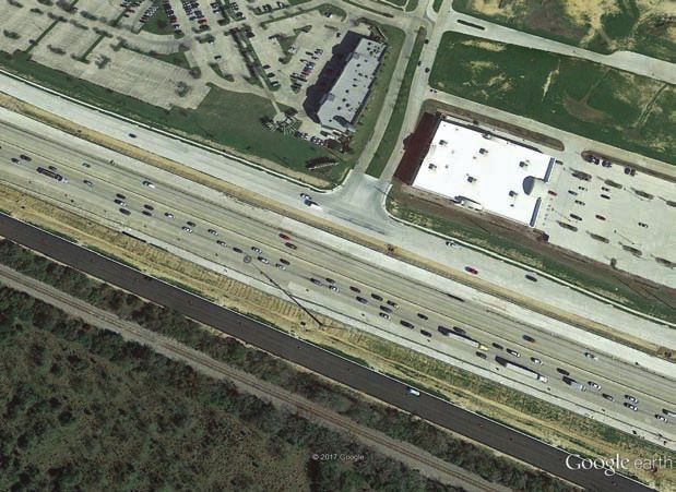
Geophysics of the Hockley Fault in Texas 3
data on the downthrown and upthrown sides of the faults, including all figures in this paper for georeferencing purposes. The location
geophysical logs and core data along with borehole data (Elsbury of the F1254 marker is 29°59′34″N latitude and 95°45′17″ west
et al., 1980). longitude.
Pioneering resistivity work was performed over some of the Hous- The Hockley Fault initiates at the Hockley salt dome (Figure 2),
ton faults by Kreitler and McKalips (1978). They use a resistivity and it trends in the northeast–southwest direction. The trend of the
meter with four electrodes and conduct resistivity surveys over sev- fault shifts to the east approximately 150 m south of Highway 290
eral fault locations using a Wenner array. Their results identified (see the southeast location on the map in Figure 3b of Khan et al.
anomalous resistivity values that correlated with
the locations of the faults. Years later, these resis-
tivity results prompted one of the authors of this
paper (M. Saribudak) to use a multielectrode re-
Premium Outlet Shopping Mall
29°59'40"N
sistivity meter and other geophysical methods Approximate location
of fault trace from Khan
(conductivity, magnetic, gravity, and GPR) across et al. (2013)
the Willow Creek growth fault. All five geophysi-
cal methods were used to map and characterize the
Willow Creek Fault. All provided consistent R4 U
D
anomalies over the fault (Saribudak and Van Nieu-
wenhuise, 2006). Engelkemeir and Khan (2007)
U
D
publish seismic and GPR data over the Long Point R2
Fault, which is one of the most destructive active
29°59'35"N
faults in the Houston area. More resistivity sur- M R1
veys were conducted over the Long Point, G
C
Katy-Hockley, Tomball, and Pearland Faults, and
results were published in Saribudak (2011b). Dur- NSRS F1254
R3
ing the same year, integrated geophysical results
(resistivity and GPR) were published in Saribudak
M Magnetic Fault locations based
(2011a) for the Hockley Fault. More recently, R Resistivity on faults, scarps, and
resistivity anomaly
Khan et al. (2013) publish geophysical results G Gravity
0 30 m
C Conductivity
(seismic, gravity, and GPR), which were collected
95°45'15"W 95°45'10"W
after the construction of the shopping center and
expansion of Highway 290, over the Hockley Figure 3. Site map showing the locations of magnetics (M), conductivity (C), and grav-
Fault along with airborne LiDAR data of 2001 ity (G) profiles. Locations of resistivity profiles (R1–R4) and fault scarps were taken
and 2008. from Saribudak (2011a). Note that the site map also shows the approximate trend of the
Hockley Fault trace (dashed white line) interpreted by Khan et al. (2013), which
obliquely crosses Highway 290.
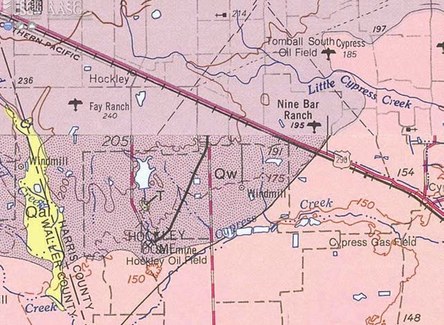
GEOLOGY OF THE HOCKLEY
FAULT AT HIGHWAY 290
Figure 4 shows the general geology of the
study area and stratigraphy of Harris County Lissie Fm
(Bureau of Economic Geology, 1992). In gen- Willis Fm
eral, the Willis Formation underlies the Lissie Willis Fm
Formation stratigraphically. Both of these Pleis-
tocene sedimentary formations are entirely non-
marine and a series of incised stream valleys
interspersed with deposits of deltas and flood-
plains (Ewing, 2016). The Willis Formation is
composed of clays with lesser amounts of silts NSRS F1254
and sands. The Lissie Formation mainly contains Willis
Fm
sands with fewer silts and clays (Bureau of U
D
Economic Geology, 1992). According to the geo-
logic map, the Hockley Fault lies at the contact of
these two formations: on the upthrown side, the Hockley
Fault Lissie Fm
Willis Formation, and on the downthrown side, Lissie Fm
the Lissie Formation. The National Reference
System (NSRS) has a survey marker on the 0 5 km
downthrown side of the fault, which is identified
as F1254. We found no specific information in
Figure 4. A geologic map of the Hockley Fault study area showing the Willis and Lissie
the NSRS database for marker F1254 regarding Formations (taken from Bureau of Economic Geology, 1992). The older Willis Forma-
the evolution of the Hockley Fault. We noted the tion underlies the Lissie Formation. Note the location of NSRS survey marker F1254 at
location of this survey marker, and it is shown in the Hockley Fault.
4                                                                Saribudak et al.

[2013] and Figure 13 in this paper). Then, the fault crosses                to 28 mS∕m across the fault (Figure 5). The cause of the conduc-
obliquely to the north of Highway 290, adjacent to a newly built            tivity anomaly is likely to be the Hockley Fault.
shopping center, as interpreted by Khan et al. (2013).
                                                                                                   MAGNETIC DATA

                           CONDUCTIVITY DATA                                   A Geometrics G-858 Cesium magnetometer was used to acquire
                                                                            the data. It measures the total magnetic field in units of nT.
   We used a Geonics EM31 conductivity meter to conduct the                 The collection rate of the magnetic data was such that the spacing
electromagnetic survey. The maximum depth exploration of this               between the data points was less than 0.5 m along the magnetic
meter is approximately 6 m. The EM31 meter measures the appar-              profile. The length of the profile was 122 m, and the magnetic data
ent conductivity of soil. The data were collected in vertical dipole        were acquired along profile M (Figure 3). A base station was es-
mode, and its unit is miliSiemen/meter (mS∕m). The collection rate          tablished in the vicinity of the site to record the daily variations
of the conductivity data was such that the spacing between the data         of the earth’s external magnetic field. The magnetic survey time
points was less than 0.5 m along the profile. The length of the pro-        was less than 30 min, and there were no significant diurnal varia-
file was 190 m.                                                             tions. For this reason, a diurnal correction was not applied to the
   Figure 5 shows the conductivity data. Conductivity values start          magnetic data.
at 27 mS∕m at the west end of the profile and increase steadily to             A low-pass filter was applied to the magnetic data to reduce
the southeast. The maximum value of 38 mS∕m is attained between             noise. The filtered profile is shown in Figure 6. The magnetic data
65 and 100 m along the traverse and decreases to 28 mS∕m with a             were not reduced to pole (RTP). We advise against application of
sharp slope at the Hockley Fault and continues to fluctuate between         the RTP to a single profile (unless it is a truly north–south profile).
28 and 31 mS∕m for the rest of the profile (see Figure 5). The con-         For the RTP filter to properly shift the total magnetic intensity
ductivity data represent a fault-like signature over the Hockley            (TMI) anomaly to its correct reduced-to-pole position, 2D, or
Fault. Unconsolidated sediments with conductivity values between            map-based information about the complete TMI dipole is required.
27 and 38 mS∕m are generally attributed to silts and sands (Kress           At our survey location, TMI data along a single profile oriented
and Teeple, 2003). These appear to be prevalent on both sides of            northwest to southeast are not sufficient to correctly map an RTP
the fault.                                                                  anomaly in its proper location. The average magnetic anomaly is
   The NSRS survey marker F1254 is located near station 152 m               48,625 nT between stations 0 and 46 m in the upthrown section of
(Figure 5), 52 m southeast of the fault location. The conductivity          the fault. The magnetic values drop to 48,475 nT between
traverse overlaps a portion of the resistivity profile R1 (see Fig-         stations 46 and 58 m, creating a significant low magnetic anomaly.
ures 3). The resistivity data show relatively low-resistivity (high         The magnetic values then increase up to 48,575 nT for the rest of
conductivity) values of 24 Ωm on the upthrown side of the fault             the profile. The magnetic profile indicates slightly more positive
as deep as 10 m. However, relatively high-resistivity values, up            magnetic values on the upthrown side of the fault with respect to
to 50 Ωm (low conductivity), are imaged over the downthrown side            the downthrown side and a region of relatively low magnetic in-
of the fault. In fact, the conductivity values drop sharply from a 38       tensity in the vicinity of the fault. The source of this negative
                                                                                               anomaly could be the alteration of magnetic
                                                                                               minerals in the fault zone. The Willis and Lissie
                                                                    NSRS                       Formations contain iron oxide and iron-manga-
         Northwest                        Location of fault         F1254        Southeast     nese nodules (Bureau of Economic Geology,
   38.00
   36.00                                                                                       1992). The magnetic profile images a fault sig-
                                                                                               nature, and it is likely caused by the Hock-
mS/m

   34.00
   32.00
                                                                                               ley Fault.
   30.00
   28.00                                                                                          It should be mentioned that a significant and
        0          30.4         61.0         91.5        122.0       152.0        183.0
                                                                                               well-defined relative negative magnetic anomaly
                                                 m                                             was obtained over the downthrown section of the
                                                                                               Willow Creek Fault (see Figure 7a in Saribudak
Figure 5. Conductivity anomaly indicating the location of the Hockley Fault. The               and Van Nieuwenhuise, 2006), and it is very sim-
location of the fault is consistent with the results of Khan et al. (2013).                    ilar to the magnetic anomaly obtained over the
                                                                                               Hockley Fault.
                                                                                                  The locations of the Hockley Fault and the
                                                                       NSRS                    NSRS survey marker F1254 are shown as refer-
                                  Location of fault                    F1254 Southeast         ences on the profile. Their separation distance is
            Northwest
   48650.00
                                                                                               53 m. Note that the distances between fault loca-
nanoTesla

   48600.00
   48550.00                                                                                    tions on the conductivity and magnetic profiles
   48500.00                                                                                    and the survey marker are similar.
            48450.00

                       0   15.2   30.5   45.7   61.0
                                                 m
                                                          76.2       91.5     106.7     122.0
                                                                                                              GRAVITY DATA

Figure 6. Magnetic anomaly indicating the location of the Hockley Fault. The magnetic              The gravity data were acquired using a La-
expression of the fault correlates well with the conductivity data. The location of the         Coste & Romberg G-Meter, SN-670. The length
fault is consistent with the results of Khan et al. (2013).                                     of the profile was 275 m. The units are in mGal.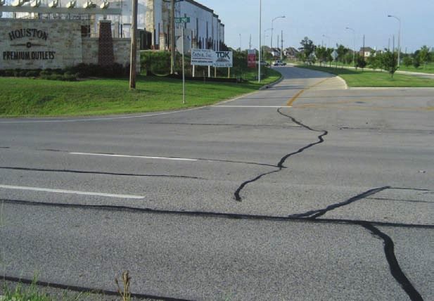
Geophysics of the Hockley Fault in Texas                                                                                                                        5

Gravity stations were precisely located along the profile G (see Fig-                              RESISTIVITY DATA
ure 3). A base station was established, and it was reoccupied three
times during the survey. In addition, the data were tied to two grav-            Resistivity data (profiles R1, R2, R3, and R4) are presented in
ity base stations: one at the Willow Creek site (Saribudak and Van           Saribudak    (2011a) to emphasize an important point. Resistivity pro-
Nieuwenhuise, 2006) and one at an intermediary location in Spring,           file R1 is aligned with the conductivity, magnetic, and gravity pro-
Texas. This allowed for rapid reoccupation of gravity base stations          files of this study and Khan et al. (2013); but the R2 and R3 profiles
and increased gravity data repeatability (
6                                                                Saribudak et al.

R4 run parallel. Resistivity profile R3 overlaps profile R2 along its       geophysical results of Khan et al. (2013), thus corroborating a
eastern extent (Figure 3). Note that resistivity profile R4 is located      common location of the fault.
on the northern part of Highway 290 (Figure 3).                                A similar fault anomaly is observed on resistivity profile R3,
   The quality of the resistivity data obtained across the site is ex-      which is located further north of profile R1 and offset to the east
cellent. There were no noise sources along the resistivity profiles,        by 50 m (Figure 8). The same fault-like anomaly is observed on
such as power lines and buried utility lines. The statistical values of     resistivity profile R2 and R4, north across Highway 290 (see also
the inverted resistivity data (L1–L4) are shown on each profile with        the resistivity profiles of L5, L6, and L7 in Figures 3, 6, and 7 of
root-mean-square (rms) and L2 (normalized) parameters, which are            Saribudak [2011a]).
in the range of 3 and 7, and 0.77 and 0.96, respectively (Figure 8).           Note that the fault trace (the dashed black line in Figure 8) de-
These values are excellent and indicate the presence of noise-free          termined by Khan et al. (2013) crosses not only resistivity profile
data and reliable inversion.                                                R1, but also R2 and R4. However, our resistivity data for both the
   Resistivity profile R1 indicates a fault-like anomaly at around          R2 and R4 traverses does not indicate the presence of any fault
station 90 m at the boundary between high- and low-resistivity              anomaly where Khan et al.’s. (2013) interpreted fault trace is shown
units (Figure 8). In the upthrown section of the fault, relatively low-     (Figure 8).
resistivity values are observed in the depth of first 5 m of the subsur-       The geologic map (Figure 4) shows the Willis Formation (mainly
face (approximately 24 Ωm), whereas in the downthrown section               clay) on the upthrown side and the Lissie Formation (mainly sand)
of the fault, relatively higher resistivity values are observed (up         on the downthrown side of the Hockley Fault. The resistivity data
to 55 Ωm). This observation correlates well with the conductivity           indicate that the main lithologic unit is sand, which is observed at
data, because the depth penetration of EM31 conductivity unit is not        depths of 15–40 m. In the resistivity section, a 10 m layer of low-
more than a few meters in the conductive environment. The resis-            resistivity (clay and silt) section overlies the sand unit. Detailed
tivity profile displays a chaotic mixture of low-resistivity values in      review of the geologic map and the report indicates that sand units
the downthrown section. This is probably due to the fault deforma-          could be the channel facies of the Willis Formation (Bureau of Eco-
tion that has taken place within the Hockley Fault zone.                    nomic Geology, 1992).
   This anomalous fault location correlates well with our fault lo-
cations mapped from conductivity, gravity, and magnetics and the                                    GRAVITY AND MAGNETIC
                                                                                                          MODELING
                                                                                                 Our nonunique model of the unfiltered gravity
                                                                                              and magnetic data (Figure 9) shows a strong cor-
                                                                                              relation of a lateral change in the magnetic and
                                                                                              density properties of the Hockley Fault. The depth
                                                                                              model, in the lower panel of Figure 9, ranges from
                                                                                              100 m above sea level to 100 m below sea level.
                                                                                              The location of the fault is shown in red. The
                                                                                              central panel shows the observed gravity and com-
                                                                                              puted gravity response of the model, and the upper
                                                                                              panel shows the observed magnetics signal and
                                                                                              computed magnetics response of the model. The
                                                                                              surface location of the Hockley Fault is shown as
                                                                                              the red arrows (Figures 9 and 10).
                                                                                                 We modeled the gravity and magnetic data
                                                                                              using 2D forward-modeling software (Geosoft
                                                                                              Oasis Montaj GMSYS2D). We iteratively modi-
                                                                                              fied the structure and physical properties (density
                                                                                              and magnetic susceptibility) of the model until
                                                                                              the computed response matched the observed
                                                                                              signal. Based on resistivity modeling, we already
                                                                                              had a general concept of the fault geometry. We
                                                                                              used this for the structural constraint in modeling
                                                                                              the gravity and magnetics data.
                                                                                                 Our proposed model, color coded by density,
                                                                                              is shown in Figure 9. It images a low-density
                                                                                              zone of unconsolidated sediments (colored in
                                                                                              blue) at the location of the fault. We interpreted
                                                                                              this as a low-density fault zone, which is possibly
                                                                                              very saturated. To the southeast, we see a high-
                                                                                              density block of the downthrown Lissee Forma-
Figure 9. Modeling of gravity data. The letter D denotes the density of the unconsoli-
dated sediments in the near surface. See the text for explanation. Note the presence of the   tion. This density (2.4) is high, considering the
low-density zone shown by the blue strip adjacent to the fault location. The red arrow        depth of unit; but it is possibly due to differential
indicates the location of the Hockley Fault.                                                  compaction, which is a diagenetic process that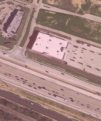
Geophysics of the Hockley Fault in Texas                                                          7

begins during burial and may continue through-
out burial and/or the duration of the growth fault.
Compaction increases the bulk density and com-
petence of rock, whereas it reduces porosity
(Hooper, 1991). Compaction curves obtained
from indicate that sediments whose densities
are 2.0 g∕cm3 near the surface may experience
an increase in their density of up to 2.6 g∕cm3
with compaction.
   In addition, during our geophysical surveys at
the Hockley and Willow Creek faults, we (Bob
and Mustafa) observed that downthrown sides of
the faults ponded rainwater for long periods of
time after heavy rainfalls. We believe that the
downthrown sediments were perhaps even denser
than the upthrown sediments due to their satura-
tion (https://www.engineeringtoolbox.com/dirt-
mud-densities-1727.html).
   Figure 10 shows the same model, color coded
by magnetic susceptibility. The only magnetic
source we have placed in the model is the narrow
zone of anomalously magnetized material near
the fault. The source of this magnetization could
be due to the alteration of mineralogies by intro-
duction of fluids into the fault zone. There is a
substantial body of data regarding the impor-
tance of fault zones as conduits of vertical fluid
migration in sediments (Losh et al., 1999;
Kuecher et al., 2001). Evidence for growth faults
as avenues of fluid migration includes fault-zone      Figure 10. Modeling of magnetic data. The red arrow indicates the Hockley Fault lo-
mineralization, thermal anomalies, and salinity        cation. The yellow strip corresponds to the low magnetic anomaly, which is interpreted
anomalies (Hooper, 1991).                              to be the narrow zone of anomalously magnetized material along the fault. The magnetic
   The modeled low magnetic anomaly due to the         data were modeled using a 10 m low-pass filter.
mineralized fault zone corresponds to the gravity
anomaly low in density. This observation is puz-
zling, and we look forward to possibly observing
this relationship in other fault zones.                                           Premium Outlet Shopping Mall
                                                       29°59'40"N

   Parameters used in the magnetic modeling are
as follows: M is the magnetization of the rema-
nence, units are micro-EMU∕cm3 ; S is the mag-
netic susceptibility, units are micro-CGS; MI is the
inclination of the remanence in degrees; and MD                     Sand layers with high resistivity
is the declination of the remanence in degrees.
                                                                                                               U
                                                                                                              D

                DISCUSSION                                                                                     Sand layers with low resistivity
                                                       29°59'35"N

   Data from four geophysical methods were                                       A
used to image the Hockley Fault where it crosses
                                                                                 U
                                                                                D

Highway 290 in Cypress, Texas. The conduc-                                           NSRS
tivity data display a typical fault anomaly with                                 survey marker
a steep slope over the fault location. The mag-                                      F1254         Chaotic mixture of
netic data also present a fault-like anomaly. Rel-                                                  sand layers with
                                                                      Fault locations based         low resisistivity
atively high magnetic values are associated with                      on faults, scarps, and
                                                                      resistivity anomaly
the upthrown side, and relatively low magnetic                            0          30 m
values are on the downthrown side. The source
of the magnetization is modeled to be the narrow                                                 95°45'15"W                  95°45'10"W

zone of anomalously magnetized material near
                                                       Figure 11. Schematic map showing near-surface lithologies and the shift of the Hockley
the fault location. The gravity data differ from       Fault across Highway 290 based on the resistivity data from Saribudak (2011a) and this
the conventional case. A gravity high is observed      study. The letter A designates the location where this study and Khan et al. (2013) ob-
on the downthrown side of the fault. It is prob-       tained similar fault anomalies.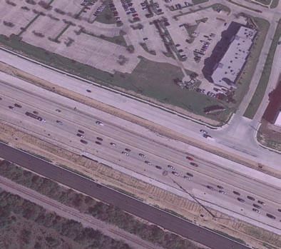
8 Saribudak et al.
ably caused by compaction and high saturation of the unconsoli- Locations of the fault based on the resistivity data (Saribudak,
dated sediments in the downthrown side. We successfully model 2011a) and the data obtained from this study are marked on a site
this response using slightly higher density values on the down- map (Figure 11). The common fault location determined by this
thrown part of the fault. study and Khan et al. (2013) is marked with a letter A (yellow color)
Results of seismic, GPR, and gravity from Khan et al. (2013) also on the southern part of Highway 290. However, fault-like anomalies
obtained a fault anomaly at the same location of this study. Their obtained from the resistivity data and visible fault scarps
gravity profile indicated a similar gravity anomaly (higher readings indicate that the fault shifts to the east as it crosses north of
on the downthrown side) across the Hockley Fault. It should be Highway 290.
noted that the amplitude (approximately 0.3 mGal) and wavelength The geologic units identified by the resistivity data are also
(225 m) of the fault’s gravity anomaly of Khan et al. (2013) corre- shown in Figure 11. The resistivity data in this area indicate a cha-
late well with this study, which are approximately 0.25 mGal and otic mixture of sand and silt units, which are probably caused by
270 m, respectively. the fault zone between the two main branches of the Hockley Fault.
The width of the fault zone is estimated to be
approximately 65 m.
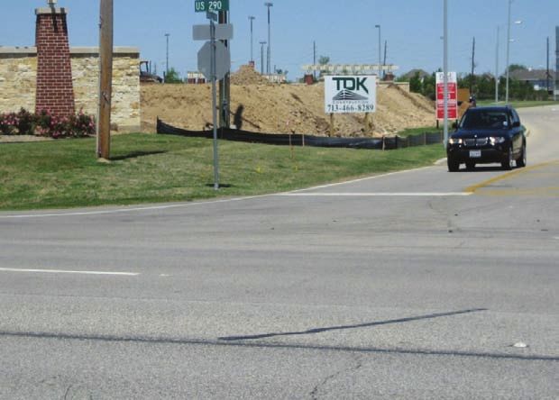
After the completion of our geophysical
surveys, a shopping mall was built in the vicin-
a) ity of the Hockley Fault. Highway 290 was
April 2010 rebuilt and extended, covering the fault outcrop.
A site visit during April 2010 did not show any
significant deformation across a newly built
road. However, three months later, during our
August 2010 site visit, we observed large
cracks in the pavement along the fault trace
(Figure 12).
A similar observation was noted when we
studied two Google images of the study area
from 2004 and 2017 (Figure 13). The 2004 im-
age indicates a dark patch on the northern section
of Highway 290. This asphalt patch covers the
fault scarp and deformation on the highway at
this location. However, the 2017 image did not
N include the patch or any related fault deforma-
tion. We precisely mapped the location of the
2004 fault patch on the 2017 Google image.
In addition, we also mapped the fault trace accu-
rately determined by Khan et al. (2013) onto the
b) 2017 image. One can easily observe that the
August 2010
2004 fault patch is located approximately 30 m
to the east of the Khan et al. (2013) fault trace.
Figure 13 shows the future location of the Outlet
Shopping Mall and Highway 290 for reference
purposes.
A 2008 LiDAR data set of the Hockley Fault
area, which is publicly available, is shown in
Figure 14. We show the trend of the Hockley
Fault with small black and white arrows. At
location A, the LiDAR data display the fault
trace well on the north and south sides of High-
way 290, with a visible shift, to the fault trend.
However, the LiDAR data do not show any trace
of the fault on Highway 290. As it appears, the
N
Hockley fault deformation trend of the fault also shifts eastward at location
B on Highway 290 (Figure 14). This observation
suggests that the shifting of the main Hockley
Fault along its strike is an active feature. One
can visit the discrete fault line and observe the
Figure 12. (a) Newly paved asphalt has been placed over the Hockley Fault in April
2010 at the entrance road of the shopping center. Note that this part of the mall was still ongoing fault deformation across the newly built
under construction at that time; (b) the fault deformation manifested itself within three Highway 290 as outlined in this geophysical
months, and cracks were patched with black asphalt. study.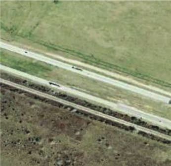
Geophysics of the Hockley Fault in Texas                                                 9

a)                                                                                       2004        Figure 13. Google images of 2004 and 2017:
                                                                                                     (a) A patch on the asphalt covers the fault scarp
                                Future Shopping Mall                                                 and fault deformation on Highway 290 in the year
                                                                                                     2004; (b) the location of the 2004 patch is plotted
                                                                                                     on the 2017 Goggle image. The fault trace ob-
                                                                                                     tained by Khan et al. (2013) is also shown on
                                                                                                     the site map.

                                                                      Fault
                                                                      patch

         0           15 m

b)
                                                                                         2017
                                Premium Outlet
                                Shopping Mall
                                               U
                                                     D

                                                                Fault patch

                                Approximate location of
                                fault trace by Khan et al., 2013
                            0                 15 m

                                                                                         Elevation   Figure 14. A LiDAR map showing the Hockley
         N                                                                                  (m)
                                                                                                     Fault location in the vicinity of the study area.
                                                                                              60.0   The white and black arrows indicate the fault trace
                                                                                                     at locations A and B, respectively.
                                                                                              57.5
                                            Future
                                     Outlet Shopping Mall                                     55.0
                                US
                                     Hig
                                        hwa
                                           y2                                                 52.5
                                                90

                                                         A                                    50.0

                                                                                              47.5
                                                                          To
                                                                               Hou
                                                                                  sto
                                                                                     n
                                                                                              45.0
                                           B
     0       150 m
                                                                                              42.5
                                                                                              41.1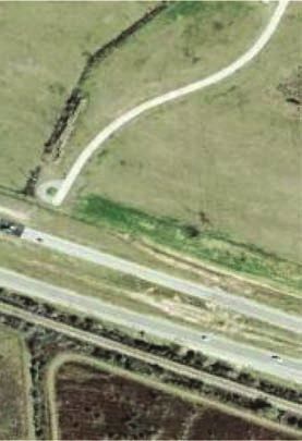
10                                                                   Saribudak et al.

                           CONCLUSION                                          Engelkemeir, R., and S. D. Khan, 2007, Near-surface geophysical studies of
                                                                                 Houston faults: The Leading Edge, 26, 1004–1008, doi: 10.1190/1
                                                                                 .2769557.
   The Hockley Fault was investigated in detail with a variety of geo-         Ewing, T., 2016, Texas through time: Lone star geology, landscapes and
physical methods. Magnetic, conductivity, and gravity data imaged a              resources: Bureau of Economic Geology, Udden Series 6.
fault signature across the structure in the southern portion of the study      Ewing, T. E., 1983, Growth faults and salt tectonics in the Houston diaper
                                                                                 province: Relative timing and exploration significance: Transactions of
area. Two-dimensional resistivity data provided useful information               the 33rd Annual Meeting of the Gulf Coast Association of Geological
for identifying the lithologies from the surface to 40 m depth. In ad-           Societies, 83–90.
                                                                               Hooper, E. C. D., 1991, Fluid migration along growth faults in compacting
dition, the resistivity data acquired on the south and north of Highway          sediments: Journal of Petroleum Geology, 14, 161–180, doi: 10.1111/j
290 suggest an easterly shift on the trace of the Hockley Fault. This            .1747-5457.1991.tb00360.x.
interpretation is supported by publicly available LiDAR data and our           Kasmarek, C. M., and W. E. Strom, 2002, Hydrogeology and simulation of
                                                                                 ground-water flow and land surface subsidence in the Chicot and Evan-
observations of surface deformation across the study area.                       geline aquifers, Houston, Texas: U.S. Geological Survey, Water-Resour-
   New modeling of gravity and magnetic data over the fault, using               ces Investigations Report 02-4022.
resistivity models for constraint, was performed. The nonunique                Khan, S. D., R. R. Stewart, M. Otoum, and L. Chang, 2013, A geophysical
                                                                                 investigation of the active Hockley fault system near Houston, Texas:
model of the gravity and magnetic data shows the strong correlation              Geophysics, 78, no. 4, B177–B185, doi: 10.1190/geo2012-0258.1.
of a lateral change in density and magnetic properties across the              Kreitler, C., and D. McKalips, 1978, Identification of surface faults by hori-
                                                                                 zontal resistivity profiles, Texas coastal zone: Bureau of Economic Geol-
Hockley Fault.                                                                   ogy, Geological Circular 78-6.
                                                                               Kress, H. W., and P. A. Teeple, 2003, Two-dimensional resistivity investi-
                                                                                 gation of the north Cavalcade Street site, Houston, Texas: USGS Scien-
                    ACKNOWLEDGMENTS                                              tific Investigation Report 2005-5205.
                                                                               Kuecher, G. J., S. S. Roberts, M. D. Thompson, and I. Matthews, 2001,
   Bob Van Nieuwenhuise, the coauthor of this paper, helped to                   Evidence for active growth faulting in the Terrebonne Delta Plain, South
collect the geophysical data during the years of 2004 and 2005.                  Louisiana: Implications for wetland loss and the vertical migration of
                                                                                 petroleum, AAPG/DEG: Environmental Geosciences, 8, 77–94, doi:
He passed away in 21 September 2014. He would have loved to                      10.1046/j.1526-0984.2001.82001.x.
have seen this paper published. He was a good friend, a colleague,             Losh, S., L. Eglinton, M. Schoell, and J. Wood, 1999, Vertical and lateral
and enthusiastic about his work. He loved geophysics and geology.                fluid flow related to a large growth fault, South Eugene Island Block 330
                                                                                 Field, offshore Louisiana: The AAPG Bulletin, 83, 244–276.
We dedicate this work to Bob. This research project was born out of            O’Neill, M. W., and D. C. Van Siclen, 1984, Activation of Gulf Coast faults
personal curiosity and was supported by the authors’ financial com-              by depressuring of aquifers and an engineering approach to siting struc-
                                                                                 tures along their traces: Bulletin — Association of Engineering Geol-
mitment and/or their time. We thank J. Jardon, our graphic designer,             ogists, 21, 73–87.
who designed and drew the figures.                                             Paine, J., 1993, Subsidence of the Texas coast: Inferences from historical and
   Special thanks to geologist A. Grubb for obtaining and delivering             Late Pleistocene sea levels: Tectonophysics, 222, 445–458, doi: 10.1016/
                                                                                 0040-1951(93)90363-O.
the LiDAR data to us and D. Van Nieuwenhuise of the University of              Saribudak, M., 2011a, Geophysical mapping of the Hockley growth fault in
Houston for reviewing the manuscript. Finally, we appreciate J.                  northwest Houston, USA, and recent surface observations: The Leading
Paine of the Bureau of Economic Geology for his careful review                   Edge, 30, 172–180, doi: 10.1190/1.3555328.
                                                                               Saribudak, M., 2011b, 2D resistivity imaging investigation of long point,
of the manuscript and his insightful input.                                      Katy-Hockley, Tomball and Pearland Faults, Houston, Texas: Houston
   We acknowledge the anonymous reviewers for their reviews,                     Geological Society, 54, 39–48.
which greatly improved the content and flow of the paper.                      Saribudak, M., and B. Van Nieuwenhuise, 2006, Integrated geophysical
                                                                                 studies over an active growth fault in Houston: The Leading Edge, 25,
                                                                                 332–334, doi: 10.1190/1.2184101.
                                                                               Sheets, M. M., 1971, Active surface faulting in the Houston area, Texas:
                           REFERENCES                                            Houston Geological Society Bulletin, 13, 24–33.
                                                                               Shelton, J., 1984, Listric normal faults: An illustrated summary: AAPG Bul-
Bureau of Economic Geology, 1992, Geologic map of Texas: University of           letin, 68, 801–815.
  Texas at Austin, Virgil E. Barnes, project supervisor, Hartmann, B. M.,      Verbeek, E. R., 1979, Surface faults in the Gulf coastal plain between Vic-
  and D. F. Scranton, cartography, scale 1:500,000.                              toria and Beaumont, Texas: Tectonophysics, 52, 373–375, doi: 10.1016/
Clanton, U. S., and D. L. Amsbury, 1975, Active faults in southeastern           0040-1951(79)90248-8.
  Harris County, Texas: Environmental Geology, 1, 149–154, doi: 10             Verbeek, E. R., and U. S. Clanton, 1978, Map showing faults in the
  .1007/BF02428942.                                                              southeastern Houston metropolitan area, Texas: U.S. Geological Survey
Clanton, U. S., and R. E. Verbeek, 1981, Photographic portraits of active        Open File Report 78–79.
  faults in the Houston metropolitan area, Texas, in M. E. Etter, ed., Hous-   Verbeek, E. R., and U. S. Clanton, 1981, Historically active faults in the
  ton area environmental geology: Surface faulting, ground subsidence,           Houston metropolitan area, Texas, in M. E. Etter, ed., Houston area envi-
  hazard liability: Houston Geological Society, 70–113.                          ronmental geology: Surface faulting, ground subsidence, hazard liability:
Elsbury, B. R., D. C. Van Siclen, and B. P. Marshall, 1980, Engineering          Houston Geological Society, 28–69.
  aspects of the Houston fault problem: ASCE Fall Meeting.
You can also read