Improving Low Earth Orbit (LEO) Prediction with Accelerometer Data - MDPI
←
→
Page content transcription
If your browser does not render page correctly, please read the page content below
remote sensing
Article
Improving Low Earth Orbit (LEO) Prediction with
Accelerometer Data
Haibo Ge 1,2 , Bofeng Li 1, * , Maorong Ge 2,3 , Liangwei Nie 2,3 and Harald Schuh 2,3
 1    College of Surveying and Geo-Informatics, Tongji University, Shanghai 200092, China;
      haibo.ge@gfz-potsdam.de
 2    Department of Geodesy, GeoForschungsZentrum (GFZ), Telegrafenberg, 14473 Potsdam, Germany;
      maorong.ge@gfz-potsdam.de (M.G.); liangwei@gfz-potsdam.de (L.N.); schuh@gfz-potsdam.de (H.S.)
 3    Institut für Geodäsie und Geoinformationstechnik, Technische Universität, 10963 Berlin, Germany
 *    Correspondence: bofeng_li@tongji.edu.cn

 Received: 10 April 2020; Accepted: 15 May 2020; Published: 17 May 2020

 Abstract: Low Earth Orbit (LEO) satellites have been widely used in scientific fields or commercial
 applications in recent decades. The demands of the real time scientific research or real time applications
 require real time precise LEO orbits. Usually, the predicted orbit is one of the solutions for real time
 users, so it is of great importance to investigate LEO orbit prediction for users who need real time
 LEO orbits. The centimeter level precision orbit is needed for high precision applications. Aiming at
 obtaining the predicted LEO orbit with centimeter precision, this article demonstrates the traditional
 method to conduct orbit prediction and put forward an idea of LEO orbit prediction by using onboard
 accelerometer data for real time applications. The procedure of LEO orbit prediction is proposed
 after comparing three different estimation strategies of retrieving initial conditions and dynamic
 parameters. Three strategies are estimating empirical coefficients every one cycle per revolution,
 which is the traditional method, estimating calibration parameters of one bias of accelerometer hourly
 for each direction by using accelerometer data, and estimating calibration parameters of one bias
 and one scale factor of the accelerometer for each direction with one arc by using accelerometer data.
 The results show that the predicted LEO orbit precision by using the traditional method can reach
 10 cm when the predicted time is shorter than 20 min, while the predicted LEO orbit with better than
 5 cm for each orbit direction can be achieved with accelerometer data even to predict one hour.

 Keywords: Low Earth Orbit (LEO); orbit prediction; accelerometer data; calibration parameters;
 empirical coefficient; initial conditions; dynamic parameters

1. Introduction
      More and more Low Earth Orbit (LEO) satellites have been launched to explore various phenomena
on Earth [1,2], e.g., ocean altimetry [3,4], climate change, and Earth mass change [5]. In recent years,
many research plans or commercial projects depending on a large number of LEO satellites have been
proposed with the expectation of providing real time services on a global scale [6–8]. Meanwhile,
the idea of a LEO enhanced Global Navigation Satellite System (LeGNSS) [9,10], where LEO satellites
will transmit navigation signals to be used as navigation satellites, was put forward with such a large
number of LEO satellites. With such a huge demand of real time services and different kinds of real
time applications, especially for the real time Precise Point Positioning (PPP) of LeGNSS, real time
centimeter level LEO orbits are the prerequisite for real time users. Near real time LEO orbits are
provided for the fields of satellite occultation for meteorological purposes [11,12] and the short-latency
monitoring of continental, ocean, and atmospheric mass variations [13,14]. The European Space
Agency (ESA) has deployed an operational system for routine Earth Observation named Copernicus

Remote Sens. 2020, 12, 1599; doi:10.3390/rs12101599                       www.mdpi.com/journal/remotesensing
Remote Sens. 2020, 12, 1599                                                                           2 of 18

since 2014, which is designed to support a sustainable European information network by monitoring,
recording, and analyzing environmental data and events around the globe [15]. The Copernicus
program consists of six different families of satellites being the first three missions Sentinel -1, -2, and
-3. These missions have the requirements of 8-10 cm in less than 30 min for Near Real Time (NRT)
applications to 2-3 cm in less than one month for Non-Time Critical (NTC) applications [16]. The orbit
accuracy of Sentinel-2A NRT products is better than 5 cm, which is better than the requirement of
10 cm as well as better than the accuracy of previous NRT LEO orbits studies [17,18]. Though the
accuracy of the NRT orbit is on the centimeter level, the latency of about 30 min is not acceptable for
real time positioning service of LeGNSS. Thus, predicted LEO orbit with centimeter precision should
be investigated. In this study, we try to find a proper way to conduct the prediction of LEO orbits with
an orbit precision on the centimeter level for real time applications, especially for the case of LeGNSS.
      In order to obtain such highly accurate predicted LEO orbit for precise real time applications,
precise initial conditions (position and velocity at reference time) as well as the dynamic parameters
of LEO satellites used for LEO orbit prediction are required as fast as possible via LEO Precise Orbit
Determination (POD). Thus, standard GNSS navigation message information is not adequate for LEO
POD since the qualities of GNSS orbits and clocks are not good enough. The precision of the LEO
orbit is usually at the decimeter or meter level by using the standard GNSS navigation message [12,19].
Under this circumstance, precise GNSS products should be used for LEO POD in order to get precise
initial conditions and dynamic parameters of LEO satellites. Due to the Real Time Pilot Project (RTPP)
launched by the International GNSS Service (IGS) in 2007 and officially operated since 2012 [20],
real time precise satellite orbit and clock correction products can be obtained with Real Time Service
(RTS). Currently, there are also many commercial providers, which deliver real time GPS/GNSS orbit
and clock correction products, e.g., Veripos, magicGNSS, etc. Obviously, RTS can be applied to LEO
POD both in the kinematic and dynamic mode. However, most onboard LEO receivers have not yet
used these corrections, as it might not yet be mature enough for space applications. An alternative way
is to conduct LEO POD at the analysis center with the RTS on the ground with powerful computational
resources. As for the POD mode, though either kinematic or dynamic POD can achieve centimeter level
orbit precision, we prefer to choose the dynamic method since the orbit of this method is consecutive
and stable while that of the kinematic method is discrete. Above all, we conduct dynamic orbit
determination, which estimates LEO initial conditions and dynamic parameters with real time precise
GNSS orbit and clock products. Then, these dynamic parameters and initial conditions are used to do
the orbit integration for times in the future, referred as orbit prediction.
      Here, two issues should be taken into consideration. The first one is the update rate of the precise
LEO orbit. The update rate of the LEO orbit depends on the time gap of LEO onboard observation
data collection as well as the calculation time of LEO POD. The LEO onboard observations cannot
be transferred to the ground stations all the time and the LEO orbit results calculated at an analysis
center cannot be always uploaded to the LEO satellites unless the LEO satellites fly over the uplink
and downlink stations. It is reasonable to assume that the onboard data can be collected every
one hour (more than half LEO orbit revolution, personal communication with Xiangguang Meng,
who is in charge of Chinese FY3C near real time POD). The second issue is the length of the orbit
prediction. An empirical force model with parameters is usually utilized in dynamic LEO precise orbit
determination to absorb the unmodeled part of non-gravitational forces, such as atmosphere drag and
solar radiation pressure [21–24]. These parameters are important for the precision of orbit prediction if
they fit the real characteristics of the unmodeled part of non-gravitational forces for the prediction arc.
      Currently, some LEO satellites carry accelerometers to measure non-gravitational accelerations
due to the surface forces acting on the LEO satellites, such as STAR instrument on Challenging
Minisatellite Payload (CHAMP), SuperSTAR instruments on Gravity Recovery and Climate Experiment
(GRACE), and GRADIO instruments on the Gravity field and steady-state Ocean Circulation
Explorer (GOCE).    √ These instruments √ have extreme sensitivity
                                                               √      and unprecedented accuracy with
up to 10−9 m/s2 / HZ, 10−10 m/s2 / HZ, and 10−12 m/s2 / HZ for STAR, SuperSTAR, and GRADIO,
Remote Sens. 2020, 12, 1599 3 of 18
respectively. The measurement from the accelerometers has to be calibrated when processing
Remote Sens. 2018, 10, x FOR PEER REVIEW 3 of 19
the
measurement from their missions to produce the gravity field models [25]. Researchers proposed a
calibration
processing method, which displays
the measurement from approximately
their missions constant
to produce scales
theand slowly
gravity changing
field models biases
[25]. for both
Researchers
GRACE A andproposed
B satellites a calibration method,acceleration
[26]. Numerous which displays spikesapproximately
related to theconstant scales activity
switching and in the
slowlyofchanging
circuits onboardbiases heaters forare
both GRACE and
identified A and B satellites
analyzed [27].[26].
It isNumerous
a possibilityacceleration
to use thespikes
accelerometer
related to the switching activity in the circuits of onboard heaters are identified and analyzed [27]. It
data for LEO POD instead of empirical force models [28], [29]. The calibration parameters of the
is a possibility to use the accelerometer data for LEO POD instead of empirical force models [28],
accelerometer such as scale and bias should be estimated together with the LEO initial position and
[29]. The calibration parameters of the accelerometer such as scale and bias should be estimated
velocity
togetherwhen
withusing
the LEO accelerometer
initial positiondata. Inspiredwhen
and velocity by the stability
using of the calibration
accelerometer parameters
data. Inspired by the of the
accelerometer,
stability of thewe try to use
calibration accelerometer
parameters of the data to predict
accelerometer, wethetryLEO orbit
to use instead ofdata
accelerometer empirical
to force
models.
predict We compare
the LEO two methods
orbit instead of accelerometer
of empirical force models. We data calibrations
compare with of
two methods respect to the empirical
accelerometer
datamodels
force calibrations
in orderwithtorespect to the
develop theempirical
potentialforce
LEO models in order to develop
orbit prediction processthe potential LEO
strategy.
orbit prediction process strategy.
The article is structured as follows. Different possible procedures of LEO orbit prediction are
The article is structured as follows. Different possible procedures of LEO orbit prediction are
discussed in the next section. The corresponding methods of LEO orbit prediction are conducted as
discussed in the next section. The corresponding methods of LEO orbit prediction are conducted as
well as the analysis of calibration parameters of accelerometers in the following sections. Then the
well as the analysis of calibration parameters of accelerometers in the following sections. Then the
extensive
extensiveLEO LEO orbit
orbitprediction
prediction experiments
experimentsare arecarried
carriedout,
out,including
includingthe impact
the impactof of
different
different integration
intervals on the
integration LEO on
intervals orbitthe precision. ResearchResearch
LEO orbit precision. findingsfindings
and concluding remarks
and concluding are given
remarks are in the
following
given in section.
the following Finally, practical
section. Finally,issues about
practical widespread
issues use of use
about widespread an accelerometer are are
of an accelerometer discussed.
discussed.
2. LEO Orbit Prediction Procedure
2. LEO Orbit Prediction Procedure
The procedures of LEO orbit prediction for real time applications will be clarified. The simplified
The procedures of LEO orbit prediction for real time applications will be clarified. The
demonstration and flowchart are shown as Figure 1.
simplified demonstration and flowchart are shown as Figure 1.
Figure1.1.Procedures
Figure Procedures ofofLow
LowEarth
Earth Orbit
Orbit (LEO)
(LEO) orbitorbit prediction.
prediction. The LEOThe LEO onboard
onboard Global Navigation
Global Navigation
Satellite
Satellite System (GNSS) and accelerometer data are downlinked and transferred to thethe
System (GNSS) and accelerometer data are downlinked and transferred to analysis center
analysis
and processed
center there. The
and processed estimated
there. initialinitial
The estimated condition states
condition of LEO
states as well
of LEO as the
as well dynamic
as the dynamicparameters
areparameters
then uplinked to uplinked
are then LEO satellites
to LEOand the predicted
satellites LEO orbit
and the predicted LEOis integrated
orbit onboard.
is integrated onboard.
The
The downlinkstations
downlink stations receive
receive the
the LEO
LEO onboard
onboard GNSS
GNSSobservations
observationsand accelerometer
and datadata when
accelerometer
when LEO satellites pass over the downlink stations. LEO POD can be conducted in the analysis
LEO satellites pass over the downlink stations. LEO POD can be conducted in the analysis center with
realcenter
time with
GNSSreal time GNSS products from RTS. LEO initial conditions and the corresponding
products from RTS. LEO initial conditions and the corresponding dynamic parameters
dynamic parameters can be obtained after LEO POD. Then these parameters could be uplinked to
can be obtained after LEO POD. Then these parameters could be uplinked to the corresponding LEO
satellites for orbit prediction and real time LEO orbits can be broadcast to the users for real time
applications. As is well known, the length of LEO orbit prediction determines the precision of real timeRemote Sens.
Remote 2018,12,
Sens.2020, 10,1599
x FOR PEER REVIEW 4 of 19 4 of 18
the corresponding LEO satellites for orbit prediction and real time LEO orbits can be broadcast to the
LEO orbits.
users for realHowever, the lengthAsofisorbit
time applications. prediction
well known, is fullyofdependent
the length on the time
LEO orbit prediction gap of LEO
determines the onboard
precision ofdata
observation real time LEO orbits.
collection However, the length
and computation time ofofLEO
orbitPOD.
prediction is fully
It takes aboutdependent
1.5–1.7 on theone LEO
h for
time gap
satellite of LEO
cycle withonboard observation
the altitude from 500 data collection
to 1000 km. and computation
For the computation time time
of LEO of POD.
LEO PODIt takes
with a 24 h
about 1.5–1.7 hours for one LEO satellite cycle with the altitude from 500
arc length, it takes about 10 min for one LEO satellite at the GFZ server. In general, LEO satellites to 1000 km. For the fly
computation time of LEO POD with a 24 hour arc length, it takes about 10 minutes for one LEO
overhead a ground station for 10–15 min. It is possible to download the observation data, calculate
satellite at the GFZ server. In general, LEO satellites fly overhead a ground station for 10–15 minutes.
LEO orbit and inject the data to the corresponding LEO satellites in 15 min. Then after a half cycle of
It is possible to download the observation data, calculate LEO orbit and inject the data to the
about 50 min, this
corresponding LEOprocedure
satellites can
in 15 beminutes.
done again Thenatafter
another
a halfdownlink
cycle of and about uplink station.this
50 minutes, Under this
circumstance,
procedure canone houragain
be done is enough for LEO
at another orbit and
downlink prediction and weUnder
uplink station. took this
thiscircumstance,
length for our onefollowing
analysis. For the for
hour is enough sakeLEOof insurance, we also
orbit prediction and prepared
we took thistwo hours
length forasour
backup
followingif the orbital For
analysis. elements
the could
notsake of insurance,
be uplinked we also
in time andprepared
were delayedtwo hours
to beasuplinked
backup ifatthetheorbital elements
next uplink could The
station. not be
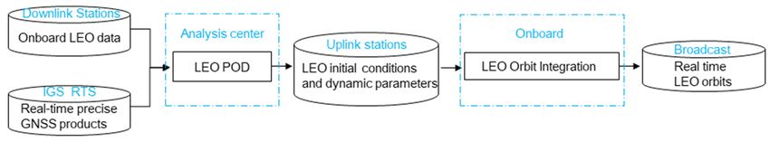
timeline of
uplinked
data process inistime and in
shown were delayed
Figure 2. Ifto betime
the uplinked
gap of atLEO
the next uplinkobservation
onboard station. Thedata timeline of datais shorter,
collection
process is shown in Figure 2. If the time
the length of orbit prediction time can be even shorter.gap of LEO onboard observation data collection is shorter,
the length of orbit prediction time can be even shorter.
Figure 2. Timeline of the data process.
Figure 2. Timeline of the data process.
With these procedures, we proposed three strategies to fulfill LEO prediction. We took GRACE-A
With these procedures, we proposed three strategies to fulfill LEO prediction. We took
data for example with its data from Day Of Year (DOY) 010, 2007 to DOY 360, 2007. As aforementioned,
GRACE-A data for example with its data from Day Of Year (DOY) 010, 2007 to DOY 360, 2007. As
theaforementioned,
LEO initial conditions and conditions
the LEO initial dynamic and parameters determinate
dynamic parameters the precision
determinate of predicted
the precision of LEO
orbits. TheLEO
predicted accelerometer measures all
orbits. The accelerometer non-gravitational
measures forces forces
all non-gravitational actingacting
on the
on satellite.
the satellite.However,
theHowever,
measurement has to be calibrated
the measurement in termsin
has to be calibrated ofterms
bias and scale
of bias andwhen
scale they
whenare
theyused to process
are used to orbit
process orbit determination. The bias and scale have to be estimated together with the
determination. The bias and scale have to be estimated together with the LEO initial position andLEO initial
positionThe
velocity. andcalibration
velocity. Themodel
calibration model
can be can be
written aswritten as
= + (1)
ang = B + Ka (1)
where denotes the non-gravitational acceleration. = B h B B denotes
iT the bias vector.
where ang denotes
= diag K K the
K non-gravitational
denotes the scale acceleration.
matrix. B = theBX
denotes BY BZ
non-gravitational denotes the bias vector.
measurement.
h i
K Note
= diagboth KX andKY Kare Z indenotes
the GRACE Science
the scale Reference
matrix. Frame
a denotes the(SRF), while LEO POD
non-gravitational is
measurement.
conducted in the inertial system. Thus, one needs to transform from SRF to the inertial
Note both ang and a are in the GRACE Science Reference Frame (SRF), while LEO POD is conducted in frame,
thewhich is system. Thus, one needs to transform a from SRF to the inertial frame, which is
inertial ng
= = +
(2)
aCIS = Mang = M(B + Ka) (2)
where is the transform matrix from SRF to the inertial frame.
where M is the transform matrix from SRF to the inertial frame.
The proposed three strategies are mainly focused on the determination of dynamic parameters
The POD
in LEO proposed three
and they arestrategies
as follows.are mainly focused on the determination of dynamic parameters in
LEO POD and they are as follows.
Strategy 1: Accelerometer data are used with the calibration parameters of biases and scale factors
in each axis for one arc, which are named as BX , BY , BZ , KX , KY , and KZ . For simplicity and easy
reading, ACC_B_K is used in the following study referring to this strategy.
Strategy 2: Accelerometer data are used with the calibration parameters of biases in each axis
every 60 min, which are named as BX , BY , and BZ and scale factors for three directions are equal to one.
This strategy is called ACC_B in the following.Remote Sens. 2020, 12, 1599 5 of 18
Strategy 3: Empirical force models are used with the dynamic coefficients of Ca, Sa, Cc, and Sc for
along- and cross-track directions (cosine/sine), and a scale factor for the atmospheric drag every one
cycle per revolution. EMP is used referring to this strategy in the following.
Strategy 1 (ACC_B_K) and 2 (ACC_B) are different at the estimation of calibration parameters of
the accelerometer, which are based on the GFZ GRACE Level-2 processing standards document [30,31].
Strategy 3 (EMP) was conducted to show the precision of predicted LEO orbits with empirical force
models. Actually, there is a shortcoming with the method using accelerometer data, for which
orbit prediction must be conducted onboard, since real time accelerometer data should be acquired.
The empirical method is simple that one can conduct the orbit prediction at the analysis center,
then uplink the LEO orbits to the corresponding LEO satellites.
The batch least square approach was used to estimate the LEO initial position and velocity as well
as dynamic parameters. The force models, observation models, and the parameters to be estimated in
LEO POD are listed in Table 1.
Table 1. Force models, observation models, and estimated parameters of LEO POD with
different strategies.
Force Models Description ACC_B_K ACC_B EMP
√ √ √
Earth gravity EIGEN-6C [32] 120 × 120
√ √ √
N-body JPL DE405 [33]
√ √ √
Solid earth tide IERS Conventions 2010 [34]
√ √ √
Ocean tide EOT11a [35]
√ √ √
Relativity effect IERS Conventions 2010 [32]
√
Atmosphere drag DTM94 [36] × ×
√
Solar radiation Macro model [37] × ×
√ √ √
Observation models
√ √ √
Observation Un-differenced ionosphere-free code and phase combination
√ √ √
Arc length 24 h
√ √ √
Sampling rate 30 s
√ √ √
Cutoff elevation 3◦
√ √ √
Phase wind up Applied [38]
√ √ √
LEO phase centre offset Applied [39]
√ √ √
GPS phase centre offset igs08.atx [40]
√ √ √
Relativity effect IERS Conventions 2010 [32]
Tropospheric delay Not relevant × × ×
Parameters
√ √ √
LEO orbits Initial conditions (positions and velocities)
√ √ √
Receiver clock Estimated as white noise
√
Atmosphere drag A scale factor estimated every one cycle per revolution (1.5 h) × ×
Ca, Sa, Cc, and Sc for along- and cross-track directions (cosine/sine) √
Empirical force × ×
every one cycle per revolution √
Accelerometer scale KX , KY , and KZ , one set for one arc × ×
√ √
Accelerometer bias BX , BY , BZ , one set for one arc for ACC_B_K, every 60 min for ACC_B ×
√ √ √
Phase ambiguity One per satellite per pass (float solution)
As recorded by the GRACE Science data system monthly report, the Disabling of Supplemental
Heater Lines (DSHL) of GRACE-A would cause temperature control on accelerometer to be stopped.
The cool down of the accelerometer caused the accelerometer biases to change and the reheating of the
accelerometer returned the accelerometer biases to near nominal values after some days, which would
affect POD by using accelerometer data. For this reason, these days are excluded in the following
analysis, such as the data from 17th to 21st January (DOY: 017 to 021, 2007) and from 22nd to 26th
November (DOY: 326 to 330, 2007). We used the slide window process to simulate the real time process.
The length of slide window is equal to the length of prediction time. So, we have 24 sets of results in
one day if the length of prediction time is one hour.
3. Analysis of Dynamic Parameters
In this section, we first checked the precision of LEO orbits by using precise GNSS products with
those three strategies. Here, we used CODE (Center for Orbit Determination in Europe) precise GPS
orbit and 30 s clock products since there was no real time precise orbit and clock products in 2007
(ftp://cddis.gsfc.nasa.gov/pub/gps/products, [41]). Furthermore, one has to collect and store real timeto 26th November (DOY: 326 to 330, 2007). We used the slide window process to simulate the real
time process. The length of slide window is equal to the length of prediction time. So, we have 24
sets of results in one day if the length of prediction time is one hour.
3. Analysis of Dynamic Parameters
Remote Sens. 2020, 12, 1599 6 of 18
In this section, we first checked the precision of LEO orbits by using precise GNSS products
with those three strategies. Here, we used CODE (Center for Orbit Determination in Europe) precise
orbit GPS orbit and
and clock 30 s clock
corrections byproducts sincesince
themselves thereno
was no real
public time is
archive precise orbitfor
available andthe
clock products
storage in
of previous
2007orbit
real time (ftp://cddis.gsfc.nasa.gov/pub/gps/products,
and clock products. More details about [41]).
the Furthermore,
impact on LEO onePOD
has to
withcollect
real and
timestore
products
real time
and final orbit and
products canclock corrections
be found byAppendix
in the themselvesA. since
The noPrecise
public archive
Scienceis Orbits
available for the
(PSO) ofstorage
GRACE-A
of previous real time orbit and clock products. More details about the impact on LEO POD with real
provided by Jet Propulsion Laboratory (JPL) was used as references for our orbit evaluation in this
time products and final products can be found in the Appendix. The Precise Science Orbits (PSO) of
article (https://podaac-tools.jpl.nasa.gov/drive/files/allData/grace/L1B/JPL). Then the accelerometer
GRACE-A provided by Jet Propulsion Laboratory (JPL) was used as references for our orbit
calibration parameters
evaluation as well
in this article as the parameters of empirical models were also investigated
(https://podaac-tools.jpl.nasa.gov/drive/files/allData/grace/L1B/JPL). Thenfor the
first two strategies. Figure 3 shows the averaged Root Mean Square (RMS) values
the accelerometer calibration parameters as well as the parameters of empirical models were also for along-track,
cross-track, and radial
investigated for thedirections with the three
first two strategies. Figurestrategies,
3 shows therespectively. The corresponding
averaged Root Mean Square (RMS) averaged
RMS values
valuesforof along-track,
all days forcross-track,
three directions are shown
and radial in Table
directions 2. three strategies, respectively. The
with the
corresponding averaged RMS values of all days for three directions are shown in Table 2.
Figure 3. Averaged
Figure Root Mean
3. Averaged Square
Root Mean (RMS)(RMS)
Square valuesvalues
for along-track, cross-track,
for along-track, and radial
cross-track, directions
and radial
with directions
the three strategies.
with the three strategies.
Averaged
Table 2.the
In general, RMSare
RMS values values on allfor
smallest days for three directions
all directions with three
when empirical strategies.
force models are used.
These empirical models can efficiently absorb the unmodeled part of the non-gravitational forces.
Along-Track (mm) Cross-Track (mm) Radial (mm)
The averaged RMS values for all days were 12.1 mm, 6.2 mm, and 6.8 mm for along-track,
ACC_B_K
cross-track, and 23.3
radial direction, respectively. 14.3
For radial direction, 6.8
the RMS values of the two
ACC_B 11.8 11.9 6.1
EMP 12.1 6.2 6.8
In general, the RMS values are smallest for all directions when empirical force models are used.
These empirical models can efficiently absorb the unmodeled part of the non-gravitational forces.
The averaged RMS values for all days were 12.1 mm, 6.2 mm, and 6.8 mm for along-track, cross-track,
and radial direction, respectively. For radial direction, the RMS values of the two strategies using
accelerometer data were nearly the same as using the empirical force models with about 6.8 mm,
while the RMS values of cross-track direction were larger than that of empirical method, which were
14.3 mm and 11.9 mm for the ACC_B_K method and ACC_B method. This is mainly caused by the
sensitivity of the accelerometer [42]. The more sensitive axes point in the flight and radial directions,
the less sensitive axis points in the cross-track direction [26]. The precision of the sensitive axes is
specified to be 10−10 m/s2 and that of the less sensitive axis 10−9 m/s2 [27]. The RMS values of the
along-track direction for the strategy of estimating the accelerometer bias every one hour and empirical
forces were almost the same at about 12.0 mm while the strategy of estimating the accelerometer bias
and scale for one day were worse than those two strategies with 23.3 mm. Such a difference may be
caused by the number of estimated parameters. The number of estimated dynamic parameters of the
three strategies is 6 (BX , BY , BZ , KX , KY , and KZ ), 72 (BX , BY , and BZ every one hour for 24 h, 24 × 3 = 72),
and 80 (Ca, Sa, Cc, Sc, and a scale factor every one cycle per revolution for 24 h, 24/1.5 × 5 = 80),dynamic parameters of the three strategies is 6 (BX, BY, BZ, KX, KY, and KZ), 72 (BX, BY, and BZ every
one hour for 24 hours, 24 × 3 = 72), and 80 (Ca, Sa, Cc, Sc, and a scale factor every one cycle per
revolution for 24 hours, 24/1.5 × 5 = 80), respectively. In the least square estimator, the more
parameters, the smaller the fitted residuals if all parameters are estimable.
Remote Sens. 2020, 12,Table
1599 2. Averaged RMS values on all days for three directions with three strategies. 7 of 18
Along-track (mm) Cross-track (mm) Radial (mm)
ACC_B_K
respectively. In the least square estimator, 23.3 the more parameters,
14.3 the smaller6.8 the fitted residuals if all
parameters are estimable. ACC_B 11.8 11.9 6.1
EMP 12.1 6.2 6.8
The initial conditions and dynamic parameters estimated from the POD process are then used
The initial conditions and dynamic parameters estimated from the POD process are then used
for the LEO orbit prediction. It is of great importance to analyze dynamic parameters since they will
for the LEO orbit prediction. It is of great importance to analyze dynamic parameters since they will
have a direct effect on the orbit precision for orbit prediction. If only one set dynamic parameters
have a direct effect on the orbit precision for orbit prediction. If only one set dynamic parameters is
is estimated
estimated forforone
onearc,
arc,then
thenthese
these estimated parameters
estimated parameters areare used
used forfor
LEOLEO orbit
orbit prediction,
prediction, such such
as as
strategy 1 (ACC_B_K). If there are more than one set of dynamic parameters estimated
strategy 1 (ACC_B_K). If there are more than one set of dynamic parameters estimated like strategy like strategy 2
(ACC_B) and 3 and
2 (ACC_B) (EMP), one has
3 (EMP), oneto firstly
has investigate
to firstly thethe
investigate characteristics
characteristicsofofthe
thedynamic
dynamic parameters
parameters and
then and
decide
thenthe waythe
decide to way
predict the LEO
to predict the orbit. Figure
LEO orbit. 4 shows
Figure 4 showsthetheaccelerometer
accelerometer bias parameters for
bias parameters
for strategy
strategy 2. 2.
Figure 4. Accelerometer
Figure 4. Accelerometer bias
biasparameters
parameters for
for strategy 2. The
strategy 2. Thedata
data between
between black
black dashed
dashed lineslines
are are
excluded because of the change of the controller onboard or abnormal behavior
excluded because of the change of the controller onboard or abnormal behavior of accelerometer. of accelerometer.
BlackBlack
lineslines
are the linear
are the fitting
linear line.
fitting line.The
Thecorresponding fittingresults
corresponding fitting resultsare
are also
also shown
shown in each
in each panel.
panel.
The behavior of three
The behavior biases
of three waswas
biases different forfor
different thethe
three
threedirections.
directions.By
Bylinear
linear fitting,
fitting, we could
could find
that biases in the
find that y direction
biases in the y show a clear
direction showsmooth
a cleartrend
smoothin the year.
trend It changed
in the about 10,450
year. It changed aboutnm/s 2 in the
10,450
year. nm/s
For the x direction, there was also a small trend, which was about -9 nm/s2 in-92007.
2 in the year. For the x direction, there was also a small trend, which was about nm/s2Biases
in 2007.
in the
2
z direction keep quite stable, which was only 1.3 nm/s in the year. Due to this increased or decreased
trend of the biases, it may not be appropriate using the last set of accelerometer calibration parameters
to conduct the real time orbit prediction and linear fitting and an extrapolation should be used when
doing the orbit integration for real time LEO orbits. Figure 5 shows the averaged RMS of calibration
parameters’ differences between using the extrapolated calibration parameters for one hour and the
estimated ones as well as the averaged RMS of calibration parameters’ differences between using the
last set of calibration parameters and estimated ones for each arc.
From Figure 5, we can see that the extrapolated calibration parameters are much closer to the
estimated ones, which means the precision of the predicted orbit by using extrapolated calibration
parameters should be higher than that of using the last set of calibration parameters. The accelerometer
bias in the y direction shows the largest difference since this direction is the least sensitive for the
accelerometer instrument, which is pointing to the cross-track direction of the LEO orbit while the bias
in the x direction shows the smallest difference. In the following LEO orbit prediction analysis, we will
use the extrapolation calibration parameters for orbit prediction with strategy 2.
Figure 6 shows the dynamic parameters in the EMP method. It shows that the dynamic parameters
are not stable, especially for the Sa and Ca terms, which are used for compensating the unmodeled
part of the along-track component. They are quite different from day to day. This also implies that the
non-gravitational force models used in the POD are not accurate enough and the dynamic parameters
have to be estimated in order to absorb the unmodeled part of non-gravitation. It is not appropriate toRemote Sens. 2018, 10, x FOR PEER REVIEW 8 of 19
Biases in the z direction keep quite stable, which was only 1.3 nm/s2 in the year. Due to this
increased or decreased trend of the biases, it may not be appropriate using the last set of
accelerometer calibration parameters to conduct the real time orbit prediction and linear fitting and
Remote Sens. 2020, 12, 1599 8 of 18
an extrapolation should be used when doing the orbit integration for real time LEO orbits. Figure 5
shows the averaged RMS of calibration parameters’ differences between using the extrapolated
use calibration
the extrapolateparameters
methodfor one hour
to obtain and the
dynamic estimatedfor
parameters ones
orbitasprediction
well as the
likeaveraged RMS
the ACC_B of
method
calibration
since parameters’
these parameters differences
fluctuated between
and are hard tousing the So,
predict. lastthe
setlast
of set
calibration
of dynamicparameters andwas
parameters
estimated
adopted ones for
to predict theeach arc.
orbit in the following parts for the EMP method.
Figure 5. Averaged RMS of calibration parameters’ differences between using the extrapolated
Figure 5. Averaged RMS of calibration parameters’ differences between using the extrapolated
calibration parameters and the estimated ones as well as the averaged RMS of calibration parameters’
calibration parameters and the estimated ones as well as the averaged RMS of calibration
differences between using the last set of calibration parameters and the estimated ones for each arc.
parameters’ differences between using the last set of calibration parameters and the estimated ones
Remote Sens. 2018, 10, x FOR PEER REVIEW 9 of 19
“W/O Extro” means
for each arc. “W/O without extrapolated
Extro” means withoutand “W Extro”
extrapolated means
and with extrapolation.
“W Extro” means with extrapolation.
From Figure 5, we can see that the extrapolated calibration parameters are much closer to the
estimated ones, which means the precision of the predicted orbit by using extrapolated calibration
parameters should be higher than that of using the last set of calibration parameters. The
accelerometer bias in the y direction shows the largest difference since this direction is the least
sensitive for the accelerometer instrument, which is pointing to the cross-track direction of the LEO
orbit while the bias in the x direction shows the smallest difference. In the following LEO orbit
prediction analysis, we will use the extrapolation calibration parameters for orbit prediction with
strategy 2.
Figure 6 shows the dynamic parameters in the EMP method. It shows that the dynamic
parameters are not stable, especially for the Sa and Ca terms, which are used for compensating the
unmodeled part of the along-track component. They are quite different from day to day. This also
implies that the non-gravitational force models used in the POD are not accurate enough and the
dynamic parameters have to be estimated in order to absorb the unmodeled part of non-gravitation.
It is not appropriate to use the extrapolate method to obtain dynamic parameters for orbit
prediction like the ACC_B method since these parameters fluctuated and are hard to predict. So, the
last set of dynamic parameters was adopted to predict the orbit in the following parts for the EMP
method.
Figure 6. Dynamic parameters estimated from Strategy 3.
Figure 6. Dynamic parameters estimated from Strategy 3.
4. Results of LEO Orbit Prediction
After conducting LEO POD, the initial conditions as well as the dynamic parameters can be
uplinked to the corresponding LEO satellites. Then the processor on LEO satellites can do orbit
prediction/propagation for real time applications. We used one hour for orbit prediction as
mentioned before. One issue should be clarified here. If we used the EMP method in which empiricalRemote Sens. 2020, 12, 1599 9 of 18
4. Results of LEO Orbit Prediction
After conducting LEO POD, the initial conditions as well as the dynamic parameters can be
uplinked to the corresponding LEO satellites. Then the processor on LEO satellites can do orbit
prediction/propagation for real time applications. We used one hour for orbit prediction as mentioned
before. One issue should be clarified here. If we used the EMP method in which empirical force models
are applied, the orbit prediction could also be conducted at the analysis center in advance since no real
time onboard observations are required whereas for the ACC_B_K and ACC_B method, it must be
conducted onboard because real time accelerometer data must be used.
The initial conditions and the dynamic parameters have great impact on the precision of LEO orbit.
For the EMP method, the last set of empirical coefficients were chosen for real time orbit integration
as usual and for the ACC_B_K method there was only one set of calibrations parameters for each
direction including scales and biases for the orbit integration. For the ACC_B method, we used a
linear fitting for the previous 24-h arc since an obvious trend could be found in these biases, and then
extrapolated the biases according to the integration time.
The differences between PSO and predicted orbits were calculated for the orbit evaluation and
their User Ranging Error (URE) were also calculated and compared. URE provides the average range
error in the line-of-sight direction at a global scale. Its computation is related to the maximum satellite
coverage on the Earth’s surface. The coverage depends on the angular range of the satellite, which is
the angle of the emission cone with respect to the boresight direction. With the angular range of LEO
satellites at the altitude of 500 km being about 68.02◦ , the URE can be approximately determined
as [8,9,43]: q
Remote Sens. 2018, 10, x FOR PEER REVIEW 10 of 19
URE = 0.205(RMSR )2 + 0.397 (RMSA )2 + (RMSC )2
(3)
Figure
Figure 7 shows
7 shows thethe averaged
averaged RMSRMS values
values ofof a one
a one hour
hour predictedorbit
predicted orbitininthree
threedirections
directionswith
withthe
the three strategies. The corresponding averaged RMS values of all days for each direction
three strategies. The corresponding averaged RMS values of all days for each direction with different with
differentare
strategies strategies
shown are shown
at the at the
top left of top
eachleft of each panel.
panel.
Figure 7. Averaged RMS values for the three directions with three strategies for an orbit prediction of
Figure 7. Averaged RMS values for the three directions with three strategies for an orbit prediction of
one hour.
one hour.
It is easy to find out that the ACC_B_K strategy shows the best results, especially for along-track
It is easy to find out that the ACC_B_K strategy shows the best results, especially for
direction at 4.8 cm while the ACC_B and EMP strategies were at 15.6 cm and 31.5 cm. For the radial
along-track direction at 4.8 cm while the ACC_B and EMP strategies were at 15.6 cm and 31.5 cm.
direction, the RMS values were 1.7 cm, 3.7 cm, and 8.6 cm for the ACC_B_K, ACC_B, and EMP strategy,
For the radial direction, the RMS values were 1.7 cm, 3.7 cm, and 8.6 cm for the ACC_B_K, ACC_B,
respectively. The RMS value of cross-track direction for the ACC_B_K strategy was 4.3 cm, which was
and EMP strategy, respectively. The RMS value of cross-track direction for the ACC_B_K strategy
was 4.3 cm, which was worse than the other two strategies with 1.6 cm and 1.7 cm. As Figure 8
shows, the averaged URE values for the three strategies were 4.4 cm, 10.1 cm, and 20.3 cm,
respectively.one hour.
It is easy to find out that the ACC_B_K strategy shows the best results, especially for
along-track direction at 4.8 cm while the ACC_B and EMP strategies were at 15.6 cm and 31.5 cm.
For the radial direction, the RMS values were 1.7 cm, 3.7 cm, and 8.6 cm for the ACC_B_K, ACC_B,
Remote Sens. 2020, 12, 1599 10 of 18
and EMP strategy, respectively. The RMS value of cross-track direction for the ACC_B_K strategy
was 4.3 cm, which was worse than the other two strategies with 1.6 cm and 1.7 cm. As Figure 8
shows,
worse thanthetheaveraged
other twoURE values with
strategies for the
1.6 three
cm andstrategies
1.7 cm. were 4.4 cm,
As Figure 10.1 cm,
8 shows, the and 20.3 cm,
averaged URE
respectively.
values for the three strategies were 4.4 cm, 10.1 cm, and 20.3 cm, respectively.
Figure 8. User Ranging Error (URE) of a real time LEO orbit for three different strategies.
Figure 8. User Ranging Error (URE) of a real time LEO orbit for three different strategies.
It is easy to understand that predicted LEO orbit precision by using accelerometer data were
better than that of using empirical force models since accelerometer data could better reflect the
non-gravitational forces than that of the empirical force models. We found that with the method of
strategy 1 (ACC_B_K), the predicted LEO orbit precision shows a better result in the along and radial
directions than with strategy 2 (ACC_B), though the calculation part (orbit determination part) of
ACC_B_K of the along-track and radial directions was worse than those of ACC_B. We calculated the
differences of the predicted non-gravitational acceleration between ACC_B_K and the corresponding
non-gravitational acceleration calculated from estimated biases and the scale factor as well as
the differences of predicted non-gravitational acceleration between ACC_B and the corresponding
non-gravitational acceleration calculated from estimated biases for a one hour prediction, as shown in
Figure 9.
From Figure 9, we can see that the difference of non-gravitational accelerations in the x direction
(orbit along-track direction) and z direction (radial direction) with the ACC_B_K method were much
smaller than those of the ACC_B method, which means that the along-track and radial direction
precision of the prediction part with ACC_B_K should be better than those of the ACC_B method.
For the cross-track direction (y direction of acceleration), the differences between the predicted
acceleration and the calculated one with the ACC_B_K method were larger than that of the ACC_B
method, which corroborated the worse results of the cross-track direction with the ACC_B_K method.
In conclusion, one set of scales and biases for each direction reflected the calibration parameters
of the accelerometer for the long term while one set of biases every hour reflected for the short term.
For orbit prediction for less than 20 min, the precision of all orbit components with all strategies was
better than 10 cm. This means that if the interval of the uplink and downlink was shorter than 20 min,
all strategies could be used for real time LEO POD. For orbit prediction for more than 20 min, the best
way to realize the real time LEO precise orbit determination is by using accelerometer data with the
estimation of one set of scales and biases for each direction. In this way, less than a 5 centimeter level of
LEO orbit precision can be achieved for the one hour LEO orbit prediction, which satisfies the demand
of a centimeter level requirement mentioned in the Introduction section.were much smaller than those of the ACC_B method, which means that the along-track and radial
direction precision of the prediction part with ACC_B_K should be better than those of the ACC_B
method. For the cross-track direction (y direction of acceleration), the differences between the
predicted acceleration and the calculated one with the ACC_B_K method were larger than that of the
ACC_B method, which corroborated the worse results of the cross-track direction with the
Remote Sens. 2020, 12, 1599 11 of 18
ACC_B_K method.
Figure 9. Differences of predicted non-gravitational acceleration between the ACC_B_K method and
Figure
the 9. Differences
calculated ones as of predicted
well non-gravitational
as the differences acceleration
of predicted between the
non-gravitational ACC_B_K between
acceleration method and
the
the calculated ones as well as the differences of predicted non-gravitational acceleration
ACC_B method and the calculated ones for a one hour prediction in each direction. “Oneday dif” between the
ACC_B
means
Remote method
Sens.the ACC_B_K
2018, and the calculated
10, x FOR method ones for a one hour prediction
and “Onehour dif” means the ACC_B method.
PEER REVIEW in each direction. “Oneday dif”
12 of 19
means the ACC_B_K method and “Onehour dif” means the ACC_B method.
Usually,
Usually,most
most precise
precisepositioning
positioning users
userscare more
care more about
about the
theorbit
orbiterrors forforevery
errors everyepoch
epochwhile
whilenot
fornotInfor
the conclusion,
the averaged
averaged onesone set
ones
over of over
one scales
hour. and
one biases
hour.
Figure for each
10Figure
shows 10RMSdirection
shows RMS
values reflected
of values the calibration
of LEO
LEO orbits parameters
orbitsdirections
for three for three of
of directions
the 10
every accelerometer
minof every
over for
a one10the long
minutes
hour term
overwhile
prediction oneone
a time set prediction
hour
period.of The
biases every
greattime hour reflected
period.
increase The greatfor the
of along-track shortvalues
increase
RMS term.
of
For orbit prediction
along-track RMS for
values less
withthanthe20 minutes,
empirical the
methodprecision
can be of all
easily orbit
found, components
which
with the empirical method can be easily found, which is from about 5.0 cm at 10 min to approximately is fromwith all
about strategies
5.0 cm
wasatcm
49.4 10 over
minutes
better than
one10to approximately
cm.
hour. This means
However, 49.4
thethat cm over
if the
method oneaccelerometer
interval
with hour. However,
of the uplink
data the
and method
downlink
with one set with
was accelerometer
shorter
of biases andthan 20
scales
fordata
eachwith
minutes, allone setshows
of biases
strategies
direction could andbe scales
a stable RMSfor
used ofeach
real direction
time4.0
4.9 cm, LEO shows
cm, anda1.2
POD. stable
For RMS
orbit
cm ofalong-track,
4.9 cm, for
prediction
in the 4.0 cm,
more and 1.2 20
than
cross-track,
andcm in the
minutes,
radial along-track,
the best way
directions all cross-track,
to time,
the realize and
theradial
real directions
respectively. time LEO all precise
the time,orbit
respectively.
determination is by using
accelerometer data with the estimation of one set of scales and biases for each direction. In this way,
less than a 5 centimeter level of LEO orbit precision can be achieved for the one hour LEO orbit
prediction, which satisfies the demand of a centimeter level requirement mentioned in the
Introduction section.
Figure 10. RMS values of LEO orbits for the along-track, cross-track, and radial direction for every 10
Figure 10. RMS values of LEO orbits for the along-track, cross-track, and radial direction for every 10
min over a over
minutes one hour
a oneperiod.
hour period.
The corresponding URE for every 10 min is shown in Figure 11. The method with accelerometer
The corresponding URE for every 10 minutes is shown in Figure 11. The method with
data with one set of biases and scales for each direction shows the most stable results about 4.6 cm
accelerometer data with one set of biases and scales for each direction shows the most stable results
even if the
about 4.6integration
cm even time
if theis integration
one hour while
timethe
is method
one hourof while
empirical
the and accelerometer
method dataand
of empirical with
accelerometer data with one-hour biases for each direction shows an increased trend, from about 4.6
cm at 0-10 minutes to 31.4 cm and 14.0 cm within 50-60 minutes.Figure 10. RMS values of LEO orbits for the along-track, cross-track, and radial direction for every 10
minutes over a one hour period.
The corresponding URE for every 10 minutes is shown in Figure 11. The method with
Remote Sens. 2020, 12,data
accelerometer 1599 with one set of biases and scales for each direction shows the most stable results
12 of 18
about 4.6 cm even if the integration time is one hour while the method of empirical and
accelerometer data with one-hour biases for each direction shows an increased trend, from about 4.6
one-hour biases for each direction shows an increased trend, from about 4.6 cm at 0-10 min to 31.4 cm
cm at 0-10 minutes to 31.4 cm and 14.0 cm within 50-60 minutes.
and 14.0 cm within 50-60 min.
Figure 11. URE for every 10 min over a one hour orbit prediction.
Figure 11. URE for every 10 minutes over a one hour orbit prediction.
As mentioned above in the “LEO orbit prediction procedure”, if the orbital elements do not uplink
in time, one has to wait until the next uplink, which means a delay of nearly two hours. The RMS
Remote
values ofSens.
LEO 2018, 10, x for
orbits FORthree
PEER REVIEW 13 of URE
directions with another one hour prediction and the corresponding 19
values are shown in Figure 12.
As mentioned above in the “LEO orbit prediction procedure”, if the orbital elements do not
We could easily find that the method with accelerometer data with one set of biases and scales for
uplink in time, one has to wait until the next uplink, which means a delay of nearly two hours. The
each direction (ACC_B_K) still shows the most stable results while the method with empirical models
RMS values of LEO orbits for three directions with another one hour prediction and the
(EMP) fluctuated, especially in the radial component. The RMS value for the along-track component
corresponding URE values are shown in Figure 12.
could be at one meter for the method with empirical models while it is still better than 10 cm for the
method with one set of biases and scales.
Figure 12. Cont.Remote Sens. 2020, 12, 1599 13 of 18
Figure 12. RMS values of LEO orbits for the along-track, cross-track, and radial direction for another
Figure 12. RMS values of LEO orbits for the along-track, cross-track, and radial direction for another
oneone
hour and
hour andcorresponding URE
corresponding UREvalues.
values.
5. Conclusions
We could easily find that the method with accelerometer data with one set of biases and scales
forWith
eachthe development
direction of thestill
(ACC_B_K) LEOshows
related
themissions and results
most stable applications,
while there will bewith
the method a great demand
empirical
models
of real time(EMP)
LEO fluctuated, especially
precise orbit. In this in the radial
study, three component. The estimation
strategies with RMS value of fordifferent
the along-track
dynamic
component
parameters could
were be at oneand
conducted meter
thefor the methodare
conclusions with empirical models
summarized while it is still better than 10
as follows
cm for the method with one set of biases and scales.
(1) The precision of LEO satellites orbits could reach the centimeter level with estimation of different
5. Conclusions
kinds of dynamic parameters if precise GNSS products were adopted. However, under the
current circumstances, RTS was not available for onboard processing. For the demand of the real
time precise LEO orbit, at least a one-hour orbit prediction should be adopted.
(2) For the current GNSS technology, LEO orbit prediction by using accelerometer data was feasible.
Precision of one hour predicted LEO satellite orbits with initial conditions and dynamic parameters
estimated with a 24 h arc could reach the centimeter level by using accelerometer data while that
using empirical force models was at the decimeter level.
(3) For the LEO orbit prediction over 20 min, the predicted LEO orbit precision with estimation of
one set of biases and scales for each direction (strategy 1) was better than that of biases for each
direction every 60 min (strategy 2), though the calculated orbit precision with the latter was better
than the former method.
(4) If there were enough uplink and downlink stations, which mean the interval of uplink and
downlink could be shorter than 20 min, all these three strategies could be adopted for the real
time applications.
On all accounts, the accelerometer data had great potential to do the LEO orbit prediction for real
time applications in the near future.
6. Discussions
This article aimed at investigating centimeter level precision of LEO orbit prediction for real
time applications. It is a good replacement of using accelerometer data instead of empirical force
models when conducting LEO orbit prediction. Three strategies with estimation of different dynamic
parameters were conducted. The results show that with our proposed method, the LEO orbit precision
could reach the centimeter level and even predicting within two hours. Two more practical issues
should be clarified.Remote Sens. 2020, 12, 1599 14 of 18
The first one is the feasibility of widespread use of accelerometers. The idea of using accelerometers
for orbit prediction is a good idea and it was already shown in this study. However, the accelerometers
we used were of high quality for specific missions, such as a gravity mission. Such accelerometers
may be too expensive for the mass market. Concerning this issue, experiments (one can add colored
or white noise in the accelerometer data) could be conducted in the future to check the tolerance of
accelerometer data with respect to the precision of orbit prediction.
The second issue is the time gap of LEO onboard observation data collection. We took GRACE-A
as example, which has an inclination of 89◦ . It is quite easy to have a continuous coverage for sustained
period (half cycle of the LEO orbital period) where the uplink and downlink station are located at
high latitudes (north and south). However, more uplink and downlink stations are needed of LEO
satellites with low orbital inclination to meet the max length of the LEO orbit prediction (such as about
20 min for GRACE-A to keep the centimeter precision of the orbit prediction with empirical models).
The distribution of the uplink and downlink stations for different inclinations of LEO satellites should
be investigated to guarantee the time gap of onboard data collection.
Author Contributions: All authors contributed to the writing of this manuscript. H.G., B.L., and M.G. conceived
the idea of employing accelerometer data to conduct LEO orbit prediction. H.G. and L.N. processed the data
and investigated the results. M.G., B.L., and H.S. validated the data. All authors have read and agreed to the
published version of the manuscript.
Funding: This study is sponsored by National Natural Science Foundation of China (41874030), The Scientific
and Technological Innovation Plan from Shanghai Science and Technology Committee (18511101801), and The
National Key Research and Development Program of China (2017YFA0603102), and the Fundamental Research
Funds for the Central Universities.
Acknowledgments: Thanks to Physical Oceanography Distributed Active Archive Center (PO. DAAC) of JPL for
providing the raw GNSS observations and post-processed reduced dynamic orbit of GRACE-A and GRACE-C.
The GNSS observations and orbit products are available from https://podaac-tools.jpl.nasa.gov/drive/files/allData/
grace/L1B/JPL and https://podaac-tools.jpl.nasa.gov/drive/files/allData/gracefo/L1B/JPL/RL04/ASCII for GRACE-A
and GRACE-C, respectively. We are also grateful to CODE and GFZ real time group for providing precise GPS
final products and real time products, respectively.
Conflicts of Interest: The authors declare no conflict of interest.
Abbreviations and Acronyms
The following acronyms and abbreviations are used in this manuscript:
CHAMP Challenging Minisatellite Payload
CODE Center for Orbit Determination in Europe
DOY Day of Year
DSHL Disabling of Supplemental Heater Lines
ESA European Space Agency
GFZ GeoForschungsZentrum
GNSS Global Navigation Satellite System
GOCE Gravity field and steady-state Ocean Circulation Explorer
GPS Global Positioning System
GRACE Gravity Recovery and Climate Experiment
GRACE-FO Gravity Recovery and Climate Experiment Follow-On
IGS International GNSS Service
JPL Jet Propulsion Laboratory
LEO Low Earth Orbit
LeGNSS Leo enhanced Global Navigation Satellite System
NRT Near Real Time
NTC Non Time Critical
POD Precise Orbit Determination
PPP Precise Point Positioning
RMS Root Mean Square
RTPP Real Time Pilot ProjectYou can also read