Leveraging Crowdsourced GPS Data for Road Extraction from Aerial Imagery
←
→
Page content transcription
If your browser does not render page correctly, please read the page content below
Leveraging Crowdsourced GPS Data for Road Extraction from Aerial Imagery
Tao Sun, Zonglin Di, Pengyu Che, Chun Liu, Yin Wang
Tongji University, Shanghai, China
{suntao, dizonglin, chepengyu, liuchun, yinw}@tongji.edu.cn
arXiv:1905.01447v1 [cs.CV] 4 May 2019
Abstract
Deep learning is revolutionizing the mapping indus-
try. Under lightweight human curation, computer has
generated almost half of the roads in Thailand on Open-
StreetMap (OSM) using high resolution aerial imagery.
Bing maps are displaying 125 million computer generated
building polygons in the U.S. While tremendously more ef-
ficient than manual mapping, one cannot map out every-
thing from the air. Especially for roads, a small prediction
gap by image occlusion renders the entire road useless for (a) Occlusions by trees, buildings, and shadows are challenging without GPS
routing. Misconnections can be more dangerous. Therefore
computer based mapping often requires local verifications,
which is still labor intensive. In this paper, we propose
to leverage crowd sourced GPS data to improve and sup-
port road extraction from aerial imagery. Through novel
data augmentation, GPS rendering, and 1D transpose con-
volution techniques, we show almost 5% improvements over
previous competition winning models, and much better ro-
bustness when predicting new areas without any new train-
ing data or domain adaptation.
(b) Roads susceptible to over connection in post-processing without GPS
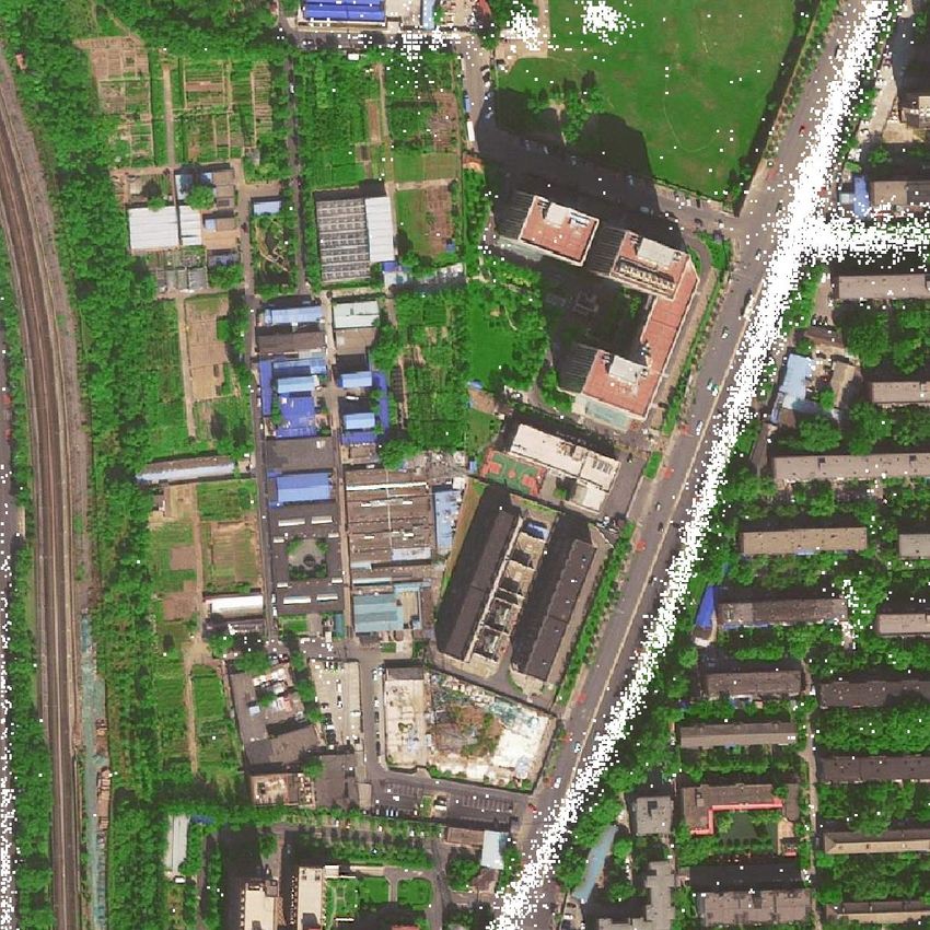
1. Introduction Figure 1: Crowdsourced GPS data helps road extraction
when aerial imagery alone is insufficient or challenging.
Segmentation of aerial imagery has been an active re- Here each red dot represents a taxi GPS sample.
search area for more than two decades [4, 17]. It is also
one of the earliest applications of deep convolutional neural
nets (CNN) [19]. Today, using deep convolutional neural features are indistinguishable from the air, e.g., dirt roads
nets over high resolution satellite imagery, Facebook has and bare fields, cement pavements and building tops, alleys
added 370 thousand km of computer generated roads to in slum areas. Bad weather, low satellite angle, and low
OpenStreetMap (OSM) [3] Thailand, accounting for 46 % light angle further complicate the issue. Even if the feature
of the total roads in the country, which is on display for all is perfectly clear, mapping often needs local knowledge.
Facebook users [1, 22]. Microsoft used similar techniques Trails and roads may have same appearances. Houses and
to add 125 million building polygons to Bing maps U.S., storage sheds may have similar sizes and roofs. To make
five times more than those on OSM [29]. things worse, mapping has low tolerance for errors. Espe-
Despite real-world applications, mapping by aerial im- cially for roads, incorrect routes cause longer travel time,
agery has its limitations. The top challenge is overfitting. lead people to restricted areas, and even cause fatal acci-
The deep neural net models often deteriorate miserably with dents [34]. Because of these reasons, OSM prefers local
new terrain, new building styles, new image styles, or new mappers for each area, and even requires local verification
resolutions. Other than the model limitation, occlusions by for large-scale edits [1].
vegetation, buildings, and shadows can be excessive. Many With a smart phone or any other GPS device, one
1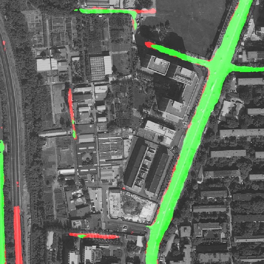
can easily travel a street and verify its existence with the           Semantic segmentation models based on the fully convolu-
recorded trace. Going through all streets systematically               tional neural net architecture become main stream [27]. In
and regularly for updates, however, is a labor intensive job           a recent challenge [10], all top solutions used variants of U-
that is costly and error prone. On the other hand, crowd-              net [24] or Deeplab [8] to segment an entire image at once,
sourced GPS data are much cheaper and increasingly abun-               up to 1024 x 1024 pixels. A larger input size gives more
dant [6, 12, 15, 26, 34]. Figure 1 illustrates how crowd-              context, which often leads to more structured and accurate
sourced GPS data, albeit noisy, can help discover roads,               prediction results.
confirm road continuity, and avoid misconnection.                          With new models and multi-country scale datasets, many
    In this paper, we propose to fuse crowdsourced GPS data            real-world applications emerge. Most notably, Facebook
with aerial imagery for road extraction. Through large taxi            has recently added 370 thousand km of roads extracted from
and bus GPS datasets from Beijing and Shanghai, we show                satellite imagery to OSM [3] Thailand, or 46 % of the to-
that crowdsourced GPS data has excessive noise in both                 tal roads in the country [1, 22]. Microsoft is displaying 125
variation and bias, and high degrees of disparity in density,          million computer generated building polygons on Bing US
resolution, and distribution. By rendering the GPS data as             maps, in contrast to the 23 million polygons from OSM
new input layers along with RGB channels in the segmen-                also on display that are mostly manually created or im-
tation network, together with our novel GPS data augmen-               ported [29].
tation techniques and 1D transpose convolution, our model                  Comparing to other computer vision applications, road
significantly outperforms existing models using images or              mapping has little margin for error. Prediction gaps make
GPS data alone. Our data augmentation is especially effec-             the entire road useless for routing, and therefore have at-
tive against overfitting. When predicting a new area, the              tracted lots of attention. Mnih noticed the problem early on
performance drop is much less than the model with image                and used Conditional Random Fields in post-processing to
input only, despite completely different GPS data quantity             link broken roads [18]. Another popular technique to link
and resolution. We will publish the code1 and our data is              roads is shortest path search [16, 33]. Line Integral Con-
available upon request.                                                volution can smooth out broken roads in post-processing
                                                                       too [14]. More recent works try to address the problem
2. Related Work                                                        in prediction instead of post-processing, e.g., through a
                                                                       topology-aware loss function [20] or through an iterative
    Aerial imagery segmentation has been a very active re-             search process guided by CNNs [5]. We must be careful
search area for a long time. We refer readers to some                  to link roads because incorrect connections are more dan-
performance studies and references therein for early algo-             gerous than missing connections in routing. Our approach
rithms [4,17]. Like many other image processing problems,              complements the above mentioned methods because GPS
these early solutions are often limited in accuracy and diffi-         data can confirm the connectivity or the absence of it re-
cult to generalize to real-world datasets.                             gardless of image occlusion or other issues.
    Mnih first used a deep convolutional neural net similar to             Road inferencing from GPS traces has been studied for
LeNet [13] to extract roads and buildings from a 1.2 m/pixel           a long time too [9, 23, 25]. Most early works use dense
dataset in the U.S. [18, 19]. Moving to developing coun-               GPS samples from controlled experiments. Recent works
tries with more diversified roads and buildings, Facebook              explored crowdsourced GPS data under various sampling
showed that deeper neural nets perform much better on a                interval and noise levels [6, 12, 15, 26, 34]. Kernel Density
50 cm/pixel dataset [33]. Both of these early approaches               Estimation is a popular method robust against GPS noise
convert the semantic segmentation problem into a classifi-             and disparity [6, 9, 15].
cation problem by classifying each pixel of a center square,               There is limited research work using both GPS data and
e.g., 32 x 32, as road or building from a larger image patch,          aerial imagery. One idea filters out GPS noise by road seg-
e.g., 128 x 128. Stitching these center squares together is            mentation before road inferencing [37]. Our preliminary
the final output for a large input image. Performance issues           work explored the idea of rendering GPS data as a new
aside, this classification approach cannot learn complicated           CNN input layer, but the segmentation model used was a
structures such as street blocks and building blocks due to            bit outdated and the GPS data was from a controlled exper-
limited input size.                                                    iment [28]. This paper experiments with many state-of-the-
    With the commercial availability of 30 cm/pixel satel-             art segmentation models and crowdsourced GPS datasets
lite imagery and low-cost aerial photography drones, more              several orders of magnitude bigger and noisier.
public high-resolution datasets become available [10,11,32,
35, 36]. These new datasets and industrial interests lead to           3. Crowdsourced GPS Data
a proliferation of research activities recently [5, 16, 31, 40].
                                                                          We collected two taxi and bus GPS datasets from Beijing
  1 https://github.com/suniique/                                       and Shanghai, respectively. The Beijing dataset is about one

                                                                   2
likely popular taxi waiting areas. Misalignment can occur
                                                                    with shifted data, e.g., Fig. 2c, or with different time periods
                                                                    when the data are taken, e.g., Fig. 2d.

                                                                                                                              6
                                                                                         7                                  10

                                                                    number of samples
                                                                                    10
                                                                                         6
                                                                                    10                                      10
                                                                                                                              4

                                                                                         5
                                                                                    10
                                                                                                                              2
                                                                                    10
                                                                                         4                                  10
                                                                                         3
                                                                                    10                                    10
                                                                                                                              0

                                                                                             0    60   120 180 240 300 360+ 0           50       100      150    200+

       (a) Excessive noise             (b) Waiting areas                                (a) Beijing sampling interval (s)        (b) Beijing sample speed (km/h)

                                                                                                                                 6
                                                                                          7                                 10

                                                                     number of samples
                                                                                        10
                                                                                          6
                                                                                        10                                  10
                                                                                                                                 4

                                                                                          5
                                                                                        10
                                                                                                                                 2
                                                                                        10
                                                                                          4                                 10
                                                                                          3
                                                                                        10                                 10
                                                                                                                                 0

                                                                                              0   60   120 180 240 300 360+ 0          50     100   150    200   255+
                                                                              (c) Shanghai sampling interval (s) (d) Shanghai sample speed (km/h)

                                                                                         Figure 3: Distributions of sampling interval and speed

        (c) Misalignment               (d) Outdated data
                                                                                Table 1: Typical measurement resolutions in our datasets
  Figure 2: Typical issues with crowdsourced GPS data
                                                                                                                                             Dataset
                                                                                    Resolution
                                                                                                                            Beijing               Shanghai
week of data with around 28 thousand taxis and 81 million                           lat/lon (degree)                    1/100,000            1/60,000 or 1/10,000
samples. The Shanghai dataset spans about half an year                              speed (km/h)                          1 or 2                    1 or 2
with around 16 thousand taxis and 1.5 billion samples. In                           bearing (degree)                     3 or 10                    2 or 45
both cases, each sample includes a timestamp, latitude, lon-
gitude, speed, bearing, and taxi status flags. Although taxis           Different vehicles may use different GPS receivers with
have different behaviors and trajectories than other GPS            different settings. Figure 3 shows the log scale distribu-
data sources, we believe many characteristics and issues in         tions of sampling intervals and device-measured speed of
our datasets are quite representative. Therefore our method         our datasets. It is obvious from the figure that different taxis
applies to other datasets.                                          have different sampling interval settings, most notably at
   Under ideal conditions, GPS samples follow a 2D Gaus-            10, 60, 180, and 300 seconds for the Beijing dataset, and 16
sian distribution [30]. Predicting roads can be straightfor-        and 61 seconds for the Shanghai dataset. The speed distri-
ward if the samples are dense and evenly distributed. In            bution shows two layers of outline curves because the sam-
practice, multipath errors occur in urban canyons, inside           ples have different speed resolutions, most commonly 1 and
tunnels, and under elevated highways or bridges. GPS re-            2 km/h. Therefore the outer layer corresponds to even num-
ceivers vary in quality and resolution, and may integrate           bers and the inner layer corresponds to odd numbers. Lati-
Kalman filters that are not Gaussian. Some datasets pur-            tude, longitude, and bearing have different resolutions too,
posefully reduce resolution and/or add random noise for             summarized in Table 1. Most Beijing taxis are at 10−5 de-
privacy protection. Figure 2a is an example of noisy GPS            gree, or roughly 1 m. Shanghai taxis have resolutions as low
samples mainly due to urban canyon and elevated roads.              as 10−4 degree, or roughly 10 m. Our satellite imagery has
   Even if the samples are perfectly Gaussian distributed,          a resolution of 50 cm/pixel that is higher than our GPS data.
unlike controlled experiments or surveys, crowdsourced              Therefore, there is the mosaic effect where some pixels have
GPS data are not evenly distributed along each road. High-          no GPS samples and some pixels may have multiple sam-
ways and intersections can have orders of magnitude more            ples as the data quantity increases; see Fig. 2 zoomed in.
data than other road areas. Some residential roads are not          Crowdsourced GPS data are cheap and abundant. There can
traveled at all. Depending on the source of data, there may         be multiple datasets for just one area. We must develop a
be concentrations of samples in non-road areas. Figure 2b           model robust against different data characteristics so there
shows three high density clusters outside of artery roads,          is no need to retrain the model with new datasets.

                                                                3
4. Method                                                                                    as images and concatenate with RGB channels as the in-
                                                                                             put to the segmentation net; see Fig. 4a. Therefore our
   By rendering GPS data as new input layers like RGB                                        method applies to most existing segmentation networks.
channels, our method applies to all existing CNN-based                                       More specifically, based on the input image coordinates, we
semantic segmentation networks. GPS data augmentation                                        query database for the relevant GPS data in the area and get
prevents overfitting and gives a robust model against dif-                                   for example n samples where each sample i has coordinates
ferent GPS data characteristics. Replacing the 3×3 trans-                                    lati , loni and other features like sampling interval and vehi-
pose convolution in the decoder by 1D transpose convolu-                                                  (1)     (k)
                                                                                             cle speed fi , ...fi . Like image augmentation frequently
tion gives better accuracy, called 1D decoder for the rest of
                                                                                             employed in image processing training, we augment GPS
this paper.
                                                                                             data to prevent overfitting. Afterwards, we render the data
4.1. Architecture                                                                            as one or multiple image layers based on the number of fea-
                                                                                             tures used.
                                 Render         Image Augmt.
                                                                                                 Unlike natural objects, roads are thin, long, and often
                GPS                                     $               )
                                    !"#$     !%&$     '$      ⋯     '$                       straight. The square kernels that dominate most CNN archi-
             augmentation
                                      ⋮        ⋮        ⋮     ⋱       ⋮                      tectures have square receptive fields that are more suitable
               Feature                                   $             )
                                    !"#,     !%&,     ',      ⋯     ',                       for natural objects of bulk shapes. For roads, it takes a very
 GPS          extraction
                                              Rendering                                      large square to cover a long straight road, where many pix-
 data
                                                                                             els can be irrelevant. The 1D filters are more aligned with
                                        Segmentation                                         road shapes. We find that these 1D filters are most effec-
                                          network                                            tive in the decoder block as replacements for 3×3 transpose
                                                                                             convolutions, as the lower portion of Fig. 4a depicts.
Aerial                                                                                           Let k ∈ R2r+1 denotes the 1D transpose convolution
image                                                                                        filter of size 2r + 1, and yI ∈ RH×W be the result of 1D
                                                                                             transpose convolution of input x ∈ RH×W and the filter k
                                                                                             at direction I = (Ih , Iw ). We have
                                                                            Prediction
                                                                                                      yI [i, j] = (x ∗T k)I =
     1D Decoder                                                                                                  r
                                                                                                                X                                        (1)
                                                         2×
                                                                                                                    x[i + Ih t, j + Iw t] · k[r − t]
         …                                          interpolation                …                            t=−r
                           1D filters

                      1D Transpose Conv             Upsampling
                                                                                             where x ∗T k is the transpose convolution operation, and I
                                 (a) Overview
                                                                                             is the direction indicator vector of the 1D filter, which takes
                                                                                             four values (0, 1), (1, 0), (1, 1), (−1, 1) for horizontal, ver-
                                                                                             tical, forward diagonal, and backward diagonal transpose
                                                                                             convolution, respectively, shown in Fig. 4b.
              horizontal    vertical       forward diag backward diag                            We set r = 4 and thus each 1D filter has 9 parame-
                                                                                             ters, the same as the 3×3 transpose convolution filter. Our
                  …
                                                                                             1D decoder replaces each of the 3×3 transpose convolution
                                …

                                                …

                                                              …

                                                                                             layer by four sets of 1D filters of the four directions in con-
                                    concatenate                                              catenation. The number of 1D filters in each set is 1/4 of
                                                                                             the total number of 3×3 filters. Therefore, the total number
                                                                                             of network parameters and the computation cost remain the
                   (b) 1D transpose convolution block                                        same. Our 1D decoder is especially effective against roads
                                                                                             with sparse GPS samples, e.g., residential roads, by reduc-
                 Figure 4: Network architecture                                              ing gaps in the prediction.
                                                                                             4.2. Data Augmentation
   In DeepGlobe’18 road extraction challenge [10], all top
teams used variants of fully convolutional net for pixel seg-                                    Deep CNNs are very complex models prone to overfit-
mentation [27], e.g., U-Net [24] and DeepLab [8]. The win-                                   ting, especially for GPS data that is relatively simple and
ner team modified LinkNet [7] that is very similar to U-                                     well structured. In our experiments, adding a GPS layer
net, by adding dilated convolutions to accommodate much                                      without any data augmentation leads to a superficial model
larger input size and to produce more structured output,                                     which enhances RGB-based predictions wherever GPS data
called D-LinkNet [39]. We propose to render GPS data                                         is dense, and suppresses the prediction wherever there is no

                                                                                         4
number of samples
number of samples
10 10
5 5
0 0
0 0
16 64 16 64
32 48 32 48
48 32 32
16 48
64 16
0 64 0
(a) Original data (b) Subsampling
(a) Linear scale (b) Log scale
number of samples
number of samples
10
20 Figure 6: Gaussian kernel rendering of Fig. 2a
5
0 0
0
16
0 There are many different ways to render the image. For ex-
64 16 64
32 48 32 48 ample in Fig. 2, we render a pixel white if and only if there
48 32 32
48
64 0
16
64
16 is at least one GPS sample projected to it. This method
0
works with small datasets only. As the GPS quantity in-
(c) Sub-resolution (d) Random omission
creases, noise spreads and too many pixels will be white,
Figure 5: GPS data augmentation like Fig. 2a.
Instead of a binary image, we can use a greyscale im-
age where the number at each pixel indicates the number
GPS data. In addition, the model is very sensitive to GPS of samples projected to it, therefore road pixels will have
quantity and quality. For example, if we remove the GPS in- higher values than noise pixels as the quantity increases. In-
put altogether, the prediction is a lot worse than the model spired by Kernel Density Estimation (KDE) frequently used
trained with RGB image input only. We develop the follow- in road inferencing from GPS data [9], we can also render
ing augmentation methods to prevent overfitting. the GPS data with Gaussian kernel smoothing. Figure 6a
is the Gaussian kernel rendering of Fig. 2a. Because of
• Randomly subsample the input GPS data data disparity between highways and residential roads, log
scale could make infrequently traveled roads more promi-
• Reduce the resolution of the input GPS data by a ran-
nent. For example in Fig. 6b, the horizontal road at the
dom factor, called sub-resolution hereafter
bottom becomes much more visible than in the linear scale.
• Random perturbation of the GPS data When there is a limited quantity of GPS data but the sam-
pling frequency is high, adding a line segment between con-
• Omitting a random area of GPS data
secutive samples helps [15], which is another way to render
Figure 5 illustrates some of these augmentation techniques. GPS data. In our case, these line segments often shortcut in-
Figure 5a shows the GPS samples on a 64 x 64 image patch. tersections and curves because of low sampling frequency,
The height of the bars indicates the number of samples pro- and therefore do not improve results in our experiments.
jected to the same pixel, between zero to three in this case. Our 1D decoder has similar effect at roads with sparse sam-
Figure 5b takes a random 60% of samples from Fig. 5a. Fig- ples, and they are not affected by sampling intervals.
ure 5c reduces all samples to 1/8 of their original resolution Other GPS measurements can be useful for road ex-
such that the samples are aggregated to a small set of pixels. traction. We render these measurements as separate input
Many GPS data have low resolution either because of infe- layers. More specifically, the pixel values of the interval,
rior GPS receivers used or because of privacy protection. In speed, and bearing layers are the average sampling interval,
addition, sub-resolution leads to much higher values for the average speed, and average sinusoid of the bearing for all
remaining pixels than the original data, which is similar to the samples projected to the pixel, respectively.
the case of larger GPS quantities. The model trained with
sub-resolution handles unseen larger amount of GPS data 5. Experiments
better in our experiments. Figure 5d omits samples on the We experiment with the satellite imagery and our GPS
left 32 x 32 square. datasets from two cities, and report our results here.
Datasets For satellite imagery, we crawled 350 images
4.3. Rendering
in Beijing and 50 images in Shanghai from Gaode map [2].
After augmentation, we must render the GPS data as All these images are 1024 x 1024 in size and 50 cm/pixel
an image layer to concatenate with the RGB image input. in resolution, a total area of about 100 km2 . Like the Deep-
5
Table 2: Different input and model combinations
                                                                     with ResNet style encoder and decoder, denoted as Res U-
                                        IoU (%) on test set          Net. The two variants of LinkNet are the original one and
     input            method                                         D-LinkNet that achieved top performance in the DeepGlobe
                                         plain  1D decoder
                     KDE [9]           34.06          -
                                                                     challenge. For road extraction using GPS input only, we
                 DeepLab (v3+) [8]     47.65          -              also add KDE method for comparison since it was among
                    U-Net [24]         43.63        48.10            the best using traditional machine learning techniques [15].
     GPS
                  Res U-Net [38]       45.33        48.52               Baseline Our first experiment takes the GPS input
                    LinkNet [7]        49.98        51.06            alone; see the top section of Table 2. For the KDE method,
                  D-LinkNet [39]       48.46        49.95            since we measure IoU only and do not extract road center-
                  DeepLab (v3+)        43.40          -              lines, we simply pick the best kernel size and the threshold
                      U-Net            51.85        52.10            to binarize the Gaussian smoothed image. The results show
     image          Res U-Net          50.26        51.77            that deep neural nets perform much better than the KDE
                     LinkNet           53.96        54.84
                                                                     method to extract roads from GPS data only. Our 1D de-
                    D-LinkNet          54.42        55.15
                                                                     coder is very useful against relatively shallow neural nets,
                  DeepLab (v3+)        50.81          -
                      U-Net            53.22        54.88            and give about 1 % increase against more complex models.
 image + GPS        Res U-Net          52.29        54.24            LinkNet shows the best result here. Although D-LinkNet
                     LinkNet           57.48        57.89            performed better in the DeepGlobe challenge, its additional
                    D-LinkNet          56.96        57.96            complexity over LinkNet leads to more severe overfitting of
                                                                     the relatively simple GPS data. We do not apply 1D decoder
                                                                     to DeepLab since it uses a bi-linear interpolation decoder
Globe dataset, we manually created the training labels by            without any transpose convolution.
masking out road pixels in the images. We choose the same               Next we examine the performance of the different seg-
input image size as the DeepGlobe data set for the conve-            mentation models with the satellite image input only; see
nience of comparison. It is also an appropriate size because         the second section of Table 2. The result is consistent with
a smaller one would lose the context and a larger size may           the numbers reported in the DeepGlobe challenge, where D-
not fit in GPU memory. The DeepGlobe dataset is for much             LinkNet is slightly better than the other models [39]. The
larger areas but we do not have GPS data in the areas for            best IoU in our test is lower than the number in the chal-
experiments. Some other research work used large datasets            lenge because the Beijing area is more challenging than the
by rendering OSM road vectors with fixed width, typically            rural areas and towns used in the challenge. Many roads
for developed countries [5, 18]. Roads in developing coun-           are completely blocked by tree canopy in the old city center
tries vary in width more significantly, and misalignments            area, and the road boundaries are not easy to define with the
are prevalent on OSM. Therefore we have to label road pix-           prevalent express/local/bike way systems. DeepLab has the
els manually. Nevertheless, our dataset is among the largest         worst performance among the models we use. Visually ex-
in research work that do not use DeepGlobe datasets or               amining the output reveals much coarser borders than in the
OSM labels [16, 40].                                                 other model output, likely due to the bi-linear interpolation
    Our GPS datasets are taxi and bus samples that include           decoder instead of transpose convolution used.
timestamp, latitude, longitude, speed, bearing, and vehicle             Finally, with both the image and the GPS input, D-
status flags. As discussed in Section 3, our GPS datasets            LinkNet remains the top performer. Here the largest perfor-
are from different devices with varying sampling rates and           mance gain for the additional GPS input is DeepLab. For
different resolutions for the measurements.                          the other models that already perform relatively well on the
    Similar to the competition and the other research work,          image input, the performance gain is about 2 %, and the 1D
we use the intersection over union (IoU) as the main eval-           decoder adds about another 1 %.
uation criteria, and report the average IoU among all test              Augmentation Figure 7 shows the effectiveness of our
image patches. We randomly split our dataset into three              GPS data augmentation. Figure 7a and Figure 7b are the
partitions, 70% for training, 10% for validation, and the rest       performance of different augmentation techniques with a
20% for testing. Other than the last experiment that evalu-          subset of input data and a reduced resolution of input data,
ates the ability for our model to predict new areas, we use          respectively. With our data augmentation, our model not
only the Beijing satellite images and GPS dataset for train-         only performs much better with degraded GPS data input,
ing and testing.                                                     but also gains about 0.5% over the top-of-the-line perfor-
    Models Our GPS rendering method applies to all ex-               mance.
isting segmentation models. Here we choose DeepLab, two                 Rendering As described in Section 4.3, Fig. 8 shows
variants of U-Net, and two variants of LinkNet to evaluate.          the performance of Gaussian kernel rendering with differ-
The two variants of U-Net are the original one and the one           ent kernel sizes and different rendering scale. We also

                                                                 6
59
                                                                                                      Table 3: Using GPS features and data augmentation
            57                                                                                     settings (all using D-LinkNet)                           IoU (%)
            55                                                                                     image                                                     54.42
IoU (%)

            53                                                                                     image + GPS                                               56.96
                                                                                                   image + GPS + 1D decoder                                  57.96
            51
                                           w/o augmentation              omission                  image + GPS + 1D decoder + augment.                       58.55
            49                                                                                     image + GPS + interval + 1D decoder                       58.55
                                           sub-sampling                  perturbation
            47                             sub-resolution                best combination          image + GPS + interval + 1D decoder + augment.            59.18
            45
                             1/8                   1/4             1/2                    1
                              (a) Performance with different GPS quantity
                                                                                                  tions when GPS input is added. Map matching could give
                                                                                                  additional confidence by matching GPS traces to roads by
            59                                                                                    topology [21], which is beyond the scope of this paper.
            57
            55
IoU (%)

            53
            51
                                           w/o augmentation              omission
            49
                                           sub-sampling                  perturbation
            47                             sub-resolution                best combination
            45
                             1/8                   1/4             1/2                    1
                             (b) Performance with different GPS resolution

Figure 7: GPS data augmentation results (D-LinkNet with
image+GPS input)                                                                                  (a) GPS samples over satellite image   (b) Roads confirmed by GPS

                                                                                                              Figure 9: Road verification using GPS data
experimented with various combination of GPS measure-
ments, sampling interval, vehicle speed, and vehicle bear-                                           New testing area Table 4 is the testing results with our
ing. Adding another input layer of sampling interval alone                                        Shanghai dataset using different training data and methods.
gives the best performance gain. Based on these results, we                                       Despite the different GPS data characteristics, it is evident
use two input layers for the GPS data for the rest of the ex-                                     that prediction with additional GPS input is more resilient
periments, Gaussian kernel rendering of the GPS samples                                           in the new domain, 18.9% IoU drop for the model trained
with kernel size three and the sampling interval channel.                                         with both datasets instead of 31.6% for the model trained
   Table 3 is the overall performance gain with various im-                                       with image input only. The performance gain is enhanced
provements over the baseline using the image input only.                                          when employing the GPS data augmentation, confirming its
Altogether we achieved 4.76% performance gain.                                                    effect against overfitting.
                                                                                                               Table 4: Shanghai testing dataset results
                    58                                                     log scale
                                                                           linear scale               train                  method                IoU(%)     relative
          IoU (%)

                    56
                                                                                                                             GPS                    44.88         –
                    54                                                                              Beijing
                                                                                                                            image                   55.76         –
                                                                                                      +
                    52                                                                                            image + GPS (w/o augment)         59.30         –
                                                                                                   Shanghai
                                                                                                                   image + GPS (w/ augment)         60.00         –
                         1             3       5         9    21           54       99
                                                                                                                             GPS                    42.82      -4.6%
  Figure 8: Rendering with different Gaussian kernel sizes                                                                  image                   38.16     -31.6%
                                                                                                    Beijing
                                                                                                                  image + GPS (w/o augment)         44.57     -24.9%
   GPS as verification As discussed in Section 1, local                                                            image + GPS (w/ augment)         48.69     -18.9%
verification is often required for mapping. Figure 9 shows
how the crowdsourced GPS data can serve the verification                                             Qualitative results Figure 10 visualizes the road ex-
purpose without local survey. Here the green pixels are high                                      traction results of different methods in different testing ar-
confidence predictions by both the image-only input and the                                       eas of Beijing and Shanghai, trained using Beijing dataset
image + GPS input, while red pixels are high confidence                                           only. Overall, prediction using GPS data only largely
predictions by image-only input but low confidence predic-                                        matches the sample distribution. With the image input only,

                                                                                              7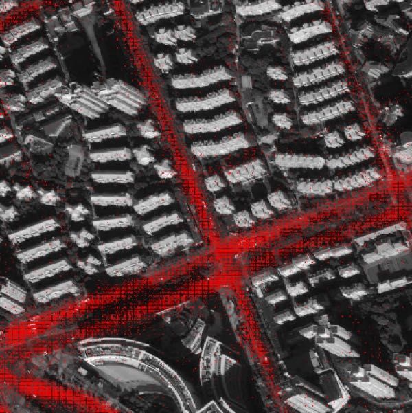
Satellite + GT        GPS Points            GPS only             Image only      Image+GPS (plain)   Image+GPS (ours)

(a)
 BJ

(b)
 BJ

(c)
 BJ

(d)
 SH

(e)
 SH

Figure 10: Prediction results using different methods on Beijing and Shanghai testing datasets trained on Beijing dataset only

occlusion and other image issues can cause poor perfor-               tation techniques, our GPS data augmentation is very ef-
mance. Both image and GPS input give the best results, and            fective against overfitting, and thus our method performs
our enhancement techniques give a bit cleaner output. As              much better in new testings areas than other models. In
examples, the areas pointed by red arrows show false posi-            our experiences, aerial imagery works best for residential
tives removed with our model using GPS data. The one in               roads detection because they are relatively simple, numer-
the first row is a railway and the one in the third row is from       ous, and infrequently traveled. In contrast, GPS data can
GPS noise. The red square shows an area with dense tree               recover arterial roads with ease even for complicated high-
canopy and relatively sparse GPS samples. Only the combi-             way systems and under severe image occlusion. Therefore,
nation of image and GPS data extracts a relatively complete           the two data sources well complement each other for road
road network.                                                         extraction tasks.

6. Conclusion                                                         Acknowledgement
   With large-scale crowdsourced GPS datasets, fusing                    We thank anonymous reviewers for valuable feedback.
GPS data with aerial image input gives much better road               This research is supported by NSFC General Program
segmentation results than using images or GPS data alone              41771481, Shanghai Science and Technology Commission
with deep neural net models. Inspired by image augmen-                program 17511104502, and a gift fund from Facebook.

                                                                  8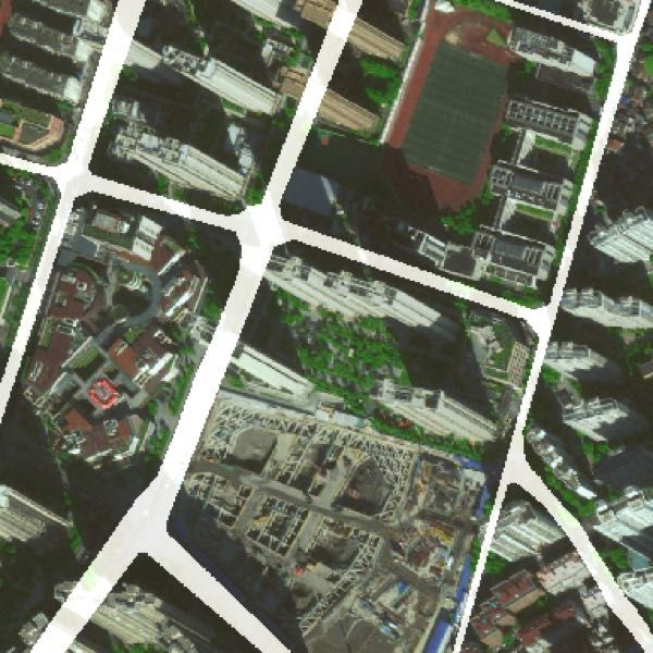
References                                                                     tional conference on Knowledge discovery and data mining,
                                                                               2012. 2, 5, 6
 [1] AI-assisted road tracing. wiki.openstreetmap.org/
                                                                        [16]   G. Máttyus, W. Luo, and R. Urtasun. Deeproadmapper: Ex-
     wiki/AI-Assisted_Road_Tracing. 1, 2
                                                                               tracting road topology from aerial images. In The IEEE In-
 [2] Gaode Map. www.amap.com. 5                                                ternational Conference on Computer Vision (ICCV), 2017.
 [3] OpenStreetMap. www.openstreetmap.org. 1, 2                                2, 6
 [4] S. Aksoy, B. Ozdemir, S. Eckert, F. Kayitakire, M. Pesarasi,       [17]   H. Mayer, S. Hinz, U. Bacher, and E. Baltsavias. A test of au-
     O. Aytekin, C. C. Borel, J. Cech, E. Christophe, S. Duzgun,               tomatic road extraction approaches. International Archives
     et al. Performance evaluation of building detection and dig-              of Photogrammetry, Remote Sensing, and Spatial Informa-
     ital surface model extraction algorithms: Outcomes of the                 tion Sciences, 36(3):209–214, 2006. 1, 2
     prrs 2008 algorithm performance contest. In IAPR Workshop          [18]   V. Mnih. Machine Learning for Aerial Image Labeling. PhD
     on Pattern Recognition in Remote Sensing. IEEE, 2008. 1, 2                thesis, University of Toronto, 2013. 2, 6
 [5] F. Bastani, S. He, S. Abbar, M. Alizadeh, H. Balakrishnan,         [19]   V. Mnih and G. E. Hinton. Learning to label aerial images
     S. Chawla, S. Madden, and D. DeWitt. Roadtracer: Auto-                    from noisy data. In International conference on machine
     matic extraction of road networks from aerial images. In                  learning (ICML), 2012. 1, 2
     Computer Vision and Pattern Recognition (CVPR), 2018. 2,           [20]   A. J. Mosinska, P. Marquez Neila, M. Kozinski, and P. Fua.
     6                                                                         Beyond the pixel-wise loss for topology-aware delineation.
 [6] J. Biagioni and J. Eriksson. Map inference in the face of                 In Computer Vision and Pattern Recognition (CVPR), 2018.
     noise and disparity. In SIGSPATIAL Conference on Geo-                     2
     graphic Information Systems (GIS), 2012. 2                         [21]   P. Newson and J. Krumm. Hidden markov map matching
 [7] A. Chaurasia and E. Culurciello. Linknet: Exploiting en-                  through noise and sparseness. In SIGSPATIAL Conference
     coder representations for efficient semantic segmentation.                on Geographic Information Systems (GIS), 2009. 7
     In Visual Communications and Image Processing (VCIP),              [22]   D. Patel. Osm at facebook. State of the Map, 2018. 1, 2
     2017. 4, 6                                                         [23]   S. Rogers, P. Langley, and C. Wilson. Mining gps data to
 [8] L.-C. Chen, G. Papandreou, I. Kokkinos, K. Murphy, and                    augment road models. In ACM SIGKDD international con-
     A. L. Yuille. Deeplab: Semantic image segmentation with                   ference on Knowledge discovery and data mining, 1999. 2
     deep convolutional nets, atrous convolution, and fully con-        [24]   O. Ronneberger, P. Fischer, and T. Brox. U-net: Convo-
     nected crfs. IEEE transactions on pattern analysis and ma-                lutional networks for biomedical image segmentation. In
     chine intelligence, 40(4):834–848, 2018. 2, 4, 6                          International Conference on Medical image computing and
 [9] J. J. Davies, A. R. Beresford, and A. Hopper. Scalable, dis-              computer-assisted intervention, pages 234–241. Springer,
     tributed, real-time map generation. IEEE Pervasive Comput-                2015. 2, 4, 6
     ing, 5(4):47–54, 2006. 2, 5, 6                                     [25]   S. Schrödl, S. Schrödl, K. Wagstaff, S. Rogers, P. Langley,
[10] I. Demir, K. Koperski, D. Lindenbaum, G. Pang, J. Huang,                  and C. Wilson. Mining GPS traces for map refinement. Data
     S. Basu, F. Hughes, D. Tuia, and R. Raskar. Deepglobe                     Mining Knowledge Discovery, 9(1):59–87, 2004. 2
     2018: A challenge to parse the earth through satellite im-         [26]   Z. Shan, H. Wu, W. Sun, and B. Zheng. Cobweb: a robust
     ages. In Computer Vision and Pattern Recognition (CVPR)                   map update system using gps trajectories. In ACM Interna-
     Workshops, 2018. 2, 4                                                     tional Joint Conference on Pervasive and Ubiquitous Com-
[11] B. Huang, K. Lu, N. Audebert, A. Khalel, Y. Tarabalka,                    puting (UbiComp), 2015. 2
     J. Malof, A. Boulch, B. Le Saux, L. Collins, K. Bradbury,          [27]   E. Shelhamer, J. Long, and T. Darrell. Fully convolutional
     et al. Large-scale semantic classification: outcome of the                networks for semantic segmentation. IEEE transactions on
     first year of inria aerial image labeling benchmark. In IEEE              pattern analysis and machine intelligence, 39(4):640–651,
     International Geoscience and Remote Sensing Symposium                     2017. 2, 4
     (IGARSS), 2018. 2                                                  [28]   T. Sun, Z. Di, and Y. Wang. Combining satellite imagery and
[12] S. Karagiorgou, D. Pfoser, and D. Skoutas. A layered ap-                  gps data for road extraction. 2018. SIGSPATIAL Conference
     proach for more robust generation of road network maps                    on Geographic Information Systems (GIS) workshop. 2
     from vehicle tracking data. ACM Transactions on Spatial            [29]   M. Trifunovic. Robot tracers - extraction and classification
     Algorithms and Systems (TSAS), 3(1):3, 2017. 2                            at scale using & cntk. State of the Map, 2018. 1, 2
[13] Y. LeCun, L. Bottou, Y. Bengio, and P. Haffner. Gradient-          [30]   F. van Diggelen. Gnns accuracy: Lies, damn lies, and statis-
     based learning applied to document recognition. Proceed-                  tics. GPS World, pages 26–32, 2007. 3
     ings of the IEEE, 86(11):2278–2324, 1998. 2                        [31]   M. Volpi and D. Tuia. Dense semantic labeling of sub-
[14] P. Li, Y. Zang, C. Wang, J. Li, M. Cheng, L. Luo, and Y. Yu.              decimeter resolution images with convolutional neural net-
     Road network extraction via deep learning and line integral               works. IEEE Transactions on Geoscience and Remote Sens-
     convolution. In IEEE International Geoscience and Remote                  ing, 55(2):881–893, 2017. 2
     Sensing Symposium (IGARSS), 2016. 2                                [32]   S. Wang, M. Bai, G. Mattyus, H. Chu, W. Luo, B. Yang,
[15] X. Liu, J. Biagioni, J. Eriksson, Y. Wang, G. Forman, and                 J. Liang, J. Cheverie, S. Fidler, and R. Urtasun. Torontoc-
     Y. Zhu. Mining large-scale, sparse gps traces for map infer-              ity: Seeing the world with a million eyes. In International
     ence: comparison of approaches. In ACM SIGKDD interna-                    Conference on Computer Vision (ICCV), 2017. 2

                                                                    9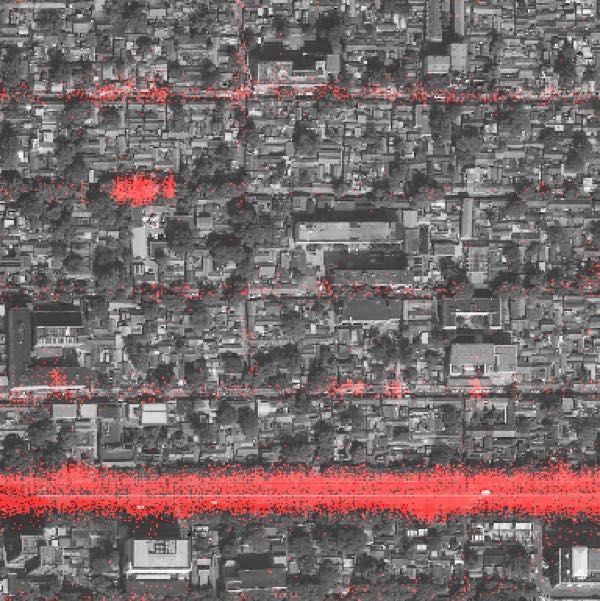
[33] Y. Wang. Scaling Maps at Facebook. In SIGSPATIAL Con-
     ference on Geographic Information Systems (GIS), 2016.
     keynote. 2
[34] Y. Wang, X. Liu, H. Wei, G. Forman, C. Chen, and Y. Zhu.
     Crowdatlas: Self-updating maps for cloud and personal use.
     In International Conference on Mobile Systems, Applica-
     tions, and Services (MobiSys), 2013. 1, 2
[35] G.-S. Xia, X. Bai, J. Ding, Z. Zhu, S. Belongie, J. Luo,
     M. Datcu, M. Pelillo, and L. Zhang. Dota: A large-scale
     dataset for object detection in aerial images. In Computer
     Vision and Pattern Recognition (CVPR), 2018. 2
[36] N. Yokoya, P. Ghamisi, J. Xia, S. Sukhanov, R. Heremans,
     I. Tankoyeu, B. Bechtel, B. Le Saux, G. Moser, and D. Tuia.
     Open data for global multimodal land use classification: Out-
     come of the 2017 ieee grss data fusion contest. IEEE Jour-
     nal of Selected Topics in Applied Earth Observations and
     Remote Sensing, 11(5):1363–1377, 2018. 2
[37] J. Yuan and A. M. Cheriyadat. Image feature based gps trace
     filtering for road network generation and road segmentation.
     Machine Vision and Applications, 27(1):1–12, 2016. 2
[38] Z. Zhengxin, L. Qingjie, and W. Yunhong. Road extraction
     by deep residual u-net. In IEEE GEOSCIENCE AND RE-
     MOTE SENSING LETTERS, 2017. 6
[39] L. Zhou, C. Zhang, and M. Wu. D-linknet: Linknet with
     pretrained encoder and dilated convolution for high resolu-
     tion satellite imagery road extraction. In Computer Vision
     and Pattern Recognition (CVPR) Workshops, 2018. 4, 6
[40] X. X. Zhu, D. Tuia, L. Mou, G.-S. Xia, L. Zhang, F. Xu, and
     F. Fraundorfer. Deep learning in remote sensing: a compre-
     hensive review and list of resources. IEEE Geoscience and
     Remote Sensing Magazine, 5(4):8–36, 2017. 2, 6

                                                                     10
You can also read