Sound pressure level spectrum analysis by combination of 4D PTV and ANFIS method around automotive side view mirror models
←
→
Page content transcription
If your browser does not render page correctly, please read the page content below
www.nature.com/scientificreports
OPEN Sound pressure level spectrum
analysis by combination
of 4D PTV and ANFIS method
around automotive side‑view
mirror models
Dong Kim1, Arman Safdari2 & Kyung Chun Kim3*
This paper proposes a data augmentation method based on artificial intelligence (AI) to obtain sound
level spectrum as predicting the spatial and temporal data of time-resolved three-dimensional Particle
Tracking Velocimetry (4D PTV) data. A 4D PTV has used to measure flow characteristics of three side
mirror models adopting the Shake-The-Box (STB) algorithm with four high-speed cameras on a robotic
arm for measuring industrial scale. Helium filled soap bubbles are used as tracers in the wind tunnel
experiment to characterize flow structures around automobile side mirror models. Full volumetric
velocity fields and evolution of vortex structures are obtained and analyzed. Instantaneous pressure
fields are deduced by solving a Poisson equation based on the 4D PTV data. To predict spatial and
temporal data of velocity field, artificial intelligence (AI)-based data prediction method has applied.
Adaptive Neural Fuzzy Inference System (ANFIS) based machine learning algorithm works well to find
4D missing data behind the automobile side mirror model. Using the ANFIS model, power spectrum
of velocity fluctuations and sound level spectrum of pressure fluctuations are successfully obtained to
assess flow and noise characteristics of three different side mirror models.
Most drivers know that they must turn up the volume to listen to their favorite radio channels on the highway
and speak louder to talk to the passenger. This is a direct result of the turbulence that induced pressure fluctuation
around window. The pressure fluctuation creates vibrations of window glass plates, which generate some of the
internal noise through the air inside the vehicle. There are five types of wind noise sources: turbulent boundary
layers, separated and reattaching flow, cavity flow, vortex shedding, and leak (or aspiration) noise1. Side view
mirrors can contribute to significant interior noise in the automobile cabins. The vortices induced by the mirrors
produce powerful exterior noise and hydrodynamic impingement, which excite the downstream windows. The
interior noise can be reduced by suppressing the turbulent flow separation on the mirrors.
To measure noise sources, wind tunnel testing is still a common method in the automotive industry1–8. Vari-
ous turbulent structures around exterior mounted vehicle mirrors have been investigated experimentally by
Rinoshika et al.9. In addition, Khalighi et al.10 conducted Particle Image Velocimetry (PIV) and pressure meas-
urements behind the two outer side view mirrors of the vehicle in the wake region. Kim et al.7 measured surface
flow and wake structure of passenger car side view mirror. In order to measure velocity and pressure which are
important properties for determining aerodynamic performance, point measurement methods such as a pressure
transducer and a hot-wire are adopted or 2D planar PIV measurement is being conducted. In the case of pressure
measurement, it cannot identify the nature of the noise mechanism as well as time and effort, as the microphone
arrangement is installed to measure floating noise and to use a trial-and-error method to modify features. Far
field data using microphone arrays do not provide enough information on the source mechanism, so it relies on
a numerical analysis or source model to understand additional information from the source region. In addition,
most PIV measurements are limited to 2D. Obtaining pressure field after performing 3D flow analysis by direct
numerical simulation (DNS) or large eddy simulation (LES) is difficult to apply to a complex shape or a high
1
Rolls‑Royce University Technology Centre, Pusan National University, Busan 46241, Republic of
Korea. 2Department for Management of Science and Technology Development, Ton Duc Thang University, Ho
Chi Minh City, Vietnam. 3School of Mechanical Engineering, Pusan National University, Busan 46241, Republic of
Korea. *email: kckim@pusan.ac.kr
Scientific Reports | (2021) 11:11155 | https://doi.org/10.1038/s41598-021-90734-1 1
Vol.:(0123456789)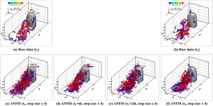
www.nature.com/scientificreports/
Reynolds number due to computational cost and turbulence model. In addition, the results of the numerical
analysis must be verified by experiment.
Today, pressure from PIV techniques provide an alternative to the complex devices of a wind tunnel model
with pressure tap for pressure measurement11–13. Once velocity material derivatives is accurately calculated, the
established time-resolved pressure from PIV procedure solves the incompressible Poisson equation for pressure.
Due to uncorrelated random errors in consecutive PIV snapshots, recent studies have employed a Lagrangian
tracking14 approach to obtain the velocity material derivative from a series of consecutive time-resolved velocity
measurements. The combination of tracer particle technology for large-scale wind tunnel experiments (helium
filled soap bubbles (HFSB)) and coaxial volumetric velocimetry with the advancements in 3D particle motion
analysis (Shake-the-Box) has shown the potential to evaluate the velocity and pressure field in volumes of several
liters15. An accurate determination of the velocity material derivative in turbulent flows requires full 3D evalua-
tion of the velocity and acceleration field, which is currently possible by high-speed, high-resolved experiment.
Turbulent flow generally involves multidimensional physics, including space and time, which have high
dimensions with rotating and transforming intermittent structures. This feature provides an opportunity for
the application of artificial intelligence (AI) methods, such as machine learning to predict the modeling and
analysis of turbulent flow. Neural networks are popular in a range of areas, including self-driving cars and weather
forecasts. Recently, there have been interesting studies on the use of neural networks for fluid dynamics16–25,
including turbulence m odeling18,21. The Adaptive Neuro-Fuzzy Inference System (ANFIS) method can learn
many physical models and can be very useful in chemical engineering, pharmaceuticals, and industry26. This
method calculates the changes in linguistic concepts into mathematical or computational ones, which can alter
its behavior in different environments and learn to calculate the behavior of many processes that may be uncer-
tain. Neuro-fuzzy computing methods are an example of such techniques. These methods take advantages of
machine learning capability of artificial neural networks, and fuzzy inference systems to make reasonable deci-
sions according to the if–then rules27.
This paper proposes an AI-based data prediction technique combining the 4D robotic PTV measurement
data and an ANFIS framework for fluid dynamic research. The main objectives of this study is intended to
establish the ANFIS as an auxiliary tool to collaborate with the 4D PTV approach as well as sound pressure level
spectrum analysis. To estimate turbulent pressure field from the time-resolved three-dimensional velocity field
data obtained by 4D PTV method, high-resolution of temporal and spatial data should be prepared since second
derivatives are included in Navier–Stokes equation. For the purpose, we used a machine learning model. For
a good prediction, ground-truth data is necessary. The 4D PTV data include some error vectors, but they are
ground truth data obtained by experiments. In addition, as far as the authors aware of, there is no study to use the
AI algorithms for developing the sound pressure level spectrum relationship between the experimental results.
We use experimental data of fluid flow for different time steps as a data set, and with the ANFIS method. After
training all patterns of fluid, the AI predicts missing times with the experimental method, which has not been
used in the training method. Learning 3D or 4D flow patterns through AI can result in excellent generalization
ability of the resulting model and a decrease in error and noise because it learns statistical data based on the
neural network algorithm, which can be stored in a database. The instantaneous pressure field was estimated by
solving the Poisson equation using 4D PTV data. The ANFIS model was trained using the time-resolved three-
dimensional PTV data measured in the wake region of the side-view mirror model for automobiles as a ground
truth. To determine the three-dimensional flow structure and noise characteristics of the side-view mirror model,
the instantaneous velocity and pressure field were deduced from the ANFIS model. Vortex shedding phenomena
and flow-induced noise are discussed based on the power spectrum and sound pressure level spectra.
Methods
4D Lagrangian robotic PTV measurements of side‑view mirror models. The side-view mirror of
a vehicle should be designed with a shape that minimizes the aerodynamic noise and aerodynamic r esistance28.
Previous studies examined the vortex characteristics of a vehicle’s side-view mirror using a computational fluid
analysis technique or measured the time-average velocity field of a wake flow field using a two-dimensional
PIV technique4. The flow noise generated in the side-view mirror was measured on the wall surface using a
microphone array, but the relationship between the characteristics of the flow structure and noise needs to be
investigated29. For the optimal design of the automobile side-view mirror, information on the pressure field of
flow and the 3D flow field are required.
In this study, the time-resolved three-dimensional velocity field of the flow passing through the side-view
mirror model was measured using a robotic PTV equipped with four high-speed cameras and the Shake-The-Box
(STB) algorithm30. To characterize the flow structures around an automotive side-view mirror model, helium-
filled soap bubbles were used as tracers in the wind tunnel experiment as shown in Fig. 1. The coaxial volumet-
ric velocimeter (CVV) probe was installed on a collaborative robotic arm UR5 from Universal R obots31. The
robotic arm provided three rotation and three translation axes movement. The accuracy of the translation was
approximately 0.1 mm. The robotic arm’s position could be controlled and simulated using RoboDK software.
The light source was a Quantronix Darwin Duo Nd:YLF diode-pumped laser (λ = 527 nm, 2 × 25 mJ pulse energy
at 1 kHz). The velocimeter probe consisted of four CMOS cameras equipped with objectives with a 4 mm focal
length. The spatial resolution of image sensor is 640 × 452 p ix2 to 300 × 200 mm2. The cameras were integrated
within an oval body (LaVision MiniShaker Aero). For volume illumination, the laser light was transmitted with
an optical fiber towards the CVV head, where the beam was expanded with a spherical lens31. The mirror model
has an aspect ratio of H/W = 2. L in the streamwise direction (x-axis), where W is the spanwise direction (y-axis),
and H is the direction normal to the wall (z-axis). The experiment was conducted with a free-stream velocity of
13 m/s and a Reynolds number of 85,752. Table 1 lists the experimental conditions.
Scientific Reports | (2021) 11:11155 | https://doi.org/10.1038/s41598-021-90734-1 2
Vol:.(1234567890)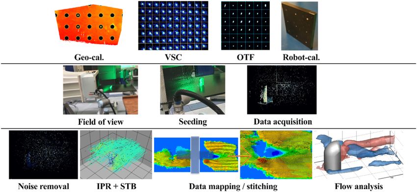
www.nature.com/scientificreports/
Figure 1. Experimental setup for time-resolved Lagrangian particle tracking velocimetry and side-view mirror
models used in this study.
Velocity of free-stream 13 m/s
Reynolds number 85,752
Boundary layer thickness at x/H = − 1 δ/H ≈ 0.2
Height of model (H) 10 cm
Aspect ratio of the model H/W = 2
R/H = 0.4 (top)
Streamlined curvatures of the model
R/H = 0.25 (front)
Image acquisition frequency 867 Hz
Spread angle of illumination 40o
Blockage ratio 1.4%
Table 1. Experimental conditions for the 4D PTV measurements.
The measurements were conducted in an open jet open-return-circuit wind tunnel with a square contraction
ratio of 1:4 and a 60 × 60 c m2 cross-section. The velocity profile was measured in the free-stream region using
2D time-resolved PIV. The side-view mirror model was immersed in the turbulent boundary layer in the free-
stream region with respect to the model height at δ/H ≈ 0.2. The field of view was checked using the reflectance
produced by the laser beams. The probe was repositioned if the reflection exceeded 256 counts. If both the field
of view and reflections were acceptable, the viewing information could be stored in a Davis 10 program. A Fluid
Supply Unit was operated to seed with the tracer particles, and the seeding concentration was evaluated by a
visual inspection before the data are acquired. Once the seeding concentration was satisfactory, the data were
acquired (20,000 images at 867 Hz).
Scientific Reports | (2021) 11:11155 | https://doi.org/10.1038/s41598-021-90734-1 3
Vol.:(0123456789)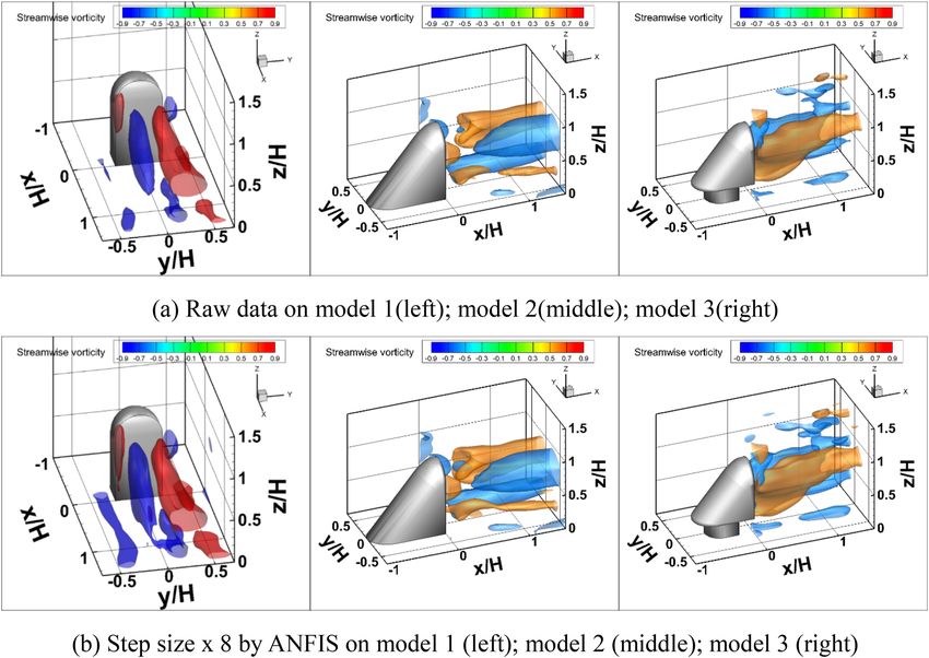
www.nature.com/scientificreports/
Figure 2. Schematic diagram of data acquisition using the robotic 4D PTV; 1st row represents calibration
process; 2nd row represents data recording process; 3rd row represents data reduction and post-processing.
Figure 2 presents a schematic diagram of the working principles of robotic volumetric PTV schematically. The
calibration process included the following: geometrical c alibration32, volume self-calibration33, optical transfer
function34, and robot c alibration31. After calibration, the robotic arm was positioned to define the field of view
and move the velocimeter to the desired position via a robot-control tablet. Post-processing for data reduction is
summarized as follows. Raw images were pre-processed using Butterworth filters35 to eliminate the background
noise and reflection. Pre-processed images were provided as an input to the STB a lgorithm14 to reconstruct
the particle track. The data from the camera reference system XYZcamera were converted to the global reference
system XYZglobal, which was aligned with the free stream. The representation of Lagrangian tracking was then
mapped to a structured grid using a binning process. The grid elements of the interrogation volume or bin were a
20 × 20 × 20-mm3 cube with 75% overlapping, and a velocity vector field with a 5-mm vector pitch was produced.
The maximum uncertainty of the in-plane position given by the standard deviation of x and y is estimated on
the order of 0.5 mm, while the value for the depth position is 2.5 mm, as expected, according to the small tomo-
graphic aperture of the camera system.
Pressure field evaluation from 4D PTV data. Instantaneous pressure, p, can be calculated by solving
the Poisson e quation11.
Du
∇ 2 p = ∇ · −ρ + µ∇ 2 u (1)
Dt
with the von Neumann boundary conditions on all volume boundaries except for the top side. At the top side,
a Dirichlet boundary condition is specified from the Bernoulli equation. At the boundaries, the von Neumann
condition was applied, as proposed by Ebbers and Farnebäck12. The application of the von Neumann boundary
condition will yield the solution of the pressure field up to a finite integration constant. To eliminate the latter,
the Dirichlet condition needs to be specified at a known reference location. For the present data, the pressure
far upstream of the test object was matched to the expected free-stream pressure. Visualization of the vorticity
distribution confirmed the irrotational flow at the top boundary of the measurement. The material derivative in
Eq. (1) was evaluated using the Lagrangian technique13.
Data prediction using Adaptive Neuro‑Fuzzy Inference System (ANFIS). Figure 3 shows the sim-
ple structure of the ANFIS model. The training process can be mathematically regarded as an optimization prob-
lem to determine the weighting factor. Given the input data set x and the desired output data set y , ANFIS aim
to find the optimal weight w in a machine-learned model F that acts as a nonlinear regression function such that
F(x; w) ≈ y . In the present case, x and F(x; w) represent the low-resolution and reconstructed high-resolution
data, respectively. The weight w is optimized between the desired high-resolution output y and the ML model
output F(x; w) is minimized. The model was used to predict the time-resolved 3D flow characteristics of the
side-mirror model with two membership functions as input. Four inputs of the x, y, z coordinates, and time t
were applied to obtain the time-resolved three velocity components, and the output was the instantaneous 3D
velocity components and pressure. The first-order Sugeno fuzzy model with fuzzy if–then rules were also used.
The output of the ith node in layer l is O1,i.
Layer 1: Each node i in the first layer is an adaptive node with a node function.
Scientific Reports | (2021) 11:11155 | https://doi.org/10.1038/s41598-021-90734-1 4
Vol:.(1234567890)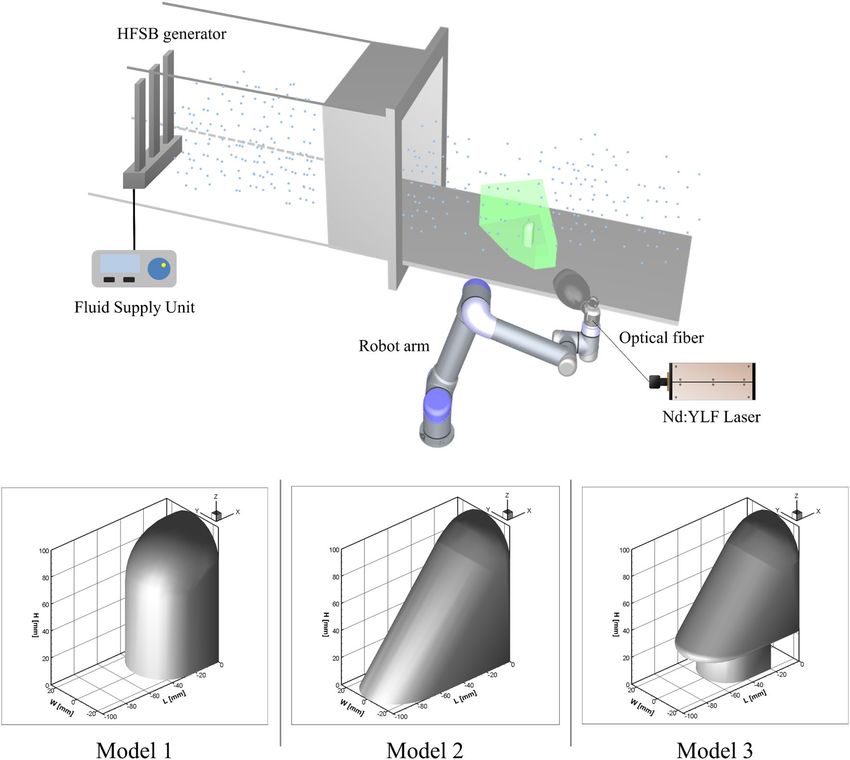
www.nature.com/scientificreports/

                                  Figure 3.  ANFIS structure with a four-input first-order Sugeno fuzzy model in MATLAB 2017a. 4 inputs of
                                  coordinates system, and time t were applied and the output was the instantaneous 3D velocity components and
                                  pressure.

                                                                           O1,i = µAi (x), for i = 1, 2, or
                                                                                                                                                     (2)

                                                                           O1,i = µBi−2 y , for i = 3, 4 or
                                                                           O1,i = µCi−4 (z), for i = 5, 6
                                  where x, y, and z are the inputs to node i, and Ai , Bi−2, and Ci−4 are the associated linguistic labels. Ol,i is any
                                  suitable parameterized membership function of a fuzzy set. A fuzzy set is described entirely using its member-
                                  ship function. A generalized bell function was applied because of its great capabilities for the generalization of
                                  nonlinear parameters:
                                                                                                    1
                                                                                µA (x) =
                                                                                                    x−ci
                                                                                                           2bi                                      (3)
                                                                                           1+        ai

                                  where {ai , bi , ci } is a variable set. The bell-shaped function differs according to the values of the variables, so
                                  it shows various kinds of membership functions for fuzzy set A. The variables in the first layer are known as
                                  premise variables.
                                      Layer 2: Each node in the second layer is a fixed one, and its output is the result of all incoming signals:

                                                                                                                                                     (4)

                                                                          O2,i = wi = µAi (x)µBi y µCi (z), i = 1, 2, 3

                                  Every node output indicates the firing strength of a rule.
                                      Layer 3: Each node in the third layer is a fixed one. The ith node calculates the proportion of the firing strength
                                  of the ith rule in the sum of the firing strength of all rules:
                                                                                              wi
                                                                            O3,i = wi =
                                                                                           w1 + w2
                                                                                                   , i = 1,2,3                                       (5)

                                  For convenience, the outputs of this layer are called the normalized firing strengths.
                                     Layer 4: Each node in this fourth layer is an adaptive node with a node function:
                                                                     O4,i = wi fi = wi ui = wi (pi x + qi y + ri z + si t + hi )                     (6)
                                  where wi is the normalized firing strength from the third layer, and pi , qi , ri , si is node’s variable set. In this

                                  layer, the variables are referred to as consequent parameters.
                                       Layer 5: In the fifth layer, the single node is a fixed node that calculates the total output as the summation of
                                  all incoming signals:

                                                                             O5,i =       wi ui =     wi ui /      wi                                (7)
                                                                                   i            i                 i

                                     Different variables in the ANFIS structures were identified using a hybrid learning method. In the forward
                                  pass, functional signals moved forward until they reached Layer 4. The consequent variables were identified by
                                  the least-squares estimate. In the backward pass, the error rates moved backward. The gradient descent updates
                                  the premise parameters.
                                     The accuracy and performance of the ANFIS method were evaluated based on the statistical parameters.
                                  The root mean square error (RMSE) was used to compare the difference between the ANFIS prediction values
                                  and the measured data:

Scientific Reports |   (2021) 11:11155 |               https://doi.org/10.1038/s41598-021-90734-1                                                      5

                                                                                                                                                  Vol.:(0123456789)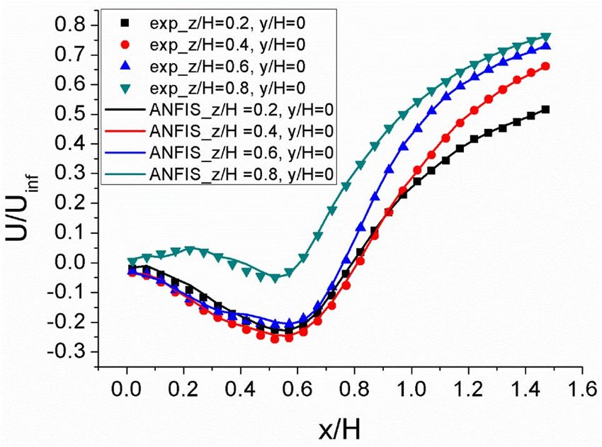
www.nature.com/scientificreports/
Figure 4. Flow chart of the ANFIS prediction and data prediction of 4D PTV data. The values of the
convergence criteria were based on R2 > 0.99 and RMSE < 0.01.
Figure 5. Training domain for ANFIS prediction (red box). The selected domain was used to observe the flow
characteristics of the wake region with ranges of 0 < x/H < 1.5, − 0.7 < y/H < 0.7, and 0 < z/H < 1.3.
n
i=1 (Oi − Pi )2
RMSE = (8)
n
where O, P, and n are the measured data, predicted data, and number of data, respectively. The correlation coef-
ficient (R2) is a criterion that illustrates how well the ANFIS data fit the measured data.
n n n
2
(9)
R = Oi − Oi Pi − Pi 2 Oi − Oi Pi − Pi
i=1 i=1 i=1
Figure 4 presents a flow chart of the ANFIS prediction process. The first step was to load the measured 4D
PTV data and set the domain of the desired area. In Fig. 5, the red box shows the ANFIS prediction domain.
The selected domain was used to observe the flow characteristics of the wake region with ranges of 0 < x/H < 1.5,
− 0.7 < y/H < 0.7, and 0 < z/H < 1.3. Subsequently, the ANFIS parameters were applied to train the AI. The ANFIS
generation parameters include the percentage of the training and testing data, number of membership functions,
type of input membership function, and type of output membership function. To train the ANFIS structure, the
parameters included the number of epochs, error goal, initial step size, and the decrease and increase rates of the
Scientific Reports | (2021) 11:11155 | https://doi.org/10.1038/s41598-021-90734-1 6
Vol:.(1234567890)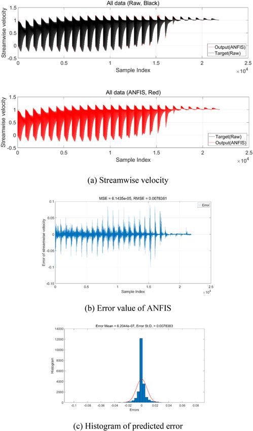
www.nature.com/scientificreports/
Parameters Input
28 × 30 × 26 × 6,666 = 145,585,440 nodes
Input
(x/H, y/H, z/H, t)
Target u, v, w, p
Training (70%)
Percentage of training and testing data
Testing (30%)
Type of input membership function Generalized bell function
Number of input membership functions 2, 3, 4, 5, 6, 7
Number of fuzzy rules 16, 81, 256, 625, 1296, 2401
1000
(The number of input membership function = 2, 3, 4)
Epochs
300
(The number of input membership function = 4, 5, 6)
Table 2. ANFIS parameters used for convergence and sensitivity test.
Figure 6. Convergence of the ANFIS model with respect to the number of epochs. The number of epochs
reached 300, the degree of convergence of the model was satisfactory.
step size. After setting up the ANFIS parameters, ANFIS training can be started using the measured data, and
the convergence can be checked. The values of the convergence criteria were based on R 2 > 0.99 and RMSE < 0.01.
If the values of the convergence criteria are satisfactory, the obtained ANFIS results were applied to the testing
data. After checking the convergence of the test data, the ANFIS model was used to predict the data of the 4D
PTV data. A good ANFIS model can make entirely new predictions without data in the training process. When
a new ANFIS mesh domain is created, the required results can be predicted using the developed ANFIS model.
The training cases were classified into three main categories based on the input membership function, percentage
of training and testing data, and number of epochs.
Table 2 lists the ANFIS parameters for the input membership function. The experimental results on velocity
components and pressure of the side mirror model were used for the sensitivity and accuracy test of the ANFIS
model. The numbers of nodes of x, y, and z in the domain were the same as those of the experimental velocity
field. On the other hand, 6,666 images (every fourth time-resolved data (289 Hz) were used for training because
of the memory limit of the computer. The maximum number of input nodes was 145,585,440. In this case, 70%
of the experiment results were used as input to the ANFIS for training. The remaining data were used as testing
data to check the prediction results. The convergence was checked while increasing the number of input mem-
bership functions. The first three cases had two, three, and four input membership functions with 1000 epochs.
After checking how many epochs were satisfactory and converged, the last three cases were examined with five,
six, and seven input membership functions, and the epochs were reduced to 300.
Figure 6 shows the convergence tendencies of the ANFIS model with respect to the number of epochs. n is
the number of input membership functions. When the number of input membership functions was two, three,
and four, the RMSE values were 0.11, 0.05, and 0.02 after 1000 epochs, respectively. When the number of epochs
reached 300, the degree of convergence of the model was satisfactory. When the number of input membership
functions was five, six, and seven, the RMSE values were 0.02, 0.01, and 0.005, respectively.
Figure 7 shows the RMSE value and computation time of the ANFIS model with respect to the number of
input membership functions. The computations were performed on a computer with an Intel Core i5-8400 CPU
2.80 GHz and 16.0 GB of RAM. With 300 epochs and six input membership functions, the ANFIS training took
approximately eight hours and satisfied the convergence criterion of RMSE < 0.01. The RMSE value decreased
Scientific Reports | (2021) 11:11155 | https://doi.org/10.1038/s41598-021-90734-1 7
Vol.:(0123456789)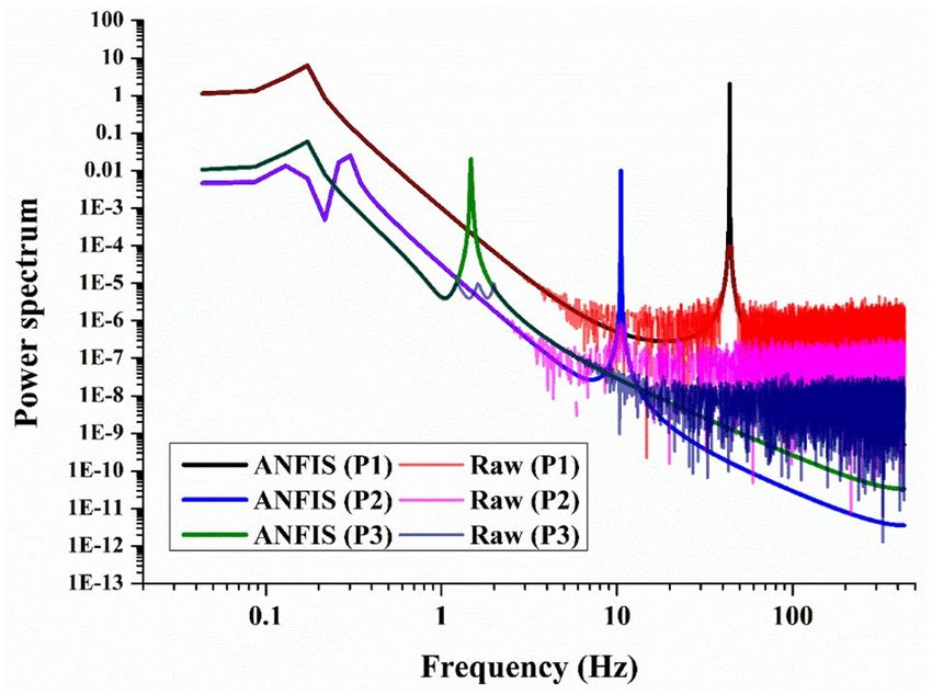
www.nature.com/scientificreports/
Figure 7. Root mean square error (RMSE) and computation time of the ANFIS model with respect to the
number of input membership functions.
with increasing number of input membership functions. On the other hand, the RMSE value decreased when the
number of inputs exceeded seven, but the rate of decrease of the RMSE was very low, and the computational time
increased suddenly, which is inefficient. Therefore, six functions and 300 epochs are efficient for convergence.
Figure 8 shows the ANFIS model’s error of average streamwise velocity compared with measurement data
for model 1. Figure 8a shows the comparison with measurement data (target) and ANFIS result (output). For
training, the RMSE value of streamwise velocity is 0.0078. This result shows that the error between the predicted
data and measurement value is less than 0.78% for streamwise velocity component. Consequently, this shows
the high degree of linear dependence R 2 between the ANFIS and measurement result in the training process.
Consequently, the ANFIS model can accurately predict the 4D PTV velocity and aerodynamics with an error of
less than 0.78%. This error can be reduced with more input membership function.
Results and discussion
The ANFIS method can predict the time-resolved three-dimensional velocity field of the side mirror model
with less computational time and provide high temporal and spatial resolution. The number of raw data in the
x/H, y/H, and z/H mesh coordinates was 28 × 30 × 26 nodes, which have 21,840 data. This coordinate had a step
size of 0.05 between the nodes. For ANFIS-based data prediction of 4D PTV, the ANFIS model predicted x/H,
y/H, and z/H from 0 to 1.5, − 0.7 to 0.7, and 0 to 1.3, respectively, with step sizes of 0.00625. This means that the
spatial resolution of the raw data will increase eight-fold. The total number of nodes is 241 × 225 × 209 nodes
(11,333,025 data).
Figure 9 compares the ensemble-averaged streamwise vortex structures between the raw data and ANFIS
data prediction for three different side mirror models. The increase in spatial resolution means that the vorticity,
which is a function of the gradient of velocity and space, can be well distinguished. In the case of the ANFIS
model, the connection of the horseshoe vortex from the bottom of the model was very clear. On the other hand,
in the case of raw data, the horseshoe vortex was broken due to a lack of spatial resolution, as shown in model
1’s result. The sidewall roll-up vortex and trailing vortex pair were also recovered well by ANFIS data prediction.
When the flow was developing downstream, the vortex pair inclined towards the ground plane owing to the
downwash effect. The streamwise trailing vortex pair showed a dipole distribution, counterclockwise rotation
in the left-hand side vortex, and clockwise rotation in the right-hand side vortex. For model 2, the horseshoe
vortex disappeared due to the inclination of the model at the front side, but a trailing vortex formed into a dipole
formation. In the case of the lower vortex pairs of the dipole trailing vortex, the raw data show that the vortex
form is broken. After ANFIS data prediction, this vortex was recovered by the high spatial resolution. For model
3, the horseshoe vortex that occurs at the base of the model is clearer. A horseshoe vortex with small size and
magnitude occurs because the base of the model has the same shape as the reference model.
Figure 10 shows the comparison of normalized average streamwise velocity for experimental result and ANFIS
data prediction of model 1. This result shows the predicted and measured streamwise velocity at the x–y plane
for different z position. According to the line data, the ANFIS data predictions are in good agreement with the
measurement data for all the domain, which is almost same with the PTV results. In comparison to the experi-
mental data, the ANFIS data prediction slightly poor predicts the streamwise velocity in recirculation region.
This is because the absolute velocity magnitude in recirculation region is very low compared with another region.
It is possible to enhance this poor prediction, different ANFIS setting parameters or data filtering are required,
especially the number of input membership function.
The average velocity fields cannot resolve relatively small vortex structures as well as the evolution of the
vortex structures. To take more advantages of the ANFIS data prediction, the instantaneous velocity field of the
side mirror model 1 was used for data prediction.
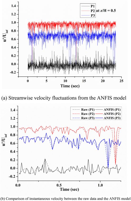
Figure 11 presents the instantaneous streamwise vortex structures in the wake of the side mirror model 1.
Compared to the ensemble-averaged results (Fig. 9a,b), the effects of data prediction were certainly apparent. The
AI-based data prediction results (Fig. 11c,f) showed much smaller vortex structures as a result of the four-fold
Scientific Reports | (2021) 11:11155 | https://doi.org/10.1038/s41598-021-90734-1 8
Vol:.(1234567890)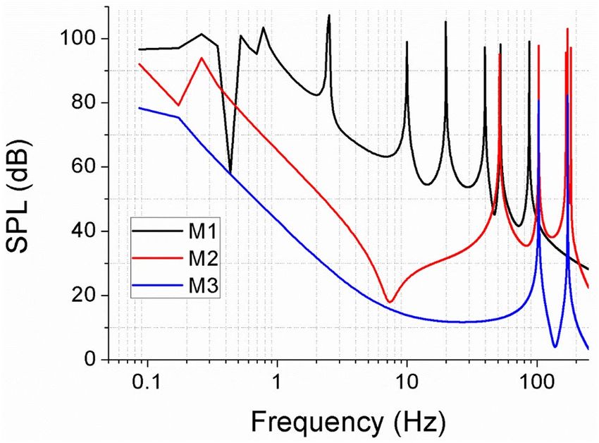
www.nature.com/scientificreports/

                                  Figure 8.  Accuracy of ANFIS model for average streamwise velocity for model 1. (a) Comparison of
                                  streamwise velocity; (b) error of streamwise velocity value; (c) histogram of ANFIS error.

Scientific Reports |   (2021) 11:11155 |             https://doi.org/10.1038/s41598-021-90734-1                                            9

                                                                                                                                      Vol.:(0123456789)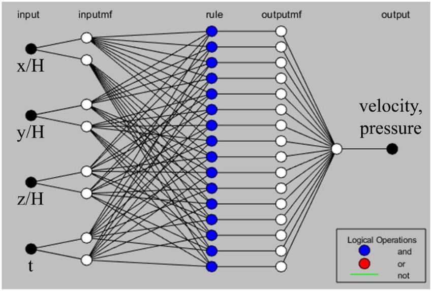
www.nature.com/scientificreports/

                                            Figure 9.  Comparison of the ensemble-averaged 3D streamwise vortex structures between the raw and
                                            predicted data. The spatial resolution of the raw data will increase eight-fold by ANFIS.

                                            Figure 10.  A comparison of normalized average streamwise velocity for experimental result and ANFIS data
                                            prediction of model 1 along the x/H at z/H = 0.2 ~ 0.8, y/H = 0.

                                            increase in the spatial resolution. Moreover, the four-times higher temporal resolution of the ANFIS model
                                            revealed much more small-scale streamwise vortical structures than those from only an enhancement of the
                                            spatial resolution. Compared to the average streamwise vortex structure, the instantaneous vorticity field was
                                            not a symmetrical feature. Clusters of the vortex structure rotating clockwise or counterclockwise were inclined
                                            to the bottom with downwash flow. During the measurement period of Fig. 11c–f, the vortex structures rotating
                                            clockwise were above the vortex structures rotating counterclockwise, but at other times it could be the opposite

          Scientific Reports |   (2021) 11:11155 |              https://doi.org/10.1038/s41598-021-90734-1                                                10

Vol:.(1234567890)
www.nature.com/scientificreports/
Figure 11. Comparison of the instantaneous 3D streamwise vortex structures between the raw and predicted
data. (a,b) Raw data at t1, t2; (c,f) spatial enhancement by ANFIS at t1, t2; (d,e) spatio-temporal enhancement
by ANFIS.
Figure 12. Measurement positions at z/H = 0.5. P1 is in the recirculation zone; P2 is located at the wake shear
layer region; P3 is in the area where the trailing vortex appeared near the central region of the wake after passing
the recirculation zone downstream of the model.
considering that the time-averaged streamwise trailing vortex structure is symmetrical. These data prediction
results provide a better understanding of the small turbulence structures and allow for more in-depth analysis
by recovering the missed data due to the resolution limit of the experiment.
From the ANFIS model with improved temporal and spatial resolution, it was possible to extract the instan-
taneous velocity and pressure fluctuations at a specific location in the flow field. After obtaining the power and
noise level spectrum from the time series data, it was possible to obtain the shedding frequency of the vortex from
the side mirror model and identify the noise source from the fluctuation of the flow pressure. Figure 12 shows
three locations where the velocity and pressure are extracted from the horizontal plane at z/H = 0.5 for model
1. Position 1 (P1) is in the recirculation zone (x/H = 0.2, y/H = − 0.2), where backflow occurs behind the model.
Position 2 (P2) is located at the wake shear layer region (x/H = 0.5, y/H = − 0.3) with a high streamwise velocity.
Position 3 (P3) is in the area where the trailing vortex appeared near the central region (x/H = 1.0, y/H = − 0.1)
of the wake after passing the recirculation zone downstream of the model.
Figure 13a shows the extracted streamwise velocity fluctuations from the ANFIS model at three different
positions on model 1 for the entire measurement time, 22 s. The velocity magnitudes were mostly negative at P1
because the location is within the recirculating zone. The velocity fluctuation at P2 had the highest magnitude
Scientific Reports | (2021) 11:11155 | https://doi.org/10.1038/s41598-021-90734-1 11
Vol.:(0123456789)www.nature.com/scientificreports/
Figure 13. Comparison of the instantaneous streamwise velocity fluctuations between the raw and predicted
data taken at P1, P2, and P3 in the horizontal plane at z/H = 0.5 for model 1.
because the location is just outside of the recirculation zone, where the separated shear layer exists. The time
series of the streamwise velocity at P3 had a lower velocity magnitude than that of P2. On the other hand, the
turbulent intensity of P3 was higher than that of P2. The position was located in the trailing vortex region, which
is inside the wake flow. Figure 13b compares the instantaneous velocity extracted at three different points from
the raw velocity data and the ANFIS model with a four-fold higher temporal resolution than the raw data. For
a better comparison, only 1.5 s were selected. The overall change was consistent with each other, but the ANFIS
model resolved more fluctuations. Every fourth ANFIS result coincided with the raw data because raw data was
used as the ground truth in ANFIS learning.
The dominant characteristics of the external flow over a bluff body were vortex shedding, and flow-induced
noise is closely related to this phenomenon. The shape of the side mirror model was similar to a half-cylinder
and vortex shedding occurred behind the model. Fast Fourier Transform (FFT) analysis was performed with
the velocity signals of Fig. 13a.
Figure 14 shows the power spectra of the streamwise velocity fluctuations extracted at the three points.
Because the power spectrum was obtained only with the fluctuation component of the velocity, the highest power
value came out from position P1, where the fluctuation was the largest, and in the order of P3 and P2. In Fig. 14,
the power spectra obtained using the raw velocity data and the instantaneous velocity extracted from the ANFIS
model were compared. Both coincided with each other in the low-frequency range below 3 Hz, but there were
significant differences in the high-frequency range above 10 Hz. The power spectrum obtained using the raw
data revealed a noisy spectrum with the same mean value above 10 Hz. Because the sampling rate of raw data
was 289 Hz, the spectrum above 145 Hz was meaningless using the Nyquist sampling criteria, and high power at
a lower frequency was derived from aliasing. On the other hand, the ANFIS model had a resolution of 867 Hz.
Therefore, it showed a very clean spectrum in the frequency range below 400 Hz.
The instantaneous velocity field obtained as a result of the AI-based data prediction showed the vortex shed-
ding frequency as a very clear peak. The power spectrum tended to decrease with the power-law as it goes into
higher frequencies. Interestingly, the peak frequency of the spectrum obtained at each point was different because
the structure of the dominant vortex in each position was different. The most prominent frequency peak was
50 Hz measured at the P1 position. This position is closely related to the vortex shedding that occurs on the side
Scientific Reports | (2021) 11:11155 | https://doi.org/10.1038/s41598-021-90734-1 12
Vol:.(1234567890)www.nature.com/scientificreports/
Figure 14. Comparison of the power spectrum from the instantaneous streamwise velocity fluctuation between
the raw and predicted data taken at P1, P2, and P3 in the horizontal plane at z/H = 0.5 for model 1.
Figure 15. Comparison of predicted sound pressure level at P1 for three different side mirror models.
of the semi-cylindrical side mirror model. In the P2 position, periodic vortex shedding of approximately 10 Hz
occurred. This location was related to the abnormality of the trailing vortex structure. In the spectrum at the P3
position, a low-frequency peak of 1.5 Hz, which was not found in the raw data, appeared in the ANFIS model
results. Because the P3 position becomes the point where the recirculating zone ends, it was assumed that it
would be related to the slow meandering phenomenon of the separation bubble.
The pressure fluctuation was quantified to compare the noise of the mirror models at P1. Instantaneous pres-
sure fields were deduced by solving a Poisson equation based on the 4D PTV data. The instantaneous pressure
extracted from the raw data and the ANFIS model with a four-fold higher temporal resolution. The instantaneous
pressure data were converted to sound pressure levels using the following equation and a frequency analysis:
P
SPL = 20 × log10
Pref
P is the instantaneous pressure data, and P ref is the reference sound pressure (20 × 10–6 pa was used for sound
pressure in air).
Figure 15 shows a comparison of the sound pressure level for different side mirror models. The magnitude
of the noise level was highest for model 1, followed by model 2 and model 3 at the same position. The peak of
model 1 was dominant at 10–100 Hz in the low frequency band. This region has strong air resonance, and most
of the noise felt by humans is in this area. At model 1, the peak frequencies were found at 10, 20, 40, 80, and
120 Hz, which are the harmonics based on 10 Hz. At model 2, the peak sound frequencies were observed at 50,
100, and 200 Hz, which are the harmonics of vortex shedding frequency, 50 Hz. At model 3, peaks appeared at
Scientific Reports | (2021) 11:11155 | https://doi.org/10.1038/s41598-021-90734-1 13
Vol.:(0123456789)www.nature.com/scientificreports/
100 and 200 Hz, the same as model 2. Models 2 and 3 have peaks in the mid frequency band but not the low
frequency bands, which affects noise.
Conclusions
An AI-based data prediction technique was developed using 4D robotic PTV measurement for fluid dynam-
ics. By learning 3D or 4D flow patterns through AI, generalization ability of the model was obtained, and error
and noise were reduced because statistical data were learned based on a neural network algorithm. In addition,
4D flow measurements of side mirror models were performed to experimentally investigate the 3D flow char-
acteristics. In the case of model 1, the formation of a horseshoe vortex from the bottom of the model was very
clearly observed. In the case of model 2, the horseshoe vortex disappeared due to the inclination of the model
at the front side, but a trailing vortex formed into a dipole formation. In the case of the lower vortex pairs of the
dipole trailing vortexes, the raw data showed that the vortex form is broken. After the ANFIS data prediction,
the vortex was recovered by the high spatial resolution. In the case of model 3, a horseshoe vortex occurred at
the base of the model and was observed more clearly. For the instantaneous result, compared with raw data, the
data prediction results showed a small vortex structure as a result of increasing the spatial resolution. These data
prediction results provide a better understanding of the small turbulence structures and allow for more in-depth
analysis by recovering missed data. The instantaneous pressure fields were deduced by solving a Poisson equation
based on the 4D PIV data and the ANFIS method. The magnitude of the noise level was highest for model 1, and
the peak was dominant at 10–100 Hz in the low frequency band, where humans feel noise. Models 2 and 3 had
peaks in the mid-frequency band and not the low frequency band. The ANFIS model could help with numerical
and experimental methods to optimize case studies without doing experiments. This method could also enable
mesh refinement with low computational time.
Received: 6 December 2020; Accepted: 17 May 2021
References
1. Yu, C. Automotive wind noise prediction using deterministic aero-vibro-acoustics method. in 23rd AIAA/CEAS Aeroacoustics
Conference 3206 (2017).
2. Yao, H. D. & Davidson, L. Generation of interior cavity noise due to window vibration excited by turbulent flows past a generic
side-view mirror. Phys. Fluids 30(3), 036104 (2018).
3. Wang, Y., Gu, Z., Li, W. & Lin, X. Evaluation of aerodynamic noise generation by a generic side mirror. World Acad. Sci. Eng.
Technol. 61, 364–371 (2010).
4. Wang, Q., Chen, X., Zhang, Y., & Meng, W. Unsteady Flow Control and Wind Noise Reduction of Side-View Mirror (No. 2018-01-
0744). SAE Technical Paper (2018).
5. Wan, J. & Ma, L. Numerical investigation and experimental test on aerodynamic noises of the bionic rear view mirror in vehicles.
J. Vibroeng. 19(6), 4799–4815 (2017).
6. Vanherpe, F., Baresh, D., Lafon, P., & Bordji, M. Wavenumber-frequency analysis of the wall pressure fluctuations in the wake of
a car side mirror. in 17th AIAA/CEAS Aeroacoustics Conference (32nd AIAA Aeroacoustics Conference) 2936 (2011).
7. Kim, J. H., Han, Y. O., Lee, M. H., Hwang, I. H., & Jung, U. H. Surface flow and wake structure of a rear view mirror of the pas-
senger car. in Proceedings of the Bluff Bodies Aerodynamics & Applications (BBAA) VI, Milan, Italy 20–24 (2008).
8. Kharazi, A., Duell, E., Kimbrell, A., & Boh, A. Prediction of Flow-Induced Vibration of Vehicle Side-View Mirrors by CFD Simulation
(No. 2015-01-1558). SAE Technical Paper (2015).
9. Rinoshika, A. & Watanabe, S. Orthogonal wavelet decomposition of turbulent structures behind a vehicle external mirror. Exp.
Therm. Fluid Sci. 34(8), 1389–1397 (2010).
10. Khalighi, B. & Lee, R. PIV velocity and pressure measurements of the unsteady flow field behind two automobile outside rear view
mirrors. WSAES Trans. Fluid Mech. 6(2), 102–112 (2011).
11. Van Oudheusden, B. W. PIV-based pressure measurement. Meas. Sci. Technol. 24(3), 032001 (2013).
12. Ebbers, T. & Farnebäck, G. Improving computation of cardiovascular relative pressure fields from velocity MRI. J. Magn. Reson.
Imaging 30(1), 54–61 (2009).
13. Pröbsting, S., Scarano, F., Bernardini, M. & Pirozzoli, S. On the estimation of wall pressure coherence using time-resolved tomo-
graphic PIV. Exp. Fluids 54(7), 1567 (2013).
14. Schanz, D., Gesemann, S. & Schröder, A. Shake-The-Box: Lagrangian particle tracking at high particle image densities. Exp. Fluids
57(5), 70 (2016).
15. Kim, D., Kim, M., Saredi, E., Scarano, F. & Kim, K. C. Robotic PTV study of the flow around automotive side-view mirror models.
Exp. Therm. Fluid Sci. 119, 110202 (2020).
16. Brunton, S. L., Noack, B. R. & Koumoutsakos, P. Machine learning for fluid mechanics. Annu. Rev. Fluid Mech. 52, 477–508 (2020).
17. Akdemir, B., Doğan, S., Aksoy, M. H., Canli, E., & Özgören, M. Artificial frame filling using adaptive neural fuzzy inference system
for particle image velocimetry dataset. in Sixth International Conference on Graphic and Image Processing (ICGIP 2014), Vol. 9443
94431R. International Society for Optics and Photonics (2015).
18. Gamahara, M. & Hattori, Y. Searching for turbulence models by artificial neural network. Phys. Rev. Fluids 2(5), 054604 (2017).
19. Kutz, J. N. Deep learning in fluid dynamics. J. Fluid Mech. 814, 1–4 (2017).
20. Lee, Y., Yang, H. & Yin, Z. PIV-DCNN: Cascaded deep convolutional neural networks for particle image velocimetry. Exp. Fluids
58(12), 171 (2017).
21. Ling, J., Kurzawski, A. & Templeton, J. Reynolds averaged turbulence modelling using deep neural networks with embedded
invariance. J. Fluid Mech. 807, 155–166 (2016).
22. Newby, J. M., Schaefer, A. M., Lee, P. T., Forest, M. G. & Lai, S. K. Convolutional neural networks automate detection for tracking
of submicron-scale particles in 2D and 3D. Proc. Natl. Acad. Sci. 115(36), 9026–9031 (2018).
23. Rabault, J., Kolaas, J. & Jensen, A. Performing particle image velocimetry using artificial neural networks: A proof-of-concept.
Meas. Sci. Technol. 28(12), 125301 (2017).
24. Raissi, M., Wang, Z., Triantafyllou, M. S. & Karniadakis, G. E. Deep learning of vortex-induced vibrations. J. Fluid Mech. 861,
119–137 (2019).
25. Strofer, C. M., Wu, J. L., Xiao, H. & Paterson, E. Data-driven, physics-based feature extraction from fluid flow fields using convo-
lutional neural networks. Commun. Comput. Phys. 25(3), 625–650 (2019).
Scientific Reports | (2021) 11:11155 | https://doi.org/10.1038/s41598-021-90734-1 14
Vol:.(1234567890)www.nature.com/scientificreports/
26. Yan, Y., Safdari, A. & Kim, K. C. Visualization of nanofluid flow field by adaptive-network-based fuzzy inference system (ANFIS)
with cubic interpolation particle approach. J. Vis. 23, 259–267 (2020).
27. Xu, P., Babanezhad, M., Yarmand, H. & Marjani, A. Flow visualization and analysis of thermal distribution for the nanofluid by
the integration of fuzzy c-means clustering ANFIS structure and CFD methods. J. Vis. 23(1), 97–110 (2020).
28. Choi, H., Jeon, W. P. & Kim, J. Control of flow over a bluff body. Annu. Rev. Fluid Mech. 40, 113–139 (2008).
29. Siegel, L., Ehrenfried, K., Wagner, C., Mulleners, K. & Henning, A. Cross-correlation analysis of synchronized PIV and microphone
measurements of an oscillating airfoil. J. Vis. 21(3), 381–395 (2018).
30. Kim, D. 4D Lagrangian robotic PTV measurement and AI based data assimilation: Flow characteristics of side mirror models.
PhD Thesis, Pusan National University (2019).
31. Jux, C. Robotic volumetric particle tracking velocimetry by coaxial imaging and illumination. PhD Thesis, TU Delft (2017)
32. Soloff, S. M., Adrian, R. J. & Liu, Z. C. Distortion compensation for generalized stereoscopic particle image velocimetry. Meas. Sci.
Technol. 8(12), 1441–1440 (1997).
33. Wieneke, B. Volume self-calibration for 3D particle image velocimetry. Exp. Fluids 45(4), 549–548 (2008).
34. Schanz, D., Gesemann, S., Schröder, A., Wieneke, B. & Novara, M. Non-uniform optical transfer functions in particle imaging:
Calibration and application to tomographic reconstruction. Meas. Sci. Technol. 24(2), 024009 (2013).
35. Sciacchitano, A. & Scarano, F. Elimination of PIV light reflections via a temporal high pass filter. Meas. Sci. Technol. 25(8), 084009
(2014).
Acknowledgements
This research was supported by Basic Science Research Program through the National Research Foundation
of Korea (NRF) funded by the Ministry of Education (2020R1A6A3A03038341) and the Korean government
(MSIT) (Nos. 2021R1A2C2012469, 2020R1A5A8018822, 2021R1C1C2011538).
Author contributions
D.K. conduct the experiments, D.K. and A.S. designed AI framework. D.K. wrote the manuscript and prepared
all figures. K.C.K. contributed for supervising experiments, AI frameworks and proof-reading the manuscript.
All authors reviewed the manuscript.
Competing interests
The authors declare no competing interests.
Additional information
Correspondence and requests for materials should be addressed to K.C.K.
Reprints and permissions information is available at www.nature.com/reprints.
Publisher’s note Springer Nature remains neutral with regard to jurisdictional claims in published maps and
institutional affiliations.
Open Access This article is licensed under a Creative Commons Attribution 4.0 International
License, which permits use, sharing, adaptation, distribution and reproduction in any medium or
format, as long as you give appropriate credit to the original author(s) and the source, provide a link to the
Creative Commons licence, and indicate if changes were made. The images or other third party material in this
article are included in the article’s Creative Commons licence, unless indicated otherwise in a credit line to the
material. If material is not included in the article’s Creative Commons licence and your intended use is not
permitted by statutory regulation or exceeds the permitted use, you will need to obtain permission directly from
the copyright holder. To view a copy of this licence, visit http://creativecommons.org/licenses/by/4.0/.
© The Author(s) 2021
Scientific Reports | (2021) 11:11155 | https://doi.org/10.1038/s41598-021-90734-1 15
Vol.:(0123456789)You can also read