Accident Analysis and Prevention
←
→
Page content transcription
If your browser does not render page correctly, please read the page content below
Accident Analysis and Prevention 42 (2010) 1878–1887

                                                                Contents lists available at ScienceDirect

                                                    Accident Analysis and Prevention
                                                   journal homepage: www.elsevier.com/locate/aap

Quantifying safety benefit of winter road maintenance: Accident frequency
modeling
Taimur Usman a,∗ , Liping Fu a,1 , Luis F. Miranda-Moreno b,2
a
    Department of Civil & Environmental Engineering, University of Waterloo, Waterloo, ON N2L 3G1, Canada
b
    Department of Civil Engineering & Applied Mechanics, McGill University, Montreal, Quebec H3A 2K6, Canada

a r t i c l e          i n f o                           a b s t r a c t

Article history:                                         This research presents a modeling approach to investigate the association of the accident frequency dur-
Received 15 February 2010                                ing a snow storm event with road surface conditions, visibility and other influencing factors controlling
Received in revised form 4 May 2010                      for traffic exposure. The results have the premise to be applied for evaluating different maintenance
Accepted 11 May 2010
                                                         strategies using safety as a performance measure. As part of this approach, this research introduces a
                                                         road surface condition index as a surrogate measure of the commonly used friction measure to capture
Keywords:
                                                         different road surface conditions. Data from various data sources, such as weather, road condition obser-
Accident frequency models
                                                         vations, traffic counts and accidents, are integrated and used to test three event-based models including
Winter road maintenance
                                                         the Negative Binomial model, the generalized NB model and the zero inflated NB model. These models
                                                         are compared for their capability to explain differences in accident frequencies between individual snow
                                                         storms. It was found that the generalized NB model best fits the data, and is most capable of capturing
                                                         heterogeneity other than excess zeros. Among the main results, it was found that the road surface con-
                                                         dition index was statistically significant influencing the accident occurrence. This research is the first
                                                         showing the empirical relationship between safety and road surface conditions at a disaggregate level
                                                         (event-based), making it feasible to quantify the safety benefits of alternative maintenance goals and
                                                         methods.
                                                                                                                           © 2010 Elsevier Ltd. All rights reserved.

1. Introduction                                                                            tenance programs in Ontario is estimated to exceed $100 million
                                                                                           annually (Perchanok et al., 1991), representing 50% of its total high-
   In countries with severe winters such like Canada, winter road                          way maintenance budget (Buchanan and Gwartz, 2005). Costs for
safety is a source of concern for transportation officials. Driving                         winter road maintenance are estimated at $1 billion in Canada,
conditions in winter can deteriorate and vary dramatically due to                          and over $2 billion in the United States (Transport Association of
snowfall and ice formation, causing significant reduction in pave-                          Canada, 2003). These estimates do not include significant indirect
ment friction and increasing the risk of accidents (Andrey et al.,                         costs such as damage to the environment, road infrastructure, and
2001; Eisenberg and Warner, 2005; Velavan, 2006; Knapp et al.,                             vehicles due to salt use (Environment Canada, 2002; Perchanok et
2002; Nixon and Qiu, 2008; Roskam et al., 2002). The total cost due                        al., 1991). The environmental impact of salting has also been widely
to weather-related injuries and property damages is estimated to                           recognized. A recent study by Environment Canada concluded that
be in the range of $1 billion per year in Canada (Andrey et al., 2001).                    road salts at high concentrations pose a risk to plants, animals and
   Winter road maintenance (WRM) such as plowing and salt-                                 aquatic system (Transport Canada, 1999).
ing plays an indispensible role in maintaining good road surface                                The substantial direct and indirect costs associated with winter
conditions and keeping roads safe (Fu et al., 2006; Hanbali and                            road maintenance have stimulated significant interest in quanti-
Kuemmel, 1992; Norrman et al., 2000). However, winter mainte-                              fying the safety and mobility benefits of winter road maintenance
nance operations also incur significant monetary costs and negative                         for systematic cost–benefit assessments. A number of studies have
environmental effects. For example, the direct cost of winter main-                        been initiated in the past decade to identify the links between
                                                                                           winter road safety and factors related to weather, road, and main-
                                                                                           tenance operations. However, most of these studies have focused
                                                                                           on the effects of adverse weather on road safety (Andreescu and
  ∗ Corresponding author. Tel.: +1 519 888 4567x33872/635 9188.
                                                                                           Frost, 1998; Andrey et al., 2001; Handman, 2002; Knapp et al.,
     E-mail addresses: tusman@engmail.uwaterloo.ca (T. Usman), lfu@uwaterloo.ca
                                                                                           2002; Kumar and Wang, 2006). Limited efforts have been devoted
(L. Fu), luis.miranda-moreno@mcgill.ca (L.F. Miranda-Moreno).
  1
     Tel.: +1 519 888 4567x33984; fax: +1 519 725 5441.                                    to the problem of quantifying the safety benefits of winter road
  2
     Tel.: +1 514 398 6589; fax: +1 514 398 7361.                                          maintenance under specific weather conditions. Furthermore, most

0001-4575/$ – see front matter © 2010 Elsevier Ltd. All rights reserved.
doi:10.1016/j.aap.2010.05.008
T. Usman et al. / Accident Analysis and Prevention 42 (2010) 1878–1887                                    1879

existing studies have taken an aggregate analysis approach, con-                 the expected number of accidents for each month (Am /hm , where
sidering roads of all classes and locations together and assuming                Am represents all accidents during a month and hm the number of
uniform road weather conditions over the entire day. This aggre-                 hours in that month). The accident risk computed was then com-
gate approach may average out some important environmental                       pared to the percentage of maintenance activities performed. They
and operating factors that affect road safety at a microscopic level             concluded that in general, increased maintenance was associated
(e.g., a roadway section). Therefore, results may not be applica-                with decreased number of accidents. However, their approach has
ble for assessing decisions at an operational level with an analysis             several limitations. Firstly, it is an aggregate analysis in nature, con-
scope of a maintenance yard. Moreover, past studies usually do not               sidering roads of all classes and locations together. This approach
control for the effects of traffic and road surface conditions simul-             may mask some important factors that affect road safety, such
taneously. The joint interactions between road driving conditions,               as road class and geometrical features, traffic, and local weather
traffic and maintenance and their impact on traffic safety have                    conditions. The resulting models may not be applicable for assess-
rarely been studied. In particular, few studies have investigated                ing safety effects of different maintenance policies and decisions
the link between road safety and road surface conditions resulting               at the level of maintenance yards. Secondly, the simple categori-
from the mixed effects of weather, traffic and road maintenance                   cal method of determining crash rates may introduce significant
during snow storms.                                                              biases if confounding factors exist, which is likely to be the case for
    This research aims to investigate the effect of road surface                 a system as complex as highway traffic. Furthermore, the proce-
conditions on accident occurrence under adverse winter weather                   dure cannot be used to compare the effect of different maintenance
conditions. This paper is divided into six sections. The first sec-               operations.
tion provides a brief introduction to the problems at hand and                       Recently, Fu et al. (2006) investigated the relationship between
the research question. The second section provides a literature                  road safety and various weather and maintenance factors, includ-
review of winter maintenance operations, weather and road safety.                ing air temperature, total precipitation, and type and amount of
Section three presents a conceptual framework in which our mod-                  maintenance operations. Two sections of Highway 401 were con-
eling methodology is grounded. Section four presents modeling                    sidered. They used the generalized linear regression model (Poisson
and exploratory data analysis. Section five presents a set of event-              distribution) to analyze the effects of different factors on safety.
based models fitted to the empirical data. The developed models                   They concluded that anti-icing, pre-wet salting with plowing and
are then compared and the best model identified. Section six                      sanding have statistically significant effects on reducing the num-
highlights the main conclusions and outlines directions for future               ber of accidents. Both temperature and precipitation were found to
research.                                                                        have a significant effect on the number of crashes. Their study also
                                                                                 presents several limitations. First, the data used in their study were
                                                                                 aggregated on a daily basis, assuming uniform road weather condi-
2. Safety effect of winter road maintenance — literature                         tions over entire day for each day (record). Secondly, their study did
review                                                                           not account for some important factors due to data problems, such
                                                                                 as traffic exposure and road surface conditions. Furthermore, the
    Significant past efforts have been directed towards road safety               data available for their analysis covered only nine winter months
problems in general and winter road safety in particular. This sec-              and thus the power of the resulting model needs to be further val-
tion provides a review of studies that focused specifically on the                idated. One of the implications of these limitations is that their
effect of winter road maintenance on road safety. For other general              results may not be directly applicable for quantifying the safety
winter road safety issues and research, readers are referred to, e.g.,           benefit of winter road maintenance of other highways or mainte-
Andrey et al. (2001), Shankar et al. (1995), Hermans et al. (2006),              nance routes.
Nixon and Qiu (2008), and Qin et al. (2007).                                         Nordic countries have conducted extensive research on issues
    One of the first documented studies in the literature on the effect           related to winter road safety and road maintenance. However, most
of winter road maintenance on road safety is provided by Hanbali                 of these studies were published in the form of project reports in
and Kuemmel (1992). The authors conducted a simple before–after                  the local language and few were published in academic journals.
analysis to identify the effectiveness of salting on 570 miles of                Wallman et al. (1997) provided a comprehensive review on this
randomly selected divided and undivided roads from New York,                     body of work. In terms of research methodology, most of these
Minnesota, and Wisconsin. Their analysis concluded that signifi-                  studies relied on simple comparative analyses instead of rigorous
cant reductions in accidents were observed after salting operations.             statistical modeling. Nevertheless, the findings were in general con-
The average reduction in accident rates was 87% and 78% for two-                 sistent, showing that winter weather increases the risk of accidents
lane undivided highways and freeways, respectively. It should be                 by virtue of poor road surface conditions and that maintenance
noted that, while easy to understand, the analysis approach is                   lowers the crash risk by improving road surface conditions.
overly simplistic, accounting only for traffic volumes before and
after salt spreading. The traffic volumes were estimated accord-
                                                                                 3. Proposed methodology
ing to the historical temporal variation of traffic as opposed to
observed counts during the events. Furthermore, the study did
                                                                                    As discussed previously, there are a number of factors that
not consider several other most important factors, especially, the
                                                                                 could cause road accidents during a snow storm, including weather
weather-related factors such as precipitation, temperature, and vis-
                                                                                 conditions, traffic characteristics, and maintenance operations, as
ibility.
                                                                                 schematically illustrated in Fig. 1. To quantify the relationship
    Norrman et al. (2000) conducted a more elaborated study to
                                                                                 between road safety and these factors, an event-based modeling
quantify the relationship between road safety and road surface con-
                                                                                 approach is proposed as an attempt to explain the variation of
ditions. In their study, they classified road surface conditions into
                                                                                 accident frequencies across individual snow storm events. The pro-
ten different types based on slipperiness, and then compared the
                                                                                 posed methodology includes the following steps:
crash rates associated with the different road surface types. They
defined accident risk for a specific road surface condition type, as
the ratio of the accident rate (At,m /ht,m , where At,m is the number            1. Selection of study sites and data sources (traffic, weather, main-
of accidents that had occurred under road surface condition t in                    tenance and accident data).
month m and ht,m the corresponding number of hours whereas) to                   2. Data processing (storm-event data).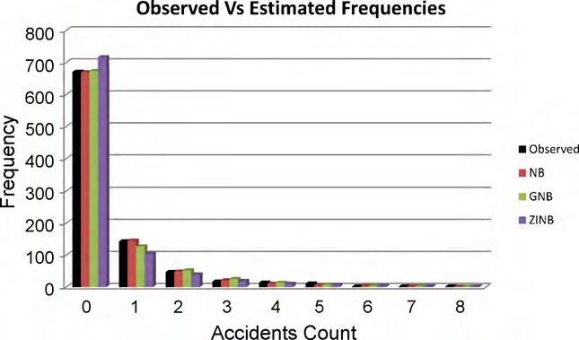
1880 T. Usman et al. / Accident Analysis and Prevention 42 (2010) 1878–1887
Fig. 1. Relation between maintenance, weather, traffic and safety.
3. Modeling of road surface conditions. ily represent the condition of the whole maintenance route. As a
4. Exploratory data analysis and development of statistical models. result, we did not use this data field directly and instead used it
to fill the missing RSC data from road condition weather informa-
3.1. Study sites tion system (RCWIS) and road weather information system (RWIS).
For this analysis only number of accidents and the time (hour)
For the proposed analysis, historical information on both road they occurred and road surface condition data, when no informa-
accidents and possible influencing factors must first be obtained. tion was available from RCWIS/RWIS data, are considered from this
This means that the sites that should be selected for this study must database.
be well instrumented so that detailed data on all major factors of
interest are available. In this research, after examining a number of
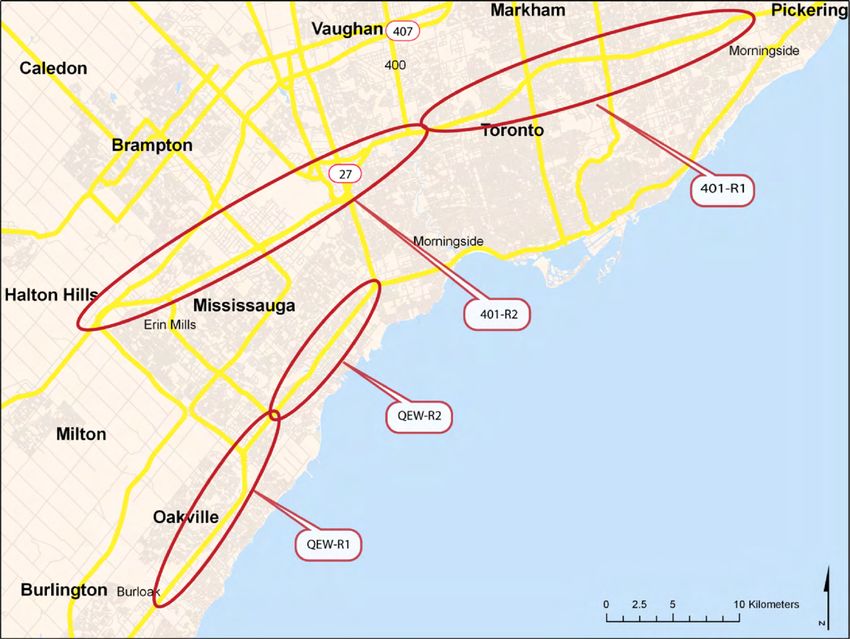
candidate sites, four patrol routes were selected. Two are on High- 3.1.3. Road condition weather information system (RCWIS) data
way 401 and two are on the Queen Elizabeth Way (QEW) in the This data contains information about road surface conditions,
province of Ontario, Canada, as shown in Fig. 2: maintenance, precipitation type, accumulation, visibility and tem-
perature. RCWIS data is collected by MTO maintenance personnel,
• 401-R1: Hwy 400 to Morningside Ave (28.0 km). who patrol the maintenance routes 3–4 times during a storm
• 401-R2: Trafalgar Road to Hwy 400 (31.1 km). event on the average. One of the most important pieces of
• QEW-R1: Burloak Drive to Erin mills parkway (17.4 km). information in this data source is a description of road surface
• QEW-R2: Erin mills parkway to Eastmall (13.1 km). conditions based on the MTO’s internal condition classification
system. A detailed description of this data field and its process-
For the proposed investigation, five types of data sources are ing for the subsequent modeling analysis is given later. This data
needed, including weather data, traffic data, accident data, road is also used by MTO in their traveler’s road information system;
surface condition data and winter operations data. These data usu- however, it is utilized here for the first time for research pur-
ally originate from different sources and are managed by different poses.
organizations, as described in the following section.
3.1.1. Traffic volume data 3.1.4. Road weather information system (RWIS) data
Traffic volume data was obtained from loop detectors collected This data source contains information about temperature, pre-
by the Ontario Ministry of Transportation (MTO). The data were cipitation type, visibility, wind speed, road surface conditions,
then processed in Excel and converted into hourly traffic volume etc., recorded by the RWIS stations near the selected mainte-
data. Note that loop detectors are a commonly used technology for nance routes. All data except hourly precipitation were available on
collecting traffic data such as volume, speed and density. This data hourly basis. Hourly precipitations from RWIS sensors were either
was screened for any outliers caused by detector malfunction. not available or not reliable. As a result, we derive this information
from the daily precipitation reported by Environment Canada (EC).
3.1.2. Traffic accident data Temperature and RSC data from RWIS were used to fill in the miss-
The Ontario Provincial Police (OPP) maintains a database of all ing data from RCWIS. For visibility and wind speed RWIS was used
of the collisions that have been reported on Ontario highways. as the primary source.
A database including all of the collision records for the study
routes was obtained from the MTO. The database includes detailed
information on each collision, including accident time, accident 3.1.5. Environment Canada (EC) data
location, accident type, impact type, severity level, vehicle infor- Weather data from Environment Canada includes temperature,
mation, driver information, etc. Note that the data on the accident precipitation type and intensity, visibility and wind speed. Except
occurrence time and location are needed for data aggregation over precipitation related information, all data from this data source
space (e.g., highway maintenance route) and time (e.g., by hour). were used as a secondary source for filling in the missing data from
The data item related to road surface conditions in the accident RCWIS/RWIS. EC is the only reliable data source for precipitation
data represent the conditions at the time and location associated type and intensity and it was therefore used as the primary source
with the observed collisions only. Therefore, they do not necessar- for these variables.T. Usman et al. / Accident Analysis and Prevention 42 (2010) 1878–1887 1881
Fig. 2. Site map showing the location of the selected patrol routes.
3.2. Data processing After all weather and road condition related data are converted
into the hourly format, they were fused into a single data set on
As described previously, there are five types of data available for the basis of date and time. When multiple data were available for
each selected study site. Once these data are obtained, they need a given field, priority was given to RCWIS and RWIS data over EC
to be pre-processed for merging and integration. data because these data sources are collected near the study sites
Accident data are available as event records and therefore need and therefore considered to be more representative. Missing RSC
to be aggregated into hourly records by totalling the accidents that data from RCWIS were retrieved from accident data or RWIS data.
have occurred within each hour of the day. Other attributes associ- It was also assumed that the RSC at the hour right after a mainte-
ated with accidents are averaged over each hour. The output of this nance treatment was done could be considered as partially snow
process is hourly data records of the total number of accidents and covered. This data field was then subsequently linearly interpo-
the associated average conditions such as speed, light, road surface lated for hourly conditions, as discussed in the following section.
conditions, precipitation, road physical characteristics, etc. This gave us values of road surface conditions for all hours over
The weather data is from three different sources, namely RCWIS, individual storms. In case of any missing data for temperature, pre-
RWIS and EC. RCWIS data, organized by patrol yards, are descriptive cipitation and wind in RCWIS, data from RWIS or EC data were used.
(or categorical) and non continuous in nature, similar to event- This process resulted in a single hourly based weather data set.
based records with a time stamp. As a result, two immediate issues Once the three sources of data were finalized, a single data set
need to be addressed. First, the original RCWIS data classify road was formed by combining all the data sets on the basis of date and
surface conditions (RSC) into a total of 160 classes, which make time.
it difficult to be directly modeled as a categorical factor in a sta-
tistical analysis. The second issue is that a large number of hours 3.3. Modeling of road surface conditions
do not have RSC observations. As a result, some assumptions have
to be introduced to interpolate the RSC between observations, as As described previously, MTO reports RSC using qualitative
detailed in the section. RWIS data are recorded every 20 min and descriptions, i.e., a categorical measure (e.g., 7 major categories
can be easily aggregated into hourly records based on their time and 160 subcategories). However, these categories have intrinsic
stamps. ordering in terms of the severity, which means that a more sensible
Hourly data from Environment Canada was obtained for type measure would be an ordinal one. While binary variables could be
of precipitation, visibility, wind speed, etc. However, precipita- used to code ordinal data, it would mean loss of information on the
tion intensity data are available only as a daily total, which is the ordering. We therefore decided to use an interval variable to map
water equivalent of the total precipitation amount over a day. Based the RSC categories and at the same time make sure that the new
on the data on “precipitation type” the hours with and without variable has physical interpretations. Road surface condition index
precipitation were decided. The total daily precipitation was then (RSI), a surrogate measure of the commonly used friction level, was
uniformly allocated to each hour of the hours with precipitation. therefore introduced to represent different RSC classes described in1882 T. Usman et al. / Accident Analysis and Prevention 42 (2010) 1878–1887
Fig. 3. RSI for different road surface classes.
RCWIS. The reason to use a friction surrogate is that there have been tify the individual events with the available hourly data records.
good amounts of field studies available on the relationship between For the purpose of this research, events are defined on the basis
descriptive road surface conditions and friction, which provided the of not only weather conditions but also of road surface conditions.
basis for us to determine boundary friction values for each category. This approach makes this research different from other event-based
To map the categorical RSC into RSI, the following procedure was studies where events are mostly defined based on environmental
used: data alone (e.g., Knapp et al., 2002).
Each event is defined with the following constraints:
(1) The major classes of road surface conditions, defined in RCWIS,
were first arranged according to their severity in an ascend- • An event starts at the time when snow/freezing rain is observed.
ing order as follows: Bare and Dry < Bare and Wet < Partly Snow • An event ends when snow/freezing rain stops and a certain pre-
Covered < Snow Covered < Snow Packed < Slushy < Icy. defined road surface condition is achieved after that time.
This order was also followed when sorting individual sub • Precipitation must be greater than zero (0).
categories in a major class. • Air temperature must be less than 5 ◦ C.
(2) Road surface condition index (RSI) was defined for each major • Road surface conditions index value must not be equal to bare
class of road surface state defined in the previous step as a dry conditions.
range of values based on the literature in road surface condition
discrimination using friction measurements (Wallman et al., This definition of storm events along with road weather, surface
1997; Wallman and Astrom, 2001; Transportation Association conditions and maintenance activities is schematically illustrated
of Canada, 2008; Feng et al., 2010). For convenience of inter- in Fig. 4. The numbers of snow storm events and accidents that were
pretation, RSI is assumed to be similar to road surface friction identified for individual routes are given in Table 1.
values and thus varies from 0.1 (poorest, e.g., ice covered) to 1.0
(best, e.g., bare and dry).
4. Model development
(3) Each category in the major classes is assigned a specific RSI
value. For this purpose, sub categories in each major category
In road safety literature, the most commonly employed
were sorted as per step 1 above. Linear interpolation was used
approach for modeling accident frequencies is the regression
to assign RSI values to the sub categories.
analysis for count data. In particular, the Negative Binomial (NB)
model and its extensions have been found to be the most suitable
RSI values for major road surface classes are given below:
distribution structures for road accident frequency (Shankar et
Road surface condition major classes RSI range al., 1995; Miaou and Lord, 2003; Miranda-Moreno, 2006; Sayed
Bare and dry 0.9–1.0 and El-Basyouny, 2006). Among the NB model extensions, we can
Bare and wet 0.8–0.89 mention the generalized NB, latent class NB and zero inflated NB
Partly snow covered 0.5–0.79
Snow covered 0.25–0.49
Snow packed 0.2–0.24 Table 1
Slushy 0.16–0.19 Number of events for each maintenance route.
Icy 0.1–0.15
Patrol no. Route length No. of No. of Accidents per
Fig. 3 shows variation of RSI for major categories. (km) events accidents event
401-R1 28 249 262 1.05
3.4. Generation of event-based dataset
401-R2 31.1 259 158 0.61
QEW-R1 17.4 204 34 0.17
After the hourly data set as prepared, an event-based data QEW-R2 13.1 200 32 0.16
set was generated by aggregating the hourly data over individual
Total – 912 486 0.53
events. An important step in this data aggregation step was to iden-T. Usman et al. / Accident Analysis and Prevention 42 (2010) 1878–1887 1883
Fig. 4. Road surface condition index variation over a snow storm event.
models — (for instance see Miaou, 1994; Shankar et al., 1997; • Total number of accidents over the event.
Miranda-Moreno, 2006). In this research, the NB model is there- • Event duration (h).
fore first evaluated for its performance in capturing observed and • Average visibility (km).
unobserved accident variations among individual snow storms. • Average air temperature (◦ C).
This model can be written as, Yi ∼ NB(i , ˛), where Yi represents • Average wind speed (km/h).
the number of accidents during an event i (i = 1, . . ., n), i stands • Precipitation type (1 = freezing rain, 2 = snow).
for the mean accident frequency, and ˛ is the over-dispersion • Total precipitation3 (mm).
parameter. Furthermore, it is assumed that the mean accident • Hourly precipitation (mm).
frequency (i ) is a function of a set of covariates through the log • Hourly traffic volume (vehicles/h).
link function commonly used in the road safety literature, that is: • Maintenance (1 = Sanding, 2 = Salting, 3 = Plowing, 4 = Sanding
and Salting, 5 = Sanding and Plowing, 6 = Salting and Plowing,
i = exp(ˇ0 + ˇ1 Ln(Exposure) + ˇ2 xi1 + ˇ3 xi2 + · · · + ˇk xik ) (1) 7 = Sanding and Salting and Plowing).
ˇ1
• Exposure (product of total traffic volume4 during the event and
i = (Exposure) exp(ˇ0 + ˇ2 xi1 + ˇ3 xi2 + · · · + ˇk xik ) (2)
segment length, converted into million vehicle kilometers or
where xij is the jth attribute associated with event i, Exposure MVkm).
• Average road surface conditions index (1 = bare pavement to
is as defined in Section 4.1 and (ˇ0 , ˇ1 , . . ., ˇk ) is a vector of
regression parameters. One of the shortcomings of the NB model 0.10 = icy pavement).
is the assumption of a constant over-dispersion parameter (˛) for
all observations. This assumption can be relaxed by assuming that Five sets of data were formed: one for each patrol route and
the dispersion parameter is a function of a set of covariates, using one including all patrol routes together. All the data sets were
an exponential link function as follows: checked for any outliers using box plots of individual data fields
in the database. A number of two way interactions were also con-
˛i = exp(0 + 1 zi1 + 2 zi2 + · · · + k zim ) (3) sidered for some of the variables. Note that these interaction terms
were identified on the basis of some possible physical interpreta-
where (zi1 , . . ., zim ) is a vector of event-specific factors that may tion; terms that are more complicated are not recommended to
be different than those explaining i and ( 0 , 1 , . . ., m ) is a include in regression models due to the added challenge of model
vector of parameters. The resulting model is commonly referred interpretation.
to as generalized Negative Binomial (GNB) model (Miaou and A correlation analysis was also carefully conducted for each
Lord, 2003; Miranda-Moreno et al., 2005; Miranda-Moreno, 2006). individual and combined dataset. As suspected, it was found that
This model may allow more flexibility than its alternatives to deal precipitation type and maintenance operations were consistently
with the well known over-dispersion problem and unobserved correlated with RSC across all datasets (with a correlation coeffi-
heterogeneities among events. cient greater than 0.60) and were therefore excluded from further
The third model considered in this research is called zero- analysis. Descriptive statistics are presented for variables found
inflated NB or ZINB model, which is also an extension of the significant in Table 2.
standard NB model. This assumes a dual state process in accident
occurrence: one generating safe events with zero accidents (Yi ∼ 0
5. Model calibration
with probability p) and the other state following an NB distribu-
tion [Yi ∼ NB(i , ˛) with probability 1 − p]. The ZINB model may
After the exploratory analysis, the next step is to specify the
be more flexible compared to the NB model since it can handle
functional form and to fit the model to the data. Because of the
both over-dispersion due to unobserved heterogeneity and excess
relatively small number of events per patrol and the large number
of zero counts. These three modeling options are all evaluated for
of independent variables that need to be evaluated for their effect
their suitability to fit the given data.
on accident frequency, the sample size for each individual site may
not be large enough for arriving at trustworthy results (Wright,
4.1. Exploratory data analysis
After the events were extracted from the hourly data records, the 3
Sum of precipitation for all the hours of an event.
following factors/variables were calculated for each storm event: 4
Sum of the hourly traffic volumes of an event.1884 T. Usman et al. / Accident Analysis and Prevention 42 (2010) 1878–1887
Table 2
Descriptive statistics.
Variables N Minimum Maximum Mean Std. deviation
Descriptive statistics – 401-R1
Visibility (km) 249 0.8 24.1 13.093 6.689
Road surface condition index 249 0.225 0.986 0.764 0.196
Accidents 249 0 19 1.050 2.123
Total precipitation (mm) 249 0.12 141.53 12.684 21.212
Ln(Exposure) 249 −2.656 3.256 0.303 1.161
Hourly traffic 249 1254 60197 11907 8684
Descriptive statistics – 401-R2
Visibility (km) 259 1.05 24.1 13.726 6.820
Road surface condition index 259 0.330 0.987 0.716 0.185
Accidents 259 0 8 0.610 1.167
Total precipitation (mm) 259 0.12 141.53 12.417 21.865
Ln(Exposure) 259 −2.812 3.581 0.354 1.292
Hourly traffic 259 966 60197 11101 8641
Descriptive statistics – QEW-R1
Visibility (km) 204 2.67 24.1 13.116 6.711
Road surface condition index 204 0.13 0.983 0.675 0.238
Accidents 204 0 5 0.167 0.589
Total precipitation (mm) 204 0.2 246 14.403 27.264
Ln(Exposure) 204 −2.938 3.006 0.583 1.053
Hourly traffic 204 1485 77330 25670 14090
Descriptive statistics – QEW-R2
Visibility (km) 200 1.8 24.1 12.923 6.319
Road surface condition index 200 0.13 0.98 0.660 0.244
Accidents 200 0 5 0.160 0.571
Total precipitation (mm) 200 0.2 246 15.101 27.763
Ln(Exposure) 200 −4.216 2.58 0.337 1.100
Hourly traffic 200 816 77330 25112 13970
Descriptive statistics – Patrol all
Visibility (km) 912 0.8 24.1 13.241 6.649
Road surface condition index 912 0.13 0.987 0.708 0.217
Accidents 912 0 19 0.533 1.378
Total precipitation (mm) 912 0.12 246 13.523 24.355
Ln(Exposure) 912 −4.22 3.58 0.388 1.167
Hourly traffic 912 816 77330 17652 13281
1995). As a result, in this research we focused only on the combined parable to GNB. Considering the small difference in LL and AIC
dataset assuming that the direction and magnitude of the effect between NB and GNB, NB might also be a model of choice based
of individual factors on accident frequency are consistent across on the principle of parsimony.
the four maintenance routes. A dummy variable characterizing the
patrol routes is included to capture the remaining effect caused 5.1. Model interpretation and application
by other route specific factors such as location, driver population,
and road geometry. A stepwise elimination process was followed In general, results from the three models are consistent, as
to identify the significant factors. STATA5 (Version 9) was used for shown in Table 3. Most results obtained in our research are con-
this analysis. sistent with those reported in the literature, with some exceptions.
Following the sequential regression process, we found that 4 of The following specific observations could be made from the mod-
11 factors were statistically significant at p < 0.05 for the three dif- eling outcome:
ferent model assumptions, including RSI, visibility, exposure and
site effect. As shown in Table 3, the calibration results are quite
• The most interesting result is perhaps that the RSI was found
consistent in terms of significant factors and coefficients across
to be a statistically significant factor influencing road safety
the models. After the three types of models were calibrated, the
across all sites. The negative sign associated to the factor sug-
best fit model was identified using log likelihood value and Akaike
Information Criterion (AIC) (Akaike, 1974). These test statistics are
widely used to identify the best fit model from a set of models.
The AIC statistic is defined as −2LL + 2p, where LL is the log likeli-
hood of a fitted model and p is the number of parameters, which is
included to penalize models with higher number of parameters: a
model with smaller AIC value represents a better overall fit. Based
on both the log likelihood value and AIC criterion, GNB was found
to be the best fitted model for the data (see Table 3).
In addition to using log likelihood values and AIC for best fit
model, we also compared the observed vs. the estimated relative
frequencies of the number of accidents (Maher and Summersgill,
1996; Miranda-Moreno, 2006). Fig. 5 shows this plot and from this
we can observe that all models fit well to the data and NB is com-
5
http://www.stata.com/. Fig. 5. Observed vs. estimated accident frequencies.T. Usman et al. / Accident Analysis and Prevention 42 (2010) 1878–1887 1885
Table 3
Summary results of model calibration.
Variable NB GNB ZINB
Coeff Sig Coeff Sig Coeff Sig
Intercept −0.400 0.174 −0.164 0.628 0.183 0.603
Visibility (km) −0.041 0.000 −0.041 0.000 −0.026 0.017
Road surface condition index −2.012 0.000 −2.276 0.000 −2.564 0.000
Ln(Exposure) 0.402 0.000 0.377 0.000 0.320 0.000
401-R1 1.986 0.000 2.034 0.000 1.879 0.000
401-R2 1.452 0.000 1.400 0.000 1.349 0.000
QEW-R1 −0.038 0.889 0.032 0.926 −0.031 0.910
QEW-R2 0.000 0.000 0.000
Number of observations 912 912 912
Log likelihood (constant only) −784.57 −903.07 −911.62
Log likelihood value at convergence −728.56 −718.06 −719.09
AIC 1473.12 1462.12 1462.18
Ln(Alpha) −0.014 −0.604
Intercept 2.134 0.001 2.736 0.002
Ln(Exposure) −0.329 0.017 −0.433 0.026
Hourly precipitation −0.357 0.025 −1.014 0.005
Hourly traffic
Road surface condition index −3.966 0.002
401-R1 −1.545 0.008
401-R2 −1.168 0.058
QEW-R1 0.634 0.351
QEW-R2 0.000
gests that higher accident frequencies associated with poor road however, one possible reason for this may be that Hwy 401 has
surface conditions. This result makes intuitive sense and has more interchanges per kilometer than QEW, which is known to
confirmed the findings of many past studies (Norrman et al., be an important factor influencing freeway safety in general.
2000; Wallman et al., 1997), mostly from Nordic countries. How- • Both air temperature and precipitation had a statistically insignif-
ever, this research is the first showing the empirical relationship icant effect on accident frequency. It was found that they are
between safety and road surface conditions at a disaggregate both partially correlated with RSC (0.26 for air temperature and
level, making it feasible to quantify the safety benefit of alter- −0.46 for precipitation). These results confirm some of the ear-
native maintenance goals and methods. lier findings (Hermans et al., 2006) but are in contradiction to
• Visibility is also found to have a statistically significant effect others (Andrey et al., 2001; Fu et al., 2006). Precipitation was also
on accident frequency during a snow storm. The negative model partially correlated with visibility (−0.38) (Andrey et al., 2001).
coefficient also makes intuitive sense, as it suggests that reduced Our result therefore makes intuitive sense as the effects of these
visibility was associated with increased number of accidents. two factors have already been accounted for through the RSC and
Note that this result is different from those from a past study by visibility factors.
Hermans et al. (2006), which conducted a statistical study using • In our analysis, we did not consider maintenance operations
data from 37 sites and found that visibility was significant only directly, which were assumed to be reflected in their end results,
at two sites. Their study however considered collisions occurring that is, road surface conditions. Our exploratory analysis also
at different roadways related to a single weather station. This found that maintenance was correlated with road surface con-
approach may have masked the effect of visibility due to con- ditions and were not statistically significant after road surface
founding of missing factors and large aggregation levels in both conditions were accounted for.
space (coastal areas vs. inter cities) and time (seasonal variation).
• As expected, exposure, defined as total vehicle kilometers trav- Because of the exponential functional form, the exponent in the
eled (product of the total traffic volume over a storm event and model is a measure of sensitivity of crash frequency to the corre-
route length), was found to be significant, suggesting that an sponding variable. For example, the coefficient associated with RSI
increase in traffic volume, storm duration, or route length would in the GNB is −2.276, which suggests that a 1% improvement in
lead to increase in number of accidents. Inclusion of this term RSI would lead to approximately a 2.28% reduction in the expected
ensures that traffic exposure is accounted for when estimating number of accidents.
the safety benefits of some specific policy alternatives. The coef- The calibrated model could be applied for assessing the safety
ficient associated with the exposure term has a value less than benefit of alternative winter road maintenance Level of Service
one (0.377), suggesting that the moderating effect of exposure is (LOS) goals for a specific maintenance route under a specific snow
non-linear with a decreasing rate. This result is consistent with storm event. Fig. 6 shows the relationship between the number of
those from road safety literature (e.g., Andrew and Bared, 1998; accidents that are expected to occur on the 28 km stretch of High-
Lord and Persaud, 2000; NCHRP Synthesis report No. 295, 2001; way 401 (401-R1 in Fig. 2) and the average road surface condition
Roozenburg and Turner, 2005; Mustakim et al., 2006; Sayed and over an assumed snow storm. Again, the GNB is chosen for this anal-
El-Basyouny, 2006; Sayed and Lovegrove, 2007; Jonsson et al., ysis. The assumed snow storm lasts for a total of 8 h with average
2007; Lord et al., 2008; etc.). visibility of 13 km. Three levels of traffic are considered, includ-
• The model also suggests that, controlling for other factors (RSC, ing 50,000, 100,000 and 150,000. The safety effect of maintaining
Visibility and Exposure), Hwy 401 (401-R1 and 401-R2) is more the road section at a given level of road surface condition over the
susceptible to crashes than the QEW (QEW-R1 and QEW-R2) event, as represented by RSI, can be estimated as the mean num-
while the difference in risk between the two maintenance routes ber of accidents corresponding to the RSI. For example, an average
on the same Highway is quite small. The exact reason for this dis- reduction of about three accidents could be achieved by maintain-
crepancy between 401 and QEW needs to be further investigated; ing the route at an RSI of 0.8 as compared to the snow packed icy1886 T. Usman et al. / Accident Analysis and Prevention 42 (2010) 1878–1887
road safety to some direct road surface condition measures. As part
of this work, three different regression models were developed and
evaluated using data from four instrumented freeway sections in
Ontario, Canada. From the calibrated models, interesting results
were obtained. For instance, the study has shown the statistically
significant link between road surface conditions represented by RSI
and road safety. As illustrated in the paper, this result gives the
opportunity to assess the safety benefit of alternative winter road
maintenance goals under different weather and traffic conditions.
This methodology can be applied to any other roadway sections
with detailed high-quality data on road weather conditions, traffic,
maintenance and accidents.
Our future efforts will concentrate on examining the validity of
these findings across a wider spectrum of weather, highway, traffic
and maintenance conditions, and exploring new model structures
Fig. 6. Accident frequency as a function of RSI. such as simultaneous equation models for addressing potential
endogeneity problems between traffic and accidents. This can be
caused by unobserved factors such as speed variations associated
scenario (RSI = 0.2) for traffic level of 100,000 vehicles. It can be seen with both traffic volumes and accidents. A modeling approach
from Fig. 6 that effects of traffic volume are more pronounced under accounting for potential correlation between events will be also
poor road surface conditions than good road surface conditions. For attempted. These models can help to improve the explanatory
instance, the expected number of accidents for an RSI value of 0.1 power of the models and the accuracy of the model parameters.
and high traffic is 5.2 accidents, while this value is 3.44 for a low
traffic scenario. This means that the difference between low and Acknowledgements
high traffic for RSI = 0.1 is 1.77 accidents. At the other extreme, for
an RSI value of 1.0, the difference between the low and high traffic This research was supported by MTO in part through the
condition is 0.23 accidents. Highway Infrastructure and Innovation Funding Program (HIIFP).
To show further applications of the developed model, we apply The first author also wishes to thank Higher Education Commis-
the model for two hypothetical case studies. The first case study is sion, Pakistan for their financial support. The authors wish to
to assess the safety implication of adopting different bare pavement acknowledge in particular the assistance of Max Perchanok, Steve
(BP) recovery time, one of the critical policy variables in winter road Birmingham, Zoe Lam and David Tsui from MTO and Brian Mills
maintenance operations. The same example described previously from Environment Canada.
is used with a traffic flow rate of 12,500 vehicles per hour. The
snow event is assumed to last 8 h: 4 h of precipitation and 4 h of BP References
recovery time.
In the first case, it is assumed that little maintenance work Akaike, H., 1974. A new look at the statistical model of identification. IEEE Transac-
tion on Automatic Control 19, 716–723.
such as salting was done and the road surface was deteriorated Andreescu, M.P., Frost, D.B., 1998. Weather and traffic accidents in Montreal, Canada.
from bare dry to bare wet passing through snow covered condi- Climate Research 9, 225–230.
tions. Two road surface conditions are considered, namely, snow Vogt, A., Bared, J., 1998. Accident models for two-lane rural segments and intersec-
tions. Transportation Research Record 1635. Paper No. 98-0294.
covered and bare pavement. For snow covered conditions, the cor- Andrey, J., Mills, B., Vandermolen, J., 2001. Weather Information and Road Safety.
responding RSI is assumed to be 0.2 (average condition within the Institute for Catastrophic Loss Reduction, Toronto, Ontario, Canada.
snow storm) while the bare pavement surface is assumed to have Buchanan, F., Gwartz, S.E., 2005. Road weather information systems at the Ministry
of Transportation, Ontario. In: Presented at Annual Conference of the Trans-
a RSI of 0.8. It is also assumed that before the start of the storm
portation Association of Canada Calgary, Alberta.
road surface is dry with a RSI of 1.0. For this scenario, the aver- Eisenberg, D., Warner, K.E., 2005. Effects of snowfalls on motor vehicle colli-
age RSI = (1.0 + 7.0 × 0.2 + 0.8)/9 = 0.356. Mean number of accidents sions, injuries, and fatalities. American Journal of Public Health 95 (1), 120
(ABI/INFORM Global).
in this case are 2.50.
Environment Canada, 2002. Winter road maintenance activities and the use of road
Now, we consider the alternative scenario of reducing the BP salts in Canada: a compendium of costs and benefits indicators.
recovery time to 3 h. This means reducing the storm duration to 7 h Feng, F., Fu, L., Perchanok, M.S., 2010. Comparison of alternative models for road
(4 h of precipitation and 3 h of BP recovery time). Under the same surface condition classification. TRB Annual Meeting 2010. Paper #10-2789.
Fu, L., Perchanok, M.S., Moreno, L.F.M., Shah, Q.A., 2006. Effects of winter weather and
conditions, the new average RSI = (1.0 + 6 × 0.2 + 0.8)/8 = 0.375. maintenance treatments on highway safety. TRB 2006 Annual Meeting. Paper
Mean number of accidents in this case are 2.27, that is, a 9% reduc- No. 06 – 0728.
tion. Hanbali, R.M., Kuemmel, D.A., 1992. Traffic accident analysis of ice control
operation. http://www.trc.marquette.edu/publications/IceControl/ice-control-
In second case it is assumed that some other maintenance work 1992.pdf (accessed March 03, 2009).
such as plowing has been done in the second hour raising RSI Handman, A.L., 2002. Weather implications for urban and rural public transit.
to 0.8 then dropping in a linear way to 0.4 at the end of fourth http://ams.confex.com/ams/pdfpapers/74636.pdf (accessed June 26, 2007).
Hermans, E., Brijis, T., Stiers, T., Offermans, C., 2006. The impact of weather conditions
hour due to precipitation and remain so till the seventh hour after on road safety investigated on an hourly basis. TRB Annual Meeting 2006. Paper
which it raises back to RSI = 0.8. For this case the new average No. 06-1120.
RSI = (1.0 + 2 × 0.2 + 2 × 0.8 + 0.6 + 4 × 0.4)/10 = 0.520. Mean number Jonsson, T., Ivan, J.N., Zhang, C., 2007. Crash prediction models for intersections on
rural multilane highways – differences by collision type. TRR Journal (2019),
of accidents in this case are 1.72. The relative reduction in the mean
91–98, doi:10.3141/2019-12.
number of accidents is therefore 31.2%. Knapp, K.K., Smithson, D.L., Khattak, A.J., 2002. The mobility and safety
impacts of winter storm events in a freeway environment. http://www.ctre.
iastate.edu/pubs/midcon/knapp1.pdf (accessed December 01, 2007).
6. Conclusions and future work Kumar, M., Wang, S., 2006. Impacts of weather on rural highway Opera-
tions Showcase Evaluation # 2. http://www.coe.montana.edu/wti/wti/pdf/
This paper has presented the results of a modeling approach 426243 Final Report.pdf (accessed June 26, 2007).
Lord, D., Persaud, B.N., 2000. Accident prediction models with and without trend:
aimed at explaining the variation of road accidents over different application of the generalized estimating equations (GEE) procedure. TRB 79th
snow storm events. This approach allows for the relation of winter Annual Meeting. Paper No. 00-0496.T. Usman et al. / Accident Analysis and Prevention 42 (2010) 1878–1887 1887
Lord, D., Guikema, S.D., Geedipally, S., 2008. Application of the Roskam, A.J., Brookhuis, K.A., Waard, D.d., Carsten, O.M.J., Read, L., Jamson, S.,
Conway–Maxwell–Poisson generalized linear model for analyzing motor Ostlund, J., Bolling, A., Nilsson, L., Antilla, V., Hoedemaeker, M., Janssen, W.H.,
vehicle crashes. Accident Analysis and Prevention 40 (3), 1123–1134. Harbluk, J., Johansson, E., Tevell, M., Santos, J., Fowkes, M., Engstrom, J., Vic-
Maher, M.J., Summersgill, I., 1996. A comprehensive methodology for the fitting tor, T., 2002. Human machine interface and safety of traffic in Europe. Project
predictive accident models. Accident Analysis and Prevention 28 (3), 281–296. GRD1/2000/25361 S12.319626.
Miaou, S.P., 1994. The relationship between truck accidents and geometric design of Sayed, T., El-Basyouny, K., 2006. Comparison of two negative binomial regression
road sections: Poisson versus negative binomial regressions. Accident Analysis techniques in developing accident prediction models. TRR Journal (1950), 9–
and Prevention 26, 471–482. 16.
Miaou, S.P., Lord, D., 2003. Modeling traffic crash–flow relationships for intersec- Sayed, T., Lovegrove, G.R., 2007. Macrolevel collision prediction models to enhance
tions: dispersion parameter, functional form, and Bayes versus empirical Bayes. traditional reactive road safety improvement programs. TRR Journal (2019),
TRR Journal 1840, 31–40. 65–73, doi:10.3141/2019-09.
Miranda-Moreno, L.F., Fu, L., Saccomano, F., Labbe, A., 2005. Alternative risk models Shankar, V., Mannering, F., Barfield, W., 1995. Effect of roadway geometrics and
for ranking locations for safety improvement. TRR Journal 1908, 1–8. environmental factors on rural freeway accident frequencies. Accident Analysis
Miranda-Moreno, L.F., 2006. Statistical models and methods for identifying haz- and Prevention 27 (3), 371–389.
ardous locations for safety improvements. PhD thesis report, University of Shankar, V., Milton, J., Mannering, F., 1997. Modeling accident frequencies as
Waterloo. zero-altered probability processes: an empirical inquiry. Accident Analysis and
Mustakim, F.B., Daniel, B.D., Bin, K., 2006. Accident investigation, blackspot treat- Prevention 29 (6), 829–837.
ment and accident prediction model at federal route FT50 Batu Pahat-Ayer Transport Canada. Canadian Environmental Protection Act, 1999. Priority substances
Hitam. Journal of Engineering e-Transaction vol. 1, no. 2, pp. 19–32, University list assessment report, road salts.
of Malaya. Transport Association of Canada, 2003. Salt smart train, the trainer program. Salt
National Cooperative Highway Research Program, Synthesis 295, 2001. Statistical smart learning guide.
Methods in Highway Safety Analysis, A Synthesis of Highway Practice. TRB Transportation Association of Canada, 2008. Winter maintenance performance mea-
Executive Committee. surement using friction testing. Final draft report, September 2008.
Nixon, W.A., Qiu, L., 2008. Effects of adverse weather on traffic crashes: systematic Velavan, K., 2006. Developing tools and data model for managing and analyzing traf-
review and meta-analysis. TRB 87th Annual Meeting 2008. Paper No. 08 – 2320. fic accident. MSc thesis report. University of Texas at Dallas, School of Economic,
Norrman, J., Eriksson, M., Lindqvist, S., 2000. Relationships between road slip- Political and Policy Sciences for Master of Science in Geographic Information
periness, traffic accident risk and winter road maintenance activity. Climate Sciences.
Research 15, 185–193 (published September 05). Wallman, C.G., Wretling, P., Oberg, G., 1997. Effects of winter road maintenance. VTI
Perchanok, M.S., Manning, D.G., Armstrong, J.J., 1991. Highway Deicers: Standards, rapport 423A.
Practice, and Research in the Province of Ontario. Ministry of Transportation Wallman, C.G., Astrom, H., 2001. Friction measurement methods and the correla-
Ontario. tion between road friction and traffic safety – a literature review. VTI report
Qin, X., Noyce, D.A., Martin, Z., Khan, G., 2007. Road weather safety audit program M911A.
development and initial implementation. TRB 2007 Annual Meeting. Paper No. Wright, R.E., 1995. Logistic regression. In: Grimm, L.G., Yarnold, P.R. (Eds.), Reading
07 – 2684. and Understanding Multivariate Statistics. American Psychological Association,
Roozenburg, A., Turner, S., 2005. Accident prediction models for signalised intersec- Washington, DC, pp. 217–244.
tions. www.ipenz.org.nz/ipenztg/ipenztg cd/cd/2005 pdf/03 Roozenburg.pdf
(accessed June 2008).You can also read