Seismological Observations of Ocean Swells Induced by Typhoon Megi Using Dispersive Microseisms Recorded in Coastal Areas
←
→
Page content transcription
If your browser does not render page correctly, please read the page content below
remote sensing
Article
Seismological Observations of Ocean Swells Induced
by Typhoon Megi Using Dispersive Microseisms
Recorded in Coastal Areas
Jianmin Lin 1,2, * , Sunke Fang 1 , Xiaofeng Li 3 , Renhao Wu 1           and Hong Zheng 1, *
 1   Marine Acoustics and Remote Sensing Laboratory, Zhejiang Ocean University, Zhoushan 316021, China;
     fangsunke@outlook.com (S.F.); mikewu@zjou.edu.cn (R.W.)
 2   State Key Laboratory of Acoustics, Institute of Acoustics, Chinese Academy of Sciences,
     Beijing 100190, China
 3   Global Science and Technology, National Oceanic and Atmospheric Administration (NOAA)-National
     Environmental Satellite, Data, and Information Service (NESDIS), College Park, MD 20740, USA;
     xiaofeng.li@noaa.gov
 *   Correspondence: jmlin007@zjou.edu.cn (J.L.); seahzheng@msn.com (H.Z.);
     Tel.: +86-580-218-3617 (J.L.); +86-580-255-0753 (H.Z.)

 Received: 14 August 2018; Accepted: 6 September 2018; Published: 8 September 2018

 Abstract: Typhoons in the western Pacific Ocean can generate extensive ocean swells, some of which
 propagate toward Taiwan, Luzon, and the Ryukyu Islands, impacting the coasts and generating
 double-frequency (DF) microseisms. The dispersion characteristics of DF microseisms relevant to
 the propagation of ocean swells were analyzed using the fractional Fourier transform (FrFT) to
 obtain the propagation distance and track the origins of typhoon-induced swells through seismic
 observations. For the super typhoon Megi in 2010, the origin of the induced ocean swells was tracked
 and localized accurately using seismic records from stations in eastern Taiwan. The localized source
 regions and calculated wave periods of the ocean swells are in good agreement with values predicted
 by ERA5 reanalysis from the European Centre for Medium-Range Weather Forecasts (ECMWF).
 However, localized deviations may depend on the effective detection of dispersive DF microseisms,
 which is tied to both coastline geometry and the geographic locations of seismic stations. This work
 demonstrates the effectiveness of seismological methods in observing typhoon-induced swells. The
 dispersion characteristics of DF microseisms recorded by coastal stations could be used as a proxy
 measure to track and monitor typhoon-induced swells across oceans.

 Keywords: typhoon; ocean swell; microseism; seismic station

1. Introduction
     Swells induced by a typhoon can be devastating and commonly cause major damage to ships
and coastal infrastructure, as they can propagate over long distances with their energy only weakly
attenuated [1,2]. In addition to strong societal and environmental consequences, swells can have
observable impacts on ocean surface roughness, wind stress, air–sea interactions, global climate, and
possibly mixing in the global ocean [3–7]. As a result, research on swells recently became a subject
of increasing interest in the discipline of ocean science [8,9]. However, there is still little quantitative
research on this topic, and the processes that control swell evolution on large scales remain unclear.
     Based on the coherent persistence of swells along their propagation routes, synthetic aperture
radar (SAR) was shown to be an effective approach to track swells across the ocean [10–12].
Jiang et al. [13] successfully tracked the propagation of storm swells from source regions around
58◦ S, 132◦ W to the coast of Mexico using SAR wave mode data. Ardhuin et al. [2] observed the

Remote Sens. 2018, 10, 1437; doi:10.3390/rs10091437                     www.mdpi.com/journal/remotesensing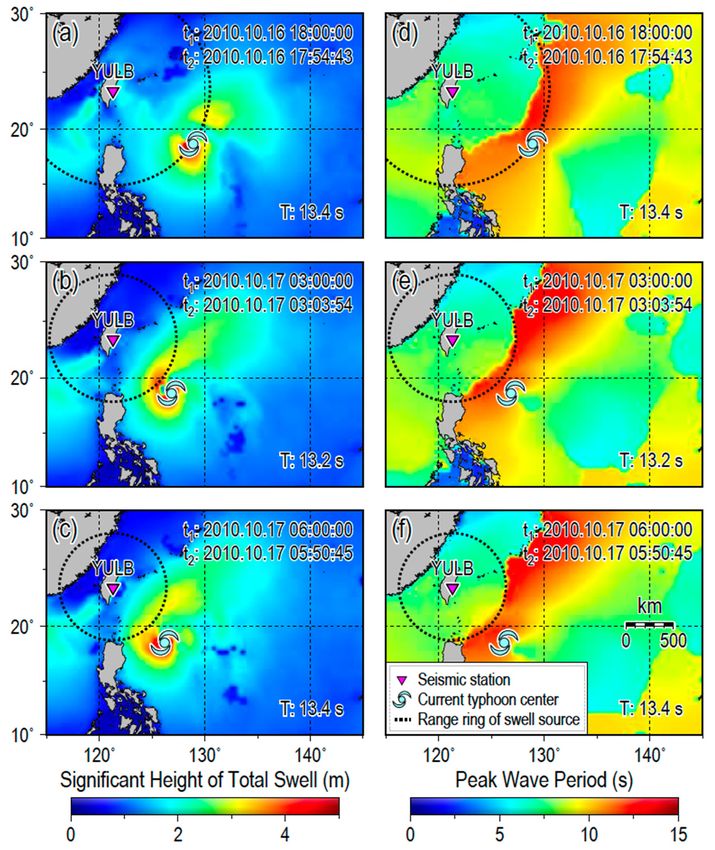
Remote Sens. 2018, 10, 1437                                                                     2 of 15

dissipation of swell energy from a number of storms using high-quality global SAR data, and found
that swells propagated distances of 2800 to >20,000 km, depending on the swell steepness. However,
SAR sampling cannot be applied when mismatched to the natural swell propagation. Consequently,
Ardhuin et al. obtained only 22 total estimates of the swell energy budget at peak periods of 13–18 s
from 10 storms recorded during the period 2003–2007.
     Because typhoon-induced swells seldom propagate across any measurement array that is
deployed in advance, it can be difficult to observe them using in situ measurements. To date, to
our knowledge, only the experiment of Snodgrass et al. [1] and the measurements of wind-wave
growth and swell decay during the Joint North Sea Wave Project (JONSWAP) by Hasselmann et al. [14]
were able to investigate swell evolution at large scales. Therefore, observational studies of swell
propagation are relatively scarce.
     In recent years, a new method of observing swells emerged, based on seismic records of
typhoon-generated noise (i.e., “microseisms”) [15–20]. Seismic noise is used here as a proxy for
swell monitoring in areas where ocean wave gauges are poorly instrumented. This interdisciplinary
approach, spanning ocean acoustics, marine geophysics, and physical oceanography, could also
remotely sense the propagation of swells generated by typhoons, with a focus on locating the source
area and estimating the origin times of swells. This is expected to complement existing observational
methods and numerical simulations of swells.
     Microseisms are the most energetic component of seismic noise, with a typical frequency peak of
~0.05–0.4 Hz [21–23]. Ocean wave activity was long accepted as the major source of microseisms [24].
A portion of the energy inherited from ocean waves at the sea surface (e.g., generated by typhoons)
can propagate to the sea floor or shoreline and be transferred to seismic waves in basement rocks
as microseisms. These microseisms can propagate as both surface waves (mainly Rayleigh) and
compressional (P) waves, which can be recorded by broadband seismometers located thousands of
kilometers from the source [25–28]. Recent studies also reported Love waves and S waves detected in
microseismic signals [29,30].
     Microseisms can be divided into two distinct bands in the frequency domain, which are
called single-frequency (SF, ~0.05–0.12 Hz) and double-frequency (DF, ~0.12–0.4 Hz) microseisms.
Each band is generated by a different physical process. SF microseisms are generated by the direct
interaction of pressure fluctuations induced by ocean waves with the shallow seafloor or the shore,
and therefore, typically have energy concentrated in the same frequency band as ocean waves [31].
Because ocean-wave-induced pressure fluctuations attenuate exponentially with water depth with
an e-folding constant equal to the wavenumber [32], the source regions of SF microseisms are
generally areas of shallow coastal water. DF microseisms are observed at higher intensities than SF
microseisms and are characterized by dominant frequencies of approximately twice the corresponding
ocean wave frequencies. They are generated by depth-independent seafloor pressure fluctuations
that are induced by the nonlinear interference of ocean waves with nearly opposite propagation
directions at similar periods [24]. Based on the Longuet-Higgins theory, Ardhuin et al. [33] developed
the first numerical model of DF microseism generation by random ocean waves and presented a
classification system for DF microseism generation from wave–wave interactions under typhoon
conditions. In their classification, Class-I microseisms are produced by interactions between opposing
ocean waves generated by a rapidly moving typhoon at different times, Class-II microseisms are caused
by the interaction between typhoon-induced swells incident on coasts and their coastal reflections, and
Class-III microseisms arise from interactions between ocean waves generated by two distinct typhoons.
     DF microseisms could be used to monitor typhoons and to track typhoon-induced
swells [25,28,34–36], because typhoon-induced swells are dispersive surface gravity waves that
propagate in deep water over long distances. The swells can reach and impact coastlines, generating
dispersive DF microseisms due to interactions between incident swells and opposing components
from coastal reflection. Consequently, the time–frequency evolution of dispersive DF microseisms is
closely related to the dispersion of typhoon-induced swells, and can, therefore, provide a potential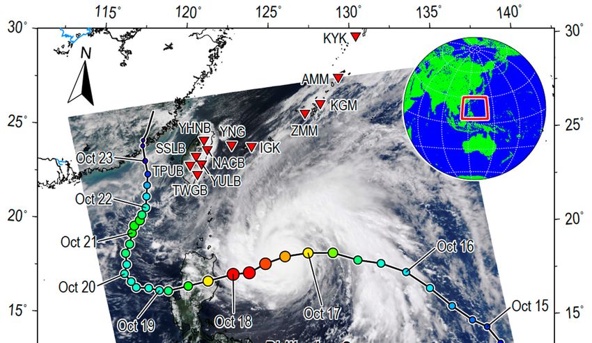
Remote Sens. 2018, 10, 1437                                                                         3 of 15

way to characterize the propagation of typhoon-induced swells, which are rarely observed using
conventional equipment.
      To our knowledge, Barruol et al. [17,18], Cathles et al. [19], and Davy et al. [20] are the only
existing studies that used seismic signals to remotely detect typhoon-induced ocean swells. Specifically,
Barruol et al. [17,18] used seismic stations as alternatives to ocean wave buoys for analyzing ocean
wave activity, employing microseisms to estimate swell height and propagation direction through
polarization analysis. Cathles et al. [19] used seismic observations of 93 distant ocean swell events
recorded on the Ross Ice Shelf during 2004–2006 to demonstrate that typhoon-induced swells could
have a tangible mechanical influence on the calving margins of the Antarctic Ice Sheet. Davy et al. [20]
investigated microseisms of extreme swell events recorded on La Réunion island using seismic
stations as ocean wave gauges, verifying that microseisms can provide valuable insights into extreme
swell events. Although both Barruol et al. [17,18] and Davy et al. [20] proposed retrieving the swell
propagation direction from the azimuth of the seismic noise using polarization analysis, these studies
treated the origin of each swell as a static point, rather than a dynamic feature with a distributed source
whose centroid changes with the temporal evolution of a typhoon.
      Approximately 30% of tropical cyclones occur in the northwest Pacific, which makes this an
ideal study area [37,38]. Typhoon Megi was one of the most intense typhoons in the northwest Pacific
during 2010, with Category 5 strength on the Saffir–Simpson hurricane wind scale. The present work
is a proof-of-concept study for investigations of typhoon-induced ocean swell origins during the
lifespan of Typhoon Megi, using seismic data recorded in coastal areas. We first investigated the DF
microseisms recorded during Typhoon Megi by terrestrial seismic stations on Taiwan and the Ryukyu
Islands. We then inverted for the origin time and source region of typhoon-induced swells using the
dispersion characteristics of DF microseisms, and obtained results that are generally consistent with
ERA5 reanalysis of ocean wave data. This demonstrates that seismic monitoring could allow us to
track typhoon-induced swells using microseisms recorded at coastal sites.

2. Data
     According to the best-track data of the Regional Specialized Meteorological Center (RSMC),
Megi formed over the deep Philippine Sea on 13 October 2010, and intensified to super typhoon
classification, with 10-min maximum sustained wind speeds up to ~230 km/h recorded early on
18 October 2010. Megi moved into the South China Sea (SCS), then turned north to the Taiwan Strait
after making landfall on Luzon Island, Philippines on 18 October 2010, and made a second and final
landfall in southeast (SE) China on 23 October (Figure 1). The long track course of Megi, with a
principally westward-moving direction over the deep Philippine Sea, provided ample opportunity to
generate intense ocean swells propagating toward Taiwan and the Ryukyu Islands. The subsequent
DF microseisms were used here to track typhoon-induced swells using seismological methods.
     Continuous vertical-component seismic waveform data recorded by stations in Taiwan and the
Ryukyu Islands were obtained from the Incorporated Research Institutions for Seismology (IRIS)
Data Management Center and the F-net network of Japan (Figure 1). The ERA5-reanalyzed ocean
wave data used in this paper were provided by the ECMWF. Downloaded data covered the period of
10–23 October 2010, comprising the lifespan of Typhoon Megi and three days prior to its onset.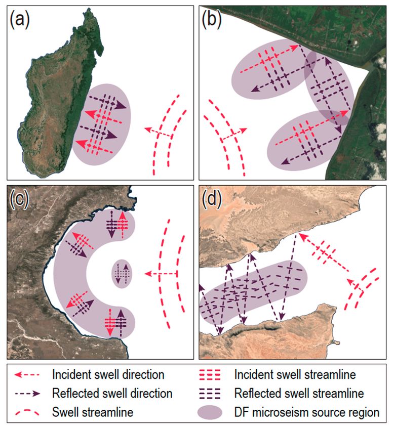
Remote Sens. 2018, 10, 1437 4 of 15
Remote Sens. 2018, 10, x FOR PEER REVIEW 4 of 15
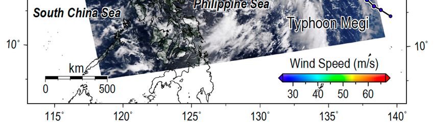
Figure 1.1. Distribution
Distributionofofseismic
seismicstations (red
stations triangles)
(red and and
triangles) trajectory of Typhoon
trajectory Megi (colored
of Typhoon circles)
Megi (colored
in the western
circles) Pacific Ocean,
in the western Pacificwith a superimposed
Ocean, Quick-Look
with a superimposed image of Megi
Quick-Look imagecaptured
of Megi by Modis by
captured on
17 Octoberon
Modis 2010 at
1704:55October
coordinated universal
2010 at time (UTC)coordinated
04:55 (https://ladsweb.modaps.eosdis.nasa.gov).
universal time (UTC)
The seismic stations are mostly from the Broadband
(https://ladsweb.modaps.eosdis.nasa.gov). The seismicArray in Taiwan
stations are for Seismology
mostly from the(BATS) and the
Broadband
F-net network
Array in Taiwan of Japan. The typhoon
for Seismology trackand
(BATS) is indicated
the F-netby roundedofcircles,
network Japan.equally spaced track
The typhoon in timeis
at six-hourbyintervals,
indicated rounded with circle
circles, size and
equally color
spaced in related
time at to wind speed.
six-hour Thewith
intervals, best-track dataand
circle size of Megi
color
were provided
related to wind byspeed.
the Japan
TheMeteorological Agency
best-track data of Megi(http://www.jma.go.jp/jma/jma-eng/jma-center/
were provided by the Japan Meteorological
rsmc-hp-pub-eg/trackarchives.html).
Agency (http://www.jma.go.jp/jma/jma-eng/jma-center/rsmc-hp-pub-eg/trackarchives.html).
To investigate
Continuous the characteristics
vertical-component of thewaveform
seismic microseisms datagenerated
recorded by bystations
typhoon-induced
in Taiwan and swells,
the
power
Ryukyuspectrograms
Islands werewere computed
obtained from the from seismic dataResearch
Incorporated to revealInstitutions
the intensity forofSeismology
the microseisms
(IRIS)
as a function
Data Managementof time and frequency.
Center Firstly,
and the F-net the original
network seismic
of Japan (Figurewaveform data were preprocessed
1). The ERA5-reanalyzed ocean
with the following steps: (1) demeaning and detrending;
wave data used in this paper were provided by the ECMWF. Downloaded data (2) removal of the instrument
covered the response;
period
(3) resampling
of 10–23 Octoberto 2010,
one point per second;
comprising and (4)of
the lifespan filtering
Typhoon withMegia band-pass
and threefilter
daysfrom
prior0.05
to itstoonset.
0.45 Hz.
Secondly, spectrograms were calculated from preprocessed data using a
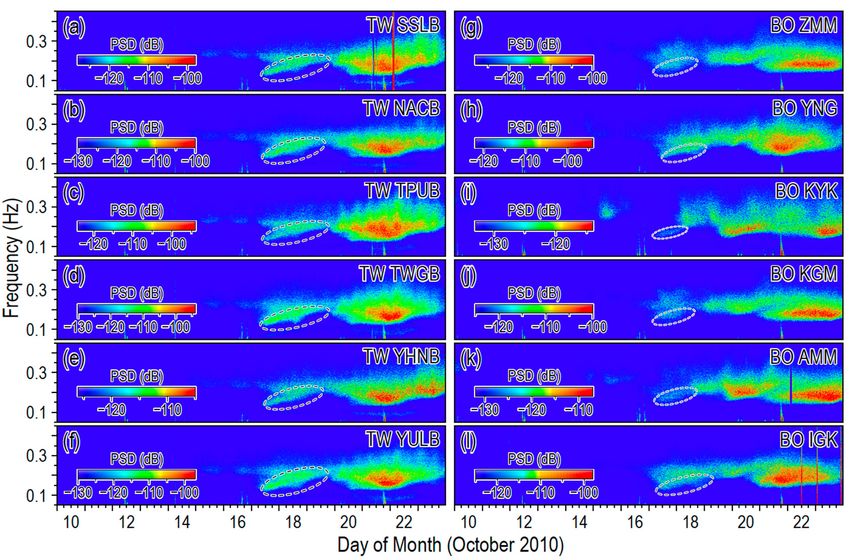
To investigate the characteristics of the microseisms generated by typhoon-induced swells,Fourier transform with a
power spectrograms were computed from seismic data to reveal the intensity of the microseisms as a2
moving-window length of 2048 samples shifted in steps of 1800 samples (i.e., half an hour). Figure
shows sample
function of timepower spectrograms
and frequency. recorded
Firstly, duringseismic
the original Typhoon Megi at the
waveform dataseismic stations indicated
were preprocessed with
by red triangles in Figure 1. The spectrograms effectively detected the
the following steps: (1) demeaning and detrending; (2) removal of the instrument response;DF microseisms generated (3) by
Megi, and were
resampling uncontaminated
to one by transient
point per second; and (4) events
filtering such as aearthquakes,
with instrumental
band-pass filter from 0.05 irregularities,
to 0.45 Hz.
and non-stationary noise, which appear as short pulses later in the spectrograms.
Secondly, spectrograms were calculated from preprocessed data using a Fourier transform The plots show the
with a
temporal evolution of recorded microseisms during the course of Megi. The dispersive
moving-window length of 2048 samples shifted in steps of 1800 samples (i.e., half an hour). Figure 2 DF microseismic
signalssample
shows inspiredpower
the investigation
spectrograms of the generation
recorded during and propagation
Typhoon Megiof attyphoon-induced
the seismic stations swells using
indicated
seismological observations.
by red triangles in Figure 1. The spectrograms effectively detected the DF microseisms generated by
Megi, and were uncontaminated by transient events such as earthquakes, instrumental
irregularities, and non-stationary noise, which appear as short pulses later in the spectrograms. The
plots show the temporal evolution of recorded microseisms during the course of Megi. The
dispersive DF microseismic signals inspired the investigation of the generation and propagation of
typhoon-induced swells using seismological observations.
Remote Sens. 2018, 10, 1437                                                                                            5 of 15
   Remote Sens. 2018, 10, x FOR PEER REVIEW                                                                           5 of 15

     Figure
       Figure2.2.Spectrograms
                    Spectrograms of of
                                     microseisms
                                       microseisms  from
                                                       fromTyphoon
                                                             Typhoon  Megi
                                                                        Megi recorded
                                                                               recordedbybyseismic
                                                                                             seismicstations
                                                                                                       stations(vertical
                                                                                                                 (vertical
     component)
       component)onon(a–f)(a–f)Taiwan
                                Taiwanand and(g–l)
                                                (g–l)the
                                                       theRyukyu
                                                           RyukyuIslands.
                                                                     Islands.TheThedashed
                                                                                      dashedellipses
                                                                                              ellipsesoutline
                                                                                                        outlineClass-II
                                                                                                                  Class-II
     (dispersive    double-frequency   (DF))  microseisms    generated    in coastal regions. Color
       (dispersive double-frequency (DF)) microseisms generated in coastal regions. Color scales varyscales  vary  from
                                                                                                                     from
     plot
       plottotoplot
                plotto
                     to emphasize the
                                   thedispersive
                                        dispersivecharacteristics
                                                      characteristics
                                                                    of of
                                                                       thethe
                                                                           DFDF   microseisms
                                                                               microseisms       at each
                                                                                            at each       station.
                                                                                                    station.        The
                                                                                                              The scaling
                                       log10
                                           10 ∙m
                                                 2 /Hzm. /Hz .
                                               log

     scaling   unitcorresponds
       unit (dB)                to 10· to
                    (dB) corresponds

3.3. Methods
  Methods
       Ouroverarching
     Our     overarchinggoal
                           goalwas
                                wastotoremotely
                                          remotelysense
                                                     sensethethegeneration
                                                                 generationofoftyphoon-induced
                                                                                  typhoon-inducedswells swellsvia
                                                                                                                via
  dispersive
dispersive   DFDFmicroseisms.
                  microseisms. ToTothat
                                     thatend,
                                          end,wewefirstly
                                                    firstlydetected
                                                            detectedthe
                                                                      thearrivals
                                                                          arrivalsofoftyphoon-induced
                                                                                        typhoon-inducedswells
                                                                                                            swells
  using the  principal function of  the spectrograms    calculated  before analysis.   We  then  identified
using the principal function of the spectrograms calculated before analysis. We then identified the         the DF
  (Class-II) microseisms  using the  swaths  of relatively  high signal energy  density   that tilt
DF (Class-II) microseisms using the swaths of relatively high signal energy density that tilt from  from lower-left
  to upper-right
lower-left        (indicating
            to upper-right    dispersion)
                           (indicating      in Figurein
                                         dispersion)   2 (dashed
                                                         Figure 2 ellipses).
                                                                   (dashed ellipses).
  3.1. Location and Timing of Swell Origin
3.1. Location and Timing of Swell Origin
        We calculated great-circle distances and travel times of typhoon-induced swell propagation from
      We calculated great-circle distances and travel times of typhoon-induced swell propagation
  the origin to the coastlines, where coastal seismic stations are deployed in the vicinity, based on the
from the origin to the coastlines, where coastal seismic stations are deployed in the vicinity, based on
  method presented by Munk et al. [39].
the method presented by Munk et al. [39].
        Typhoon-induced swells propagating on deep water could be considered as surface gravity waves.
      Typhoon-induced swells propagating on deep water could be considered as surface gravity
  According to the linear theory for waves forced by gravity, the group velocity could be expressed by
waves. According to the linear theory for waves forced by gravity, the group velocity could be
expressed by                                          r
                                                    1 gλ         g
                                              Cg =            =    T,                                    (1)
                                                    2 2π        4π
                                                  1 gλ         g
                                             Cg =           =     T,                                 (1)
  where g = 9.81 m · s−2 is acceleration due          2π λ 4isπwavelength, and T is wave period. Therefore,
                                                to2gravity,
  the group velocity increases with the period in deep water. Assuming ocean swells with frequency f w
where    g = 9.81
  propagate         m ⋅s−2x, is
              a distance     theacceleration duetravel
                                 corresponding    to gravity,   λ is wavelength,
                                                       time t could   be computedand   T is wave period.
                                                                                  as follows:
Therefore, the group velocity increases with the period in deep water. Assuming ocean swells with
                                                x    4πx
frequency f w propagate a distance x , the                f w . travel time t could be computed as(2)
                                           t =corresponding
                                                  =
                                               Cg      g
follows: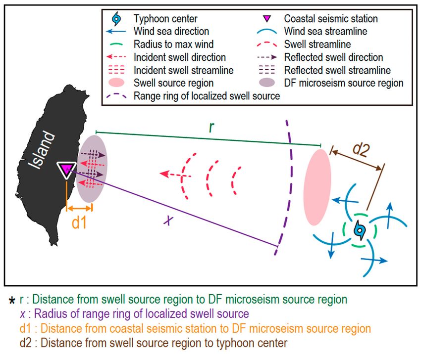
Remote Sens. 2018, 10, 1437                                                                        6 of 15

      The partial derivative from Equation (2) is

                                               dt    4πx
                                                   =     .                                             (3)
                                              d fw    g
Thus, the ocean swell propagation distance could be derived by

                                                  g d f w −1
                                            x=     (     ) .                                           (4)
                                                 4π dt
Because the frequencies of DF microseisms are nearly twice those of the corresponding ocean swells [24],
when the ocean swell frequency f w in Equation (4) is replaced with the DF microseism frequency, the
swell propagation distance will be
                                                g d f −1

                                          x=               ,                                         (5)
                                               2π dt
where f is the frequency of the recorded dispersive DF microseisms in Hz; d f /dt represents the
time–frequency slope that can be calculated using the fractional Fourier transform (FrFT; see Section 3.2)
based on the calculated spectrograms.
    Similarly, according to Equation (2), the corresponding travel time of the swells could also be
expressed with the DF microseism frequency as follows:

                                                    2π f
                                               t=        x.                                            (6)
                                                     g

     Therefore, we firstly computed the slope of the characteristic frequency of the dispersive DF
microseisms versus time d f /dt on the basis of the calculated power spectrograms. Then, we could
determine the propagation distance x of the swells according to Equation (5), and estimate the travel
time using Equation (6).
     Figure 3 shows a diagram of the generation of dispersive Class-II DF microseisms by
typhoon-induced swells, which are frequency-dispersed after long-distance propagation, and
summarizes the geometry of the dispersive DF microseisms depicted in the spectrograms. To calculate
swell propagation distance x and travel time t, the linear swath of high signal intensity in the
spectrogram is identified by visual inspection and defined as indicated by the rhomboidal shape
in Figure 3b. In our preliminary study of the characteristics of microseisms generated by Typhoon
Megi [28], dispersive DF microseisms generated in coastal source regions were distributed mainly below
0.2 Hz. Therefore, the upper frequency limit of the inspected region was set to 0.18 Hz here, which could
be regarded as the boundary between the dispersive (pink ellipse in Figure 3b) and non-dispersive
(blue-gray ellipse) microseisms.
     We emphasized the dispersive characteristics using three additional processing steps. (1) A
least-squares regression was used to fit a line to the dominant energy of the inspected region (red
line in Figure 3b); i.e., the point (t, f ) with the highest spectral amplitude S(t, f ) at each time t in
the selected region. (2) Points (t, f ) distributed below the regression line were selected for further
processing and were defined as the FrFT region in Figure 3b. (3) Finally, we applied an FrFT to process
the dispersive DF microseisms, to compute d f /dt in Equation (5), and thereby, to determine x. Since
the swell origin is a complicated air–sea interaction process, which spreads over significant distances
and time as the typhoon moves and evolves, the time length of the moving window for the FrFT
calculation was set to three hours, during which we assumed that the swell origin was quasi-constant
in time and space.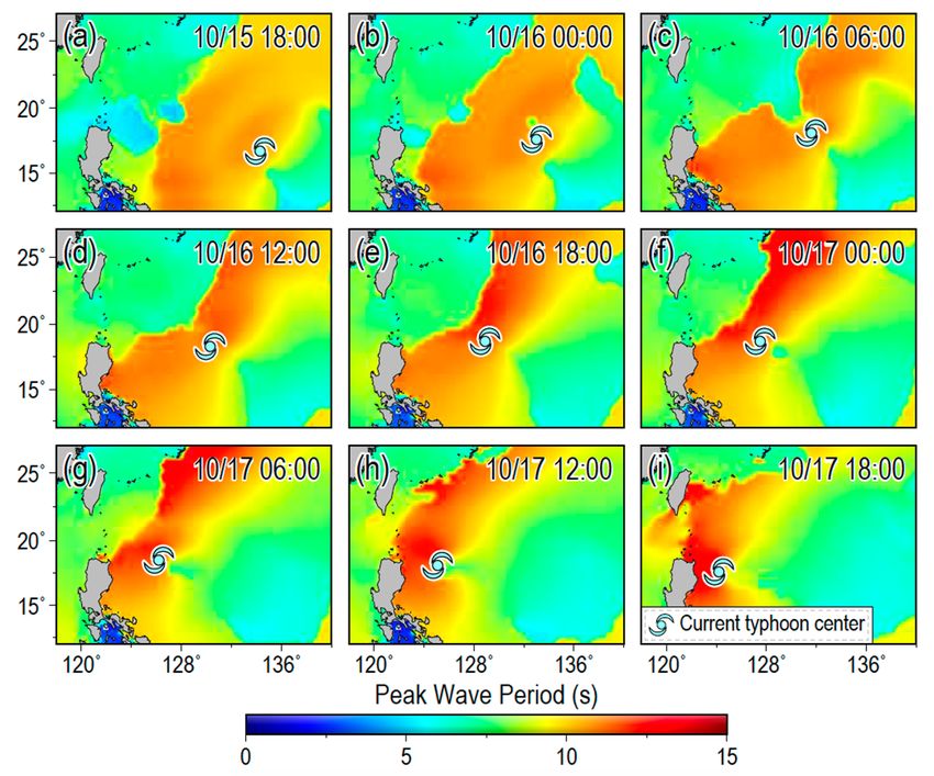
Remote Sens. 2018, 10, x FOR PEER REVIEW 7 of 15
window for2018,
Remote Sens. the 10,
FrFT
1437calculation was set to three hours, during which we assumed that the swell
7 of 15
origin was quasi-constant in time and space.
Figure
Figure3.3.Schematic
Schematicofof(a)(a)DF
DFmicroseism
microseismgeneration
generationbybytyphoon-induced
typhoon-inducedswells,
swells,and
and(b)
(b)dispersive
dispersive
DFDFmicroseisms theywould
microseisms as they would appear
appear on aon a spectrogram.
spectrogram. WhenWhen the typhoon-induced
the typhoon-induced swells
swells propagate
through through
propagate deep water
deepoverwaterlong
overdistances, high-frequency
long distances, components
high-frequency traveltravel
components moremoreslowly than
slowly
low-frequency
than components,
low-frequency and consequently,
components, the observedthe
and consequently, DF microseisms
observed DF are frequency-dispersed,
microseisms are
with an energy distribution
frequency-dispersed, with an (pink
energyellipse) tilting from
distribution (pinklower-left to upper-right.
ellipse) tilting For interpretation,
from lower-left to upper-right.see
theinterpretation,
For text. see the text.
3.2.Fractional
3.2. FractionalFourier
FourierTransform
Transform
Thefractional
The fractional Fourier
Fourier transform
transform(FrFT)
(FrFT)was
wasintroduced
introducedby by
Namias [40] [40]
Namias and is now
and is widely applied
now widely
in various fields of study as a rotation operator in the time–frequency plane [41,42]. The
applied in various fields of study as a rotation operator in the time–frequency plane [41,42]. The FrFT is suitable
for analyzing
FrFT is suitablelinear
for frequency-modulated (LFM) signals due(LFM)
analyzing linear frequency-modulated to theirsignals
energy dueconcentration, as they
to their energy
concentration, as they have linear instantaneous frequencies in a subregion of their total bandwidth.by
have linear instantaneous frequencies in a subregion of their total bandwidth. The FrFT is defined
the transformation kernel Kα (t, u); for an LFM signal x (t), this can be expressed by
The FrFT is defined by the transformation kernel K α (t ,u); for an LFM signal x(t ) , this can be
Z ∞
expressed by Xα ( u ) = x (t)Kα (t, u)dt, (7)
−∞
∞
X (u) =
x(t)K
t2 +u2 (t ,u)dttu,
√ (7)
α −∞ ( 2 αcot α − sin α ))
1 − i cot α exp(i2π α 6= nπ
Kα (t, u) = δ(t − u) α = 2nπ , (8)
t 2 + u2 tu
1− icot α exp(i2π ( cot α − )) α = (2nα+ ≠1)nππ
δ(t + u)
2 sin α
where α is the angle used to apply a rotational transformation to the conventional time–frequency
axes. The optimal
δ (t − u)
K α (t ,u) =αvalue yields the highest-magnitude α = 2nπ ,
response to the LFM signal. According(8) to
δ (tα +is u)
Reference [43], the optimal transform angle α =of(2n+1)
numerically related to the rate π signal χ by
the LFM
Fs2 /Ω
α = −arctan( ), (9)
2χ
where α is the angle used to apply a rotational transformation to the conventional time–frequency
axes.
whereTheF optimal α value yields the highest-magnitude response to the LFM signal. According to
s is the sampling rate and Ω is the total number of time samples. The frequency-versus-time
Reference [43],paper,
slope in this the optimal
d f /dt, transform
was computed α χis according
anglefrom numerically related to(9).
to Equation the rate of the LFM signal
χ by
4. Results and Discussion
Fs2 /Ω
4.1. Swell-Generated DF Microseisms α = −arctan( ), (9)
2χ
The DF microseisms generated by Typhoon Megi were detected effectively on spectrograms
(Figure F2),
where s
is the
with little sampling
contamination. and Ω high-amplitude
rate Occasional is the total transient
number events,
of timesuchsamples. The
as earthquakes,
instrumental irregularities,
frequency-versus-time and
slope in non-stationary
this paper, df /dtnoise, appeared
, was as from
computed χ according
short pulses on the spectrograms.
to Equation
Before 17 October 2010, when the typhoon center was still over the deep Philippine Sea (Figure 1), we
(9).
4.1. Swell-Generated DF Microseisms
The DF microseisms generated by Typhoon Megi were detected effectively on spectrograms
(Figure 2), with little contamination. Occasional high-amplitude transient events, such as
Remote Sens. 2018, 10, 1437 8 of 15
earthquakes, instrumental irregularities, and non-stationary noise, appeared as short pulses on the
spectrograms. Before 17 October 2010, when the typhoon center was still over the deep Philippine
Seaobserved weak
(Figure 1), weDF microseisms
observed weak above 0.2 Hz, which
DF microseisms abovewere
0.2shown to have
Hz, which wereClass-I
shown source mechanisms
to have Class-I
and centroids
source mechanisms around
and the typhoon
centroids centerthe
around [28].
typhoon center [28].
Figure
Figure 4 shows
4 shows thethe distributions
distributions of of
thethe peak
peak periods
periods of of ocean
ocean waves
waves when
when Typhoon
Typhoon Megi
Megi was
was
still
still over
over thethe Philippine
Philippine Sea.
Sea. The
The majority
majority of of typhoon-induced
typhoon-induced swells
swells propagated
propagated nearly
nearly westward,
westward,
to to
Taiwan
Taiwan and
and Luzon
Luzon islands. Because
islands. Becauseof of
thethedispersive
dispersive effects of of
effects surface
surfacegravity waves
gravity waves onondeep
deep
water,
water,thethe
low-frequency
low-frequency waves
waves(deep redred
(deep color in in
color Figure
Figure 4) 4)
propagated
propagated at at
a higher
a highergroup
groupvelocity
velocity
than
thanthethe
high-frequency
high-frequency components,
components,thus arrived
thus arrivedand interacted
and interacted earlier with
earlier withthethe
coasts to to
coasts generate
generate
low-frequency
low-frequency DFDFmicroseisms.
microseisms.
Figure
Figure 4. Analysis
4. Analysis of propagation
of the the propagation and dispersion
and dispersion of ocean
of ocean swellsswells induced
induced by Typhoon
by Typhoon Megi.
Megi. The
The distribution
distribution of peakofperiods
peak periods
of oceanofwaves
ocean in
waves in 6-h
6-h time time intervals
intervals onOctober
on 15–17 15–17 October 2010
2010 (a–i) (a–i)
was
was predicted
predicted by ERA5by ERA5 reanalysis
reanalysis from from the European
the European Centre
Centre for for Medium-Range
Medium-Range Weather
Weather Forecasts
Forecasts
(ECMWF),
(ECMWF), and
and hurricane
hurricane symbols
symbols indicate
indicate thethe location
location of of
thethe typhoon
typhoon center
center at at each
each time.
time.
DFDFmicroseisms
microseismswere
were observed
observed on on17–18
17–18October 20102010
October with with
dominant frequencies
dominant that increased
frequencies that
increased almost linearly from 0.12 to 0.20 Hz (Figure 2). In our preliminary study [28],that
almost linearly from 0.12 to 0.20 Hz (Figure 2). In our preliminary study [28], we noted we these
notedDF
microseisms
that were expected
these DF microseisms wereto originate
expected near local coasts
to originate near (i.e.,
localalong
coaststhe SE along
(i.e., coast oftheTaiwan) due
SE coast of to
interactions
Taiwan) due tobetween reflected
interactions ocean
between swells and
reflected oceansubsequent
swells andincident swells.
subsequent This isswells.
incident consistent
Thiswith
is
consistent with the propagation of typhoon-induced swells shown in Figure 4. The onset of theseDF
the propagation of typhoon-induced swells shown in Figure 4. The onset of these dispersive
microseisms
dispersive in the late afternoon
DF microseisms ofafternoon
in the late 17 Octoberof2010 was in good
17 October 2010 wasagreement
in goodwith the timewith
agreement when thethe
firstwhen
time low-frequency swells arrived atswells
the first low-frequency the eastern coastline
arrived at theofeastern
Taiwan.coastline
The time–frequency
of Taiwan.characteristics
The time–
of these DF microseisms reflect the dispersion of the corresponding ocean
frequency characteristics of these DF microseisms reflect the dispersion of the corresponding swells, and could, ocean
thus, be
used as
swells, a proxy
and could,to thus,
explore bethe generation
used and propagation
as a proxy to exploreofthe typhoon-induced
generation and swells.
propagation of
typhoon-induced swells.
4.2. Origins of Typhoon-Induced Swell
The of
4.2. Origins derived propagation
Typhoon-Induced distances of the typhoon-induced swells were compared with the
Swell
distances from the seismic stations to the typhoon centers indicated by the best-track data (Figure 5).
The correlation coefficients (CC) between the least-squares regression lines (pink lines in Figure 5a–f)
and the corresponding dominant energy points (i.e., the points (t, f ) with the highest spectral
amplitude S(t, f ) at each time t) in the inspected region were all above 0.8, indicating linear dispersion
of the DF microseisms. However, when the slope of the least-squares regression line was used in
Equation (5) directly, we found that the estimated swell source regions were located at a distance
(~1000 km) from the trajectory of Megi (Figure 5g–l). It is likely that the typhoon moved significantly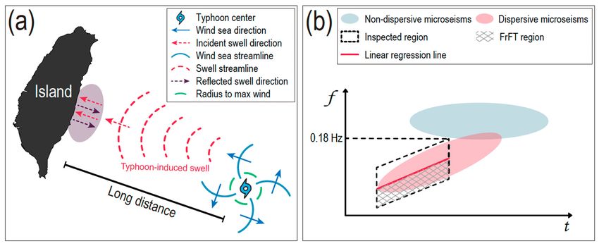
distances from the seismic stations to the typhoon centers indicated by the best-track data (Figure 5).
The correlation coefficients (CC) between the least-squares regression lines (pink lines in Figure 5a–
f) and the corresponding dominant energy points (i.e., the points (t , f ) with the highest spectral
amplitude S(t , f ) at each time t ) in the inspected region were all above 0.8, indicating linear
dispersion of the
Remote Sens. 2018,DF
10, microseisms.
1437 However, when the slope of the least-squares regression line was 9 of 15
used in Equation (5) directly, we found that the estimated swell source regions were located at a
distance (~1000 km) from the trajectory of Megi (Figure 5g–l). It is likely that the typhoon moved
over this over
significantly longthis
timelong
interval, and the and
time interval, induced ocean waves,
the induced thus, developed
ocean waves, into ocean
thus, developed swells at
into ocean
swells at locations far from the typhoon trajectory. Therefore, the inspected region was segmentedinto
locations far from the typhoon trajectory. Therefore, the inspected region was segmented
intothree-hour
three-hour timetime windows, during
during which
whichthethetyphoon
typhoonwaswasassumed
assumed to to
movemove minimally
minimally andand
the the
swell origin was constrained to a quasi-static region in space and time. The FrFT
swell origin was constrained to a quasi-static region in space and time. The FrFT was then computedwas then computed
for for
eacheach successive
successive segmentofof DF
segment DF microseisms
microseismstotoobtain
obtainthethe
corresponding
corresponding swell propagation
swell distance.
propagation
We find
distance. Wethatfindthese
thatdistances are generally
these distances coincident
are generally with thewith
coincident locations of the typhoon
the locations center after
of the typhoon
15 October 2010, when Megi strengthened to become a typhoon (Figure
center after 15 October 2010, when Megi strengthened to become a typhoon (Figure 5g–l). 5g–l).
Figure 5. Estimation
Figure of the
5. Estimation propagation
of the propagation distance x xofoftyphoon-induced
distance typhoon-inducedswellsswellsfrom
fromthe
theorigin
origin to
to the
the Taiwan coastline
coastline based
based ononseismic
seismicrecords.
records.(a–f)
(a–f)Dispersive
DispersiveDF DFmicroseisms
microseismsgenerated
generated byby
thethe
ocean
ocean swells
swells induced
induced byby Typhoon
Typhoon Megi Megi on power
on power spectrograms
spectrograms computed
computed usingusing
datadata
fromfrom seismic
seismic stations
stations in Taiwan. The pink solid lines superimposed on the spectrograms represent least-squares
in Taiwan. The pink solid lines superimposed on the spectrograms represent least-squares regression
regression
lines as lines as in
in Figure 3b, Figure
and dark3b,lines
anddenote
dark the
lines denote slope
calculated the calculated
d f /dt of theslope df /dt
dispersive of the
DF microseisms
in successive
dispersive three-hour time
DF microseisms windows. (g–l)
in successive Comparison
three-hour time between
windows.estimated propagationbetween
(g–l) Comparison distances of
typhoon-induced swells and distances from the typhoon center to seismic stations
estimated propagation distances of typhoon-induced swells and distances from the typhoon center(red lines). Large
to seismic stations (red lines). Large pink dots and small gray dots represent calculated propagationlines
pink dots and small gray dots represent calculated propagation distances using the pink and dark
in theusing
distances subfigures in the
the pink andleft column,
dark respectively.
lines in the subfigures in the left column, respectively.
Figure 6 shows the propagation distance x, the initial wave period T, and the origin time t2 of the
typhoon-induced swells derived from the dispersion characteristics of DF microseisms recorded by
station YULB, which is located close to the coastline (~18 km) of eastern Taiwan (Figure 1). Probable
source regions are indicated by dotted circles with their centers at the station location and their radii
equal to the propagation distance x. We assumed that the most likely source regions of long-period
ocean swells had the highest-amplitude significant wave heights, and therefore, we superimposed2
of the typhoon-induced swells derived from the dispersion characteristics of DF microseisms
recorded by station YULB, which is located close to the coastline (~18 km) of eastern Taiwan (Figure
1). Probable source regions are indicated by dotted circles with their centers at the station location
and their radii equal to the propagation distance x . We assumed that the most likely source regions
Remote Sens. 2018, 10, 1437 10 of 15
of long-period ocean swells had the highest-amplitude significant wave heights, and therefore, we
superimposed the significant height of the total swell predicted by ERA5 reanalysis at time t 1 ,
the significant height of the total swell predicted by ERA5 reanalysis at time t1 , which was close to
which was close swell
the calculated to the calculated
origin swell
time t2 , in Figureorigin
6a–c. time t 2 , in the
Furthermore, Figure 6a–c. Furthermore,
corresponding peak wave the
period,
which reports
corresponding thewave
peak waveperiod,
fronts which
of the long-period oceanfronts
reports the wave swells,ofwas
the superimposed on the
long-period ocean plots of
swells,
wasFigure 6d–f. Weon
superimposed compared
the plots the origins6d–f.
of Figure of typhoon-induced
We compared theswells calculated
origins from DF microseisms
of typhoon-induced swells
with ocean-wave
calculated state data provided
from DF microseisms by ERA5state
with ocean-wave reanalysis and found
data provided good reanalysis
by ERA5 consistency between
and found the
goodtwoconsistency between
estimates. These resultsthe two that
indicate estimates. These characteristics
the dispersion results indicateof DFthat the dispersion
microseisms recorded by
characteristics of DF
coastal seismic microseisms
stations could be recorded
a useful by coastal
proxy seismic stations
for tracking could betyphoon-induced
and monitoring a useful proxy for
swells
tracking
over and monitoring typhoon-induced swells over oceans.
oceans.
Figure
Figure 6. Typhoon-induced
6. Typhoon-induced swellswell propagation
propagation calculated
calculated fromfrom dispersive
dispersive DF microseisms
DF microseisms at station
at station
YULB,
YULB, compared
compared withwith(a–c)(a–c) significant
significant heights
heights of total
of total swells
swells andand (d–f)
(d–f) peak
peak wave
wave periods
periods at at time t1
time
t 1 as predicted by ERA5 reanalysis. The dotted circle centered on station YULB, with radius equal
as predicted by ERA5 reanalysis. The dotted circle centered on station YULB, with radius equal to
the propagation distance x, represents the probable location of the origin of each swell. The origin
to the propagation
time distance
and initial wave periodx , of
represents the probableswell
the typhoon-induced location of the origin
are denoted t2 and of
T, each swell. The
respectively, and the
hurricane
origin time andsymbols
initialindicate
wave the locations
period of the
of the typhoon center. swell are denoted t and
typhoon-induced
2
T ,
respectively,
4.3. andDeviations
Localization the hurricane symbols indicate the locations of the typhoon center.
The effective generation of dispersive DF microseisms depends on the properties of the coastlines,
where reflected and incident typhoon-induced swells interact to generate DF microseisms. For example,
the DF microseisms that we observed were weaker in the Ryukyu Islands than in Taiwan, as shown in
Figure 2. It is likely that the coastlines of the Ryukyu Islands are not long enough to produce the strong
reflections necessary for strong DF microseisms. Consequently, coastal seismic stations in eastern
Taiwan, such as station YULB, were primarily used in this study. In addition, the geometry of theThe effective generation of dispersive DF microseisms depends on the properties of the
coastlines, where reflected and incident typhoon-induced swells interact to generate DF
microseisms. For example, the DF microseisms that we observed were weaker in the Ryukyu Islands
than in Taiwan, as shown in Figure 2. It is likely that the coastlines of the Ryukyu Islands are not
long enough to produce the strong reflections necessary for strong DF microseisms. Consequently,11 of 15
Remote Sens. 2018, 10, 1437
coastal seismic stations in eastern Taiwan, such as station YULB, were primarily used in this study.
In addition, the geometry of the coastlines has a strong influence on the generation of DF
coastlines
microseisms has
[44], asasuch
strong influence oncan
microseisms theonly
generation of DF microseisms
be generated [44], as
effectively when such microseisms
incident can only
ocean swells
are reflected in the opposite direction by the coast, and subsequently, interfere with later incident coast,
be generated effectively when incident ocean swells are reflected in the opposite direction by the
swells.and subsequently,
Figure 7 showsinterfere
several with later incident
coastline geometriesswells.
thatFigure
could 7 contribute
shows several coastlinetogeometries
effectively the
that could
generation of DFcontribute
microseisms. effectively to the generation
The topographic propertiesof of
DFthe microseisms. The as
coastlines, such topographic
steepness, properties
will
of thethe
also affect coastlines,
reflectionsuch as steepness,
coefficients will also swells
of incident affect the
andreflection
further coefficients of incidentofswells
affect the efficiency the and
further
generation ofaffect the efficiency as
DF microseisms, of the generation
described by of DF microseisms,
Ardhuin as In
et al. [33]. described
addition,by the
Ardhuin et al. [33].
effective
In addition,
generation the effective
of dispersive generationdepends
DF microseisms of dispersive
on the DF microseisms
intensity dependsocean
of the incident on the intensity
swells; e.g., of the
beforeincident ocean swells;into
Megi strengthened e.g.,abefore
typhoon,Megiitsstrengthened
induced ocean intowaves
a typhoon, its induced
and swells were ocean waves and
not strong
enoughswells were not
to generate DFstrong enoughattohigh
microseisms generate DF microseisms
signal-to-noise at high in
ratios (SNRs) signal-to-noise ratios (SNRs) in
Taiwan. Consequently,
Taiwan. swell
the computed Consequently,
propagationthe distances
computedwere swell propagation
not so consistent distances
with thewere not soofconsistent
locations the typhoonwith the
centerlocations of thebefore
for the period typhoon center for2010
15 October the (Figure
period before
5). 15 October 2010 (Figure 5).
FigureFigure 7. Examples
7. Examples of coastlinegeometries
of coastline geometries that
that facilitate
facilitatethe generation
the of dispersive
generation DF microseisms,
of dispersive DF
microseisms, including (a) straight coast, (b) rectangular coast, (c) bay, and (d) channel. In cases,
including (a) straight coast, (b) rectangular coast, (c) bay, and (d) channel. In all the coast
all cases,
the coast provides opportunities for interference between incident and reflected ocean waves withsimilar
provides opportunities for interference between incident and reflected ocean waves with
similarperiods.
periods.Landscape
Landscapeimages
imageswere
weredownloaded
downloadedfromfromGoogle
GoogleMaps.
Maps.
Furthermore, the geographic locations of seismic stations have considerable influence on the
Furthermore, the geographic locations of seismic stations have considerable influence on the
effectiveness of our method for tracking typhoon-induced swells. Figure 8 shows a possible source of
effectiveness of our method for tracking typhoon-induced swells. Figure 8 shows a possible source
error in our localization method caused by the location of a seismic station relative to the coast. The
of error in our localization method caused by the location of a seismic station relative to the coast.
calculated propagation distance x of the typhoon-induced swell is theoretically expected to equal the
true propagation distance r from the swell source region to the coastal source of the DF microseisms.
However, in the localization process, the derived source regions of ocean swells are restricted to an
arc of radius x centered on the seismic station rather than the coast. Hence, the distance vector from
the seismic station to the source of the DF microseisms contributes to the localization misfit. Further
investigation of the coastal source regions of the dispersive DF microseisms is necessary to evaluate
and correct these deviations, and such an effort is essential to improve this method.microseisms. However, in the localization process, the derived source regions of ocean swells are
restricted to an arc of radius x centered on the seismic station rather than the coast. Hence, the
distance vector from the seismic station to the source of the DF microseisms contributes to the
localization misfit. Further investigation of the coastal source regions of the dispersive DF
microseisms
Remote is10,
Sens. 2018, necessary
1437 to evaluate and correct these deviations, and such an effort is essential to
12 of 15
improve this method.
Figure
Figure 8. Schematic diagram
8. Schematic diagram of of the
the analysis
analysis of
of the
the ocean
ocean swell
swell localization
localization deviation
deviation due
due to
to the
the
geographic location of the seismic station.
geographic location of the seismic station.
From our preliminary investigation [28], DF microseisms with coastal sources propagate inland
From our preliminary investigation [28], DF microseisms with coastal sources propagate inland
and gradually attenuate; thus, coastal stations generally record stronger DF microseisms than inland
and gradually attenuate; thus, coastal stations generally record stronger DF microseisms than inland
sites. Therefore, the distance inland of the seismic station plays an important role in determining
sites. Therefore, the distance inland of the seismic station plays an important role in determining the
the SNR. For example, stations located relatively close to the eastern coast of Taiwan, such as YULB,
SNR. For example, stations located relatively close to the eastern coast of Taiwan, such as YULB,
NACB, and TWGB, detected stronger dispersive DF microseisms (Figures 2 and 5). This is one of the
NACB, and TWGB, detected stronger dispersive DF microseisms (Figures 2 and 5). This is one of the
principal reasons why station YULB was used in this study. In addition, the detection and calculation
principal reasons why station YULB was used in this study. In addition, the detection and
of dispersive DF microseisms are affected by local background noise, including undesirable signals
calculation of dispersive DF microseisms are affected by local background noise, including
induced by local site effects.
undesirable signals induced by local site effects.
Finally, localization deviations could also be affected by the accuracy of the fundamental
Finally, localization deviations could also be affected by the accuracy of the fundamental
assumptions of this method. The ocean swell propagation distance x is calculated from the frequency
assumptions of this method. The ocean swell propagation distance x is calculated from the
dispersion relationship of the ocean swells, and is directly used in computing the great-circle distance
frequency dispersion relationship of the ocean swells, and is directly used in computing the
from the observation site to the swell source region. However, the actual propagation route of the
great-circle distance from the observation site to the swell source region. However, the actual
swells can be affected by factors including sea surface winds, ocean currents, wave–wave interactions,
propagation route of the swells can be affected by factors including sea surface winds, ocean
and seafloor topography near the coast, leading to deviations of the propagation path from an idealized
currents, wave–wave interactions, and seafloor topography near the coast, leading to deviations of
great circle. As a result, as typhoon-induced swells propagate farther, and these factors increasingly
the propagation path from an idealized great circle. As a result, as typhoon-induced swells
affect the deviation, resulting in larger errors in the localization of swell source regions, as shown
propagate farther, and these factors increasingly affect the deviation, resulting in larger errors in the
in Figure 5.
localization of swell source regions, as shown in Figure 5.
5. Conclusions
5. Conclusions
Ocean swells induced in the western Pacific Ocean by Typhoon Megi in 2010 were tracked
effectively using DF microseisms recorded by seismic stations in eastern Taiwan. The frequency
dispersion of the DF microseisms was used to calculate the propagation distance and constrain the
source regions of ocean swells. Localized source regions and calculated wave periods of ocean swells
were generally consistent with ocean-wave field data provided by ERA5 reanalysis from ECMWF.
Although localization results can depend on the effective detection of dispersive DF microseisms,
which is tied to both coastline geometry and the locations of the seismometers, the present resultsRemote Sens. 2018, 10, 1437 13 of 15
indicate that the dispersion characteristics of DF microseisms recorded by coastal seismometers could
be a viable proxy measure for tracking and monitoring typhoon-induced swells across the oceans.
Author Contributions: Conceptualization, J.L., X.L., and H.Z. Data curation, S.F. Formal analysis, J.L., S.F.,
and H.Z. Investigation, S.F. Methodology, J.L. and H.Z. Project administration, J.L. Supervision, J.L. and X.L.
Visualization, S.F. and R.W. Writing—original draft, J.L. Writing—review and editing, J.L., X.L., and H.Z.
Acknowledgments: Seismic waveform data used in this study are freely available from the IRIS Data Management
System (www.iris.edu) and the F-net network of Japan (www.fnet.bosai.go.jp). MODIS data are provided by
NASA (National Aeronautics and Space Administration, USA). ERA5 reanalysis of ocean wave data from ECMWF
was accessed at http://apps.ecmwf.int/data-catalogues/era5. The best-track data of the RSMC were accessed at
http://www.jma.go.jp/jma/jma-eng/jma-center/rsmc-hp-pub-eg/RSMC_HP.htm. Some of the figures were
generated using the Generic Mapping Tools (GMT) software [45]. The manuscript benefited from thoughtful
discussions with Hanhao Zhu. This work was supported by the Natural Science Foundation of Zhejiang Province
(LZ14D060001). The views, opinions, and findings contained in this report are those of the authors and should not
be construed as an official NOAA or US Government position, policy, or decision.
Conflicts of Interest: The authors declare no conflicts of interest.
References
1. Snodgrass, F.E.; Groves, G.W.; Hasselmann, K.; Miller, G.R.; Munk, W.H.; Powers, W.H. Propagation of ocean
swell across the Pacific. Philos. Trans. R. Soc. Lond. Ser. A 1966, 249, 431–497. [CrossRef]
2. Ardhuin, F.; Chapron, B.; Collard, F. Observation of swell dissipation across oceans. Geophys. Res. Lett.
2009, 36. [CrossRef]
3. Grachev, A.A.; Fairall, C.W. Upward momentum transfer in the marine boundary layer. J. Phys. Oceanogr.
2001, 31, 1698–1711. [CrossRef]
4. Babanin, A.V. On a wave-induced turbulence and a wave-mixed upper ocean layer. Geophys. Res. Lett. 2006,
33. [CrossRef]
5. Hwang, P.A. Observations of swell influence on ocean surface roughness. J. Geophys. Res. 2008, 113.
[CrossRef]
6. Semedo, A. Atmosphere-Ocean Interactions in Swell Dominated Wave Fields. Available online: http://www.
diva-portal.org/smash/record.jsf?pid=diva2%3A350126&dswid=4604 (accessed on 6 September 2018).
7. Wu, L.; Rutgersson, A.; Sahlee, E.; Guo Larsen, X. Swell impact on wind stress and atmospheric mixing in a
regional coupled atmosphere-wave model. J. Geophys. Res. Oceans 2016, 121, 4633–4648. [CrossRef]
8. Smedman, A.S.; Högström, U.; Sahleé, E.; Drennan, W.M.; Kahma, K.K.; Pettersson, H.; Zhang, F.
Observational study of marine atmospheric boundary layer characteristics during swell. J. Atmos. Sci.
2009, 66, 2747–2763. [CrossRef]
9. Högström, U.; Smedman, A.S.; Semedo, A.; Rutgersson, A. Comments on “A global climatology of
wind-wave interaction”. J. Phys. Oceanogr. 2011, 41, 1811–1813. [CrossRef]
10. Li, X.; Zhang, J.A.; Yang, X.; Pichel, W.G.; DeMaria, M.; Long, D.; Li, Z. Tropical cyclone morphology from
spaceborne synthetic aperture radar. Bull. Am. Meteorol. Soc. 2012, 94, 215–230. [CrossRef]
11. Li, X. The first Sentinel-1 SAR image of a typhoon. Acta Oceanol. Sin. 2015, 34. [CrossRef]
12. Li, X.; Pichel, W.G.; He, M.; Wu, S.; Friedman, K.S.; Clemente-Colon, P.; Zhao, C. Observation of
hurricane-generated ocean swell refraction at the Gulf Stream north wall with the RADARSAT-1 synthetic
aperture radar. IEEE Trans. Geosci. Remote Sens. 2002, 40, 2131–2142.
13. Jiang, H.; Stopa, J.E.; Wang, H.; Husson, R.; Mouche, A.; Chapron, B.; Chen, G. Tracking the attenuation and
nonbreaking dissipation of swells using altimeters. J. Geophys. Res. Oceans 2016, 121, 1446–1458. [CrossRef]
14. Hasselmann, K.; Barnett, T.P.; Bouws, E.; Carlson, H.; Gartwright, D.E.; Enke, K.; Ewing, J.A.; Gienapp, H.;
Hasselmann, D.E.; Kruseman, P.; et al. Meansurements of wind-wave growth and swell decay during the
Joint North Sea Wave Project (JONSWAP). Dtsch. Hydrogr. Z. Suppl. 1973, 12, 1–95.
15. Bromirski, P.D.; Flick, R.E.; Graham, N. Ocean wave height determined from inland seismometer data:
Implications for investigating wave climate changes in the NE Pacific. J. Geophys. Res. Oceans 1999, 104,
20753–20766. [CrossRef]
16. Okal, E.A.; MacAyeal, D.R. Seismic recording on drifting icebergs: Catching seismic waves, tsunamis and
storms from Sumatra and elsewhere. Seismol. Res. Lett. 2006, 77, 659–671. [CrossRef]Remote Sens. 2018, 10, 1437 14 of 15
17. Barruol, G.; Reymond, D.; Fontaine, F.R.; Hyvernaud, O.; Maurer, V.; Maamaatuaiahutapu, K. Characterizing
swells in the southern Pacific from seismic and infrasonic noise analyses. Geophys. J. Int. 2006, 164, 516–542.
[CrossRef]
18. Barruol, G.; Davy, C.; Fontaine, F.R.; Schlindwein, V.; Sigloch, K. Monitoring austral and cyclonic swells in
the “Iles Eparses” (Mozambique channel) from microseismic noise. Acta Oecol. 2016, 72, 120–128. [CrossRef]
19. Cathles IV, L.M.; Okal, E.A.; MacAyeal, D.R. Seismic observations of sea swell on the floating Ross Ice Shelf,
Antarctica. J. Geophys. Res. Earth Surf. 2009, 114. [CrossRef]
20. Davy, C.; Barruol, G.; Fontaine, F.R.; Cordier, E. Analyses of extreme swell events on La Réunion Island from
microseismic noise. Geophys. J. Int. 2016, 207, 1767–1782. [CrossRef]
21. Haubrich, R.A.; McCamy, K. Microseisms: Coastal and pelagic sources. Rev. Geophys. 1969, 7, 539–571.
[CrossRef]
22. Bromirski, P.D. Vibrations from the “Perfect Storm”. Geochem. Geophy. Geosyst. 2001, 2. [CrossRef]
23. Bromirski, P.D.; Duennebier, F.K.; Stephen, R.A. Mid-ocean microseisms. Geochem. Geophy. Geosyst. 2005, 6.
[CrossRef]
24. Longuet-Higgins, M.S. A theory of the origin of microseisms. Philos. Trans. R. Soc. Lond. Ser. A Math.
Phys. Sci. 1950, 243, 1–35. [CrossRef]
25. Gerstoft, P.; Fehler, M.C.; Sabra, K.G. When Katrina hit California. Geophys. Res. Lett. 2006, 33. [CrossRef]
26. Gerstoft, P.; Shearer, P.M.; Harmon, N.; Zhang, J. Global P, PP, and PKP wave microseisms observed from
distant storms. Geophys. Res. Lett. 2008, 35. [CrossRef]
27. Zhang, J.; Gerstoft, P.; Bromirski, P.D. Pelagic and coastal sources of P-wave microseisms: Generation under
tropical cyclones. Geophys. Res. Lett. 2010, 37. [CrossRef]
28. Lin, J.M.; Lin, J.; Xu, M. Microseisms generated by super typhoon Megi in the western Pacific Ocean.
J. Geophys. Res. Oceans 2017, 122, 9518–9529. [CrossRef]
29. Tanimoto, T.; Lin, C.J.; Hadziioannou, C.; Igel, H.; Vernon, F. Estimate of Rayleigh-to-Love wave ratio in the
secondary microseism by a small array at Piñon Flat observatory, California. Geophys. Res. Lett. 2016, 43.
[CrossRef]
30. Nishida, K.; Takagi, R. Teleseismic S wave microseisms. Science 2016, 353, 919–921. [CrossRef] [PubMed]
31. Hasselmann, K.A. Statistical analysis of the generation of microseisms. Rev. Geophys. 1963, 1, 177–210.
[CrossRef]
32. Webb, S.C. Broadband seismology and noise under the ocean. Rev. Geophys. 1998, 36, 105–142. [CrossRef]
33. Ardhuin, F.; Stutzmann, E.; Schimmel, M.; Mangeney, A. Ocean wave sources of seismic noise. J. Geophys.
Res. 2011, 116. [CrossRef]
34. Chi, W.C.; Chen, W.J.; Kuo, B.Y.; Dolenc, D. Seismic monitoring of western Pacific typhoons. Mar. Geophys.
Res. 2010, 31, 239–251. [CrossRef]
35. Sufri, O.; Koper, K.D.; Burlacu, R.; Foy, B.D. Microseisms from Superstorm Sandy. Earth Planet. Sci. Lett.
2014, 402, 324–336. [CrossRef]
36. Lin, J.M.; Wang, Y.T.; Wang, W.T.; Li, X.F.; Fang, S.K.; Chen, C.; Zheng, H. Seismic Remote Sensing of
Super Typhoon Lupit (2009) with Seismological Array Observation in NE China. Remote Sens. 2018, 10, 235.
[CrossRef]
37. Gray, W.M. Global view of the origin of tropical disturbances and storms. Mon. Weather Rev. 1968, 96,
669–700. [CrossRef]
38. Lu, X.; Yu, H.; Yang, X.; Li, X. Estimating tropical cyclone size in the Northwestern Pacific from geostationary
satellite infrared images. Remote Sens. 2017, 9, 728. [CrossRef]
39. Munk, W.H.; Miller, G.R.; Snodgrass, F.E.; Barber, N.F. Directional recording of swell from distant storms.
Philos. Trans. R. Soc. Lond. Ser. A 1963, 255, 505–584. [CrossRef]
40. Namias, V. The fractional order Fourier transform and its application to quantum mechanics. IMA J.
Appl. Math. 1980, 25, 241–265. [CrossRef]
41. Yu, J.; Zhang, L.; Liu, K.; Liu, D. Separation and localization of multiple distributed wideband chirps using
the fractional Fourier transform. EURASIP J. Wirel. Commun. Netw. 2015, 1, 1–8. [CrossRef]
42. Wei, D.; Li, Y.M. Generalized sampling expansions with multiple sampling rates for lowpass and bandpass
signals in the fractional Fourier transform domain. IEEE Trans. Signal Process. 2016, 64, 4861–4874. [CrossRef]
43. Capus, C.; Brown, K. Short-time fractional Fourier methods for the time-frequency representation of chirp
signals. J. Acoust. Soc. Am. 2003, 113, 3253–3263. [CrossRef] [PubMed]You can also read