Long-Term Monitoring of Cropland Change near Dongting Lake, China, Using the LandTrendr Algorithm with Landsat Imagery
←
→
Page content transcription
If your browser does not render page correctly, please read the page content below
remote sensing
Article
Long-Term Monitoring of Cropland Change near
Dongting Lake, China, Using the LandTrendr
Algorithm with Landsat Imagery
Lihong Zhu, Xiangnan Liu *, Ling Wu, Yibo Tang and Yuanyuan Meng
 School of Information Engineering, China University of Geosciences, Beijing 100083, China;
 zhulh@cugb.edu.cn (L.Z.); wuling@cugb.edu.cn (L.W.); delicktang@cugb.edu.cn (Y.T.);
 mengyy@cugb.edu.cn (Y.M.)
 * Correspondence: liuxn@cugb.edu.cn; Tel.: +86-10-8232-3056

 Received: 13 April 2019; Accepted: 22 May 2019; Published: 24 May 2019

 Abstract: Tracking cropland change and its spatiotemporal characteristics can provide a scientific
 basis for assessments of ecological restoration in reclamation areas. In 1998, an ecological restoration
 project (Converting Farmland to Lake) was launched in Dongting Lake, China, in which original lake
 areas reclaimed for cropland were converted back to lake or to poplar cultivation areas. This study
 characterized the resulting long-term (1998–2018) change patterns using the LandTrendr algorithm
 with Landsat time-series data derived from the Google Earth Engine (GEE). Of the total cropland
 affected, ~447.48 km2 was converted to lake and 499.9 km2 was converted to poplar cultivation,
 with overall accuracies of 87.0% and 83.8%, respectively. The former covered a wider range,
 mainly distributed in the area surrounding Datong Lake, while the latter was more clustered in
 North and West Dongting Lake. Our methods based on GEE captured cropland change information
 efficiently, providing data (raster maps, yearly data, and change attributes) that can assist researchers
 and managers in gaining a better understanding of environmental influences related to the ongoing
 conversion efforts in this region.

 Keywords: cropland change patterns; LandTrendr algorithm; Landsat time series; Google Earth
 Engine; Dongting Lake; China

1. Introduction
     Dongting Lake, once the largest freshwater lake in China, has shrunk to the second-largest due
to land reclamation for agriculture; this has resulted in serious ecological degradation of the area’s
wetlands [1]. After the devastating flood in 1998, the government promoted the project of Converting
Farmland to Lake (CFTL) and planned to abandon 785.7 km2 of cropland area, where conversion
to lake or poplar trees cultivation could establish a new balance between economic benefits and the
regulation of wetland ecological functions. These efforts have created a need for long-term monitoring
of cropland change processes to provide scientific data for ongoing ecological management after
project completion.
     Although field surveys are the most accurate monitoring method for this purpose, they are
impractical over large areas due to time constraints and the inability to assess certain inaccessible sites
(such as shoal areas). In contrast, remote sensing techniques enable frequent imaging, easier access,
and larger-scale monitoring, becoming important global data sources for detecting environmental
changes (including those to cropland) [2–4]. The moderate resolution of publicly available USGS
Landsat data [5] makes them suitable for monitoring changes in agriculture fields [6–8]. Detection of
cropland change can be based on comparisons between two or more Landsat images [9–11], and to

Remote Sens. 2019, 11, 1234; doi:10.3390/rs11101234                        www.mdpi.com/journal/remotesensing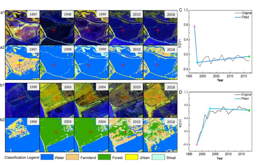
Remote Sens. 2019, 11, 1234                                                                           2 of 15

date, many studies have applied Landsat time-series analysis to long-term monitoring of cropland
change [12,13]. Such remote sensing time series can be used to separate long-term and short-term
land-use changes more reliably in highly resilient land systems. Zhe [14] provided a comprehensive
review of change detection approaches using Landsat time-series data, including the description of
frequencies, preprocessing, algorithms, and applications.
      Choosing a suitable algorithm is a critical step for conducting change detection [15].
Several change-detection techniques based on Landsat time series have been developed to be robust
against spectral variations arising from topography and phenology [16]. For example, Landsat-based
Detection of Trends in Disturbance and Recovery (LandTrendr) and Breaks For Additive Season
and Trend (BFAST) have been applied to monitor cropland change [17,18]. BFAST has been used to
investigate cropping systems and temporal paddy crop dynamics in Sidoarjo Regency, Indonesia,
and provide accurate and up-to-date information on agricultural land-use changes [19,20]. LandTrendr
can be used to identify cropland abandonment and re-cultivation based on annual time series of
cropland probabilities; it can also contribute to the identification of different smallholder cultivation
patterns [21,22].
      The above change-detection algorithms, and others such as Continuous Change Detection and
Classification (CCDC) [23] are subject to considerable computational time in data-preprocessing and
are themselves time-consuming. In order to reach to a broader research community, the LandTrendr
algorithm (https://emapr.github.io/LT-GEE/) was implemented on the Google Earth Engine (GEE)
platform, which provides full access to the Landsat archive and parallel processing to increase
computational speed [24]. Compared to previous change detection algorithms run on local
servers [25,26], LandTrendr in GEE detects cropland change more efficiently with the advantages of
cloud computing and offers an opportunity to map large-scale cropland change [27].
      Previous change assessment studies have focused on cropland abandonment and re-cultivation
and detecting changes in their cultivation patterns. Thus, cropland conversion to other land cover
classes in areas such as Dongting Lake in China has not received much attention. Using LandTrendr
with GEE support, we can observe the process of cropland conversion to lake or poplar trees and
its spatial and temporal characteristics efficiently, understanding this process can provide the policy
enlightenment for ecological conservation in Dongting Lake.
      Our overarching goal therefore was to use LandTrendr with Landsat time-series in GEE to detect
cropland change processes in the Dongting Lake area, we analyzed a conceptual model of the spectral
feature trajectories related to cropland conversion to lake or poplar cultivation. We also parameterized
the LandTrendr algorithm and tested it based on Landsat time-series data to track these changes,
then compared their spatial and temporal characteristics.

2. Materials and Methods

2.1. Study Area
      Dongting Lake (28◦ 420 –29◦ 380 N, 111◦ 520 –113◦ 080 E), located in the north part of Hunan Province,
is the second largest freshwater lake in China with an area of 2794.7 km2 [28]. We defined our study
area by administrative divisions in the lake’s surrounding area, including 20 counties (districts) in
Yueyang, Yiyang, and Changde (Figure 1). This area included reclamation zones outside the Dongting
Lake embankment with internal lakes used mainly for agricultural production; while the area within
the embankment included the outer lake (East Dongting Lake, South Dongting Lake, Hengling Lake,
and West Dongting Lake).
      There has been excessive reclamation of the lake for almost 100 years, resulting in serious ecological
degradation of the wetland ecosystem associated with the lake. Following the great Yangtze River flood
in 1998, the CFTL was launched to help restore the lake’s ecology and guide the area’s development
in a more benign direction. After the project was initiated, agricultural land focused on two change
patterns: conversions back to lake were implemented mainly around in the outer lake area to improve
Remote Sens. 2019, 11, 1234                                                                                                  3 of 15

ecological functions, while poplar trees cultivation was implemented primarily in part of the outer
lake for economic
     Remote Sens. 2019, benefits.
                        11, x FOR PEER REVIEW                                           3 of 16

      Figure 1. Geographic location and land cover map of the study area: (a) general location in China;
      (b) location  inGeographic
            Figure 1.  Hunan Province;
                                 location(c)
                                          and1997
                                               landland-use
                                                    cover mapclassification  (prior
                                                               of the study area: (a)to Converting
                                                                                      general locationFarmland   to Lake
                                                                                                       in China; (b)
      (CFTL)   implementation)
            location              from Google
                     in Hunan Province;  (c) 1997Earth   Engine
                                                  land-use       (GEE) imagery
                                                           classification (prior to (see SectionFarmland
                                                                                    Converting    2.3). Thetored  frames
                                                                                                               Lake
      show(CFTL)
             the location of the twofrom
                    implementation)   typical  CFTL
                                          Google      areas.
                                                   Earth Engine (GEE) imagery (see Section 2.3),. The red frames
            show the location of the two typical CFTL areas.
     Two typical CFTL areas (Figure 1), the Qingshan Polder (28◦ 510 N, 112◦ 120 E) with an area
of 11.1 km  2 and
          There    hasthebeen     excessive
                             Jicheng    polder    (29◦ 410 of
                                             reclamation   N, the  ◦ 560 for
                                                               112lake    E) almost
                                                                             with an 100area
                                                                                           years,      km2in
                                                                                                  resulting
                                                                                              of 33.7           serious
                                                                                                            , are   taken as
examples (Figure 2). The local government led its cropland conversion to natural lake after great
     ecological   degradation        of the  wetland   ecosystem   associated   with   the lake.  Following  the  1998 with
     Yangtze
Qingshan       River flood
           Polder,      aiming   in 1998, the CFTL
                                    to restore       was launched
                                                a wetland           to help restore
                                                              ecosystem.            the lake’s
                                                                             As a typical       ecology and guide
                                                                                             demonstration     areathefor the
     area’s development in a more benign direction. After the project was initiated, agricultural land
CFTL project, Qingshan developed a green aquatic culture that did not require fertilizer or feed for
     focused on two change patterns: conversions back to lake were implemented mainly around in the
recovery. At Jicheng Polder, many poplars were planted to form a plantation forest system, based on
     outer lake area to improve ecological functions, while poplar trees cultivation was implemented
the pattern  of in
     primarily    poplar
                     part ofcultivation     after
                                the outer lake forlocal  residents
                                                    economic         moved outside the village and abandoned the
                                                              benefits.
cropland.Two
           Poplartypical CFTL areas (Figure 1), the Qingshan Polder of
                       cultivation      can  alleviate  the tight supply        medicinal
                                                                             (28°51′N,       materials
                                                                                         112°12′E)       and
                                                                                                   with an    promote
                                                                                                           area  of 11.1 the
        Remote Sens. 2019, 11, x FOR PEER REVIEW                                                              4 of 16
development      of  a local    economy     [29].
     km and the Jicheng polder (29°41′N, 112°56′) with an area of 33.7 km , are taken as examples (Figure
        2                                                                            2

      2). The local government led its cropland conversion to natural lake after 1998 with Qingshan Polder,
      aiming to restore a wetland ecosystem. As a typical demonstration area for the CFTL project,
      Qingshan developed a green aquatic culture that did not require fertilizer or feed for recovery. At
      Jicheng Polder, many poplars were planted to form a plantation forest system, based on the pattern
      of poplar cultivation after local residents moved outside the village and abandoned the cropland.
      Poplar cultivation can alleviate the tight supply of medicinal materials and promote the development
      of a local economy [29].

      Figure 2.  Two2. examples
              Figure   Two examples areas  ofofeach
                                        areas   eachcropland    change
                                                     cropland change      pattern.
                                                                       pattern.       Corresponding
                                                                                Corresponding           photos
                                                                                                photos a1 and a2,a1b1 and a2,
              andbefore
      b1 and b2   b2 before
                         andand  after
                              after    CFTLare
                                    CFTL     arefrom
                                                 from google
                                                      googleearth
                                                              earthtoto
                                                                      demonstrate
                                                                        demonstratethe process of conversion
                                                                                        the process          to lake, to lake,
                                                                                                     of conversion
              poplar cultivation
      poplar cultivation         respectively.
                           respectively.       Figures
                                            Figures  a1a1and
                                                          and b1
                                                              b1 represent
                                                                 representthetheyears 19971997
                                                                                  years    and and
                                                                                               figures a2 anda2
                                                                                                    figures   b2 and
                                                                                                                  the b2 the
              years 2018. Field photographs c1 and c2 were collected in 2018.
      years 2018. Field photographs c1 and c2 were collected in 2018.
         2.2. Data Preparation
              We used the GEE platform’s full archive to build stacks of Surface Reflectance Tier 1 Landsat
         TM/ETM+/OLI images from 1998–2018 for use with LandTrendr (Table 1). In order to minimize
         variations caused by phenology or changes in solar geometry, a total of 320 images across three
         path/row numbers were acquired in the crop-growing season (June 1 to September 1) within the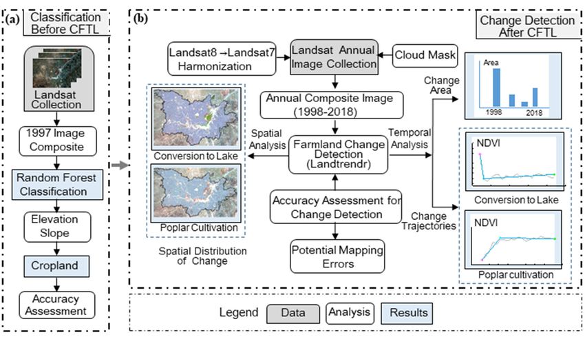
Remote Sens. 2019, 11, 1234                                                                                               4 of 15

2.2. Data Preparation
     We used the GEE platform’s full archive to build stacks of Surface Reflectance Tier 1 Landsat
TM/ETM+/OLI images from 1998–2018 for use with LandTrendr (Table 1). In order to minimize
variations caused by phenology or changes in solar geometry, a total of 320 images across three
path/row numbers were acquired in the crop-growing season (June 1 to September 1) within the whole
study period. As the Landsat 8/OLI has higher 12-bit radiometric resolution than the previous Landsat
7/ETM+, we applied statistical harmonization functions between the spectral values of both sensors to
normalize the reflectance [30]. Cloud, cloud shadow, and snow masks were produced from the Fmask
band. Finally, 21 annual composites from 320 images with minimal cloud cover were created using the
median reflectance values of the collection [31].

                                           Table 1. Datasets used in this study.

             Data                                    Description                                         Source
         Landsat5
                               Annual atmospherically corrected Surface Reflectance
         Landsat7                                                                          Pre-Collection 1 archive available
                               Collection from June to September, 1998–2018, for use
    Landsat8 (path/row:                                                                       from Google Earth Engine
                                                 with LandTrendr
  123/040,124/039,124/040)
                                    Advanced Spaceborne Thermal Emission and               ASTER Global Emissivity Dataset
            DEM                     Reflection Radiometer (ASTER) data used for            100 m V003 available from Google
                                             modification of classification                         Earth Engine
         Field survey          Inventory data within the study area, collected in 2018
                                                  Imagery used for
   High-resolution images                                                                             Google Earth
                                        validation of LandTrendr disturbance

        Remote Sens. 2019, 11, x FOR PEER REVIEW                                                                     5 of 16
2.3. Cropland Change Conceptual Model
        2.3. Cropland Change Conceptual Model
     Figure 3 presents the conceptual model of two cropland change patterns, from which the pattern
            Figure
of conversion       3 presents
                 to either  lakethe conceptual
                                  cover          model of
                                         over poplar         two cropland
                                                          cultivation     canchange
                                                                                be seen;patterns,  from which
                                                                                            this results         the pattern
                                                                                                           in a mixed    pattern
      of conversion    to either lake cover  over   poplar  cultivation    can  be  seen; this
of changes. To focus on the pattern of conversions to lakes, we removed poplar cultivations by  results in a  mixed  pattern
      of changes. To focus on the pattern of conversions to lakes, we removed poplar cultivations by
subtracting the superposition results of the two patterns using ArcGIS 10.4. Normalized Difference
      subtracting the superposition results of the two patterns using ArcGIS 10.4. Normalized Difference
Vegetation Index (NDVI) is a useful indicator for monitoring vegetation changes in agricultural
      Vegetation Index (NDVI) is a useful indicator for monitoring vegetation changes in agricultural
changechange
        areas areas
                [32,33],  so we
                      [32,33], so used  thisthis
                                  we used     to to
                                                  detect
                                                     detectcropland
                                                            cropland changes
                                                                        changes in   inthis
                                                                                        thisstudy.
                                                                                              study.WeWe    captured
                                                                                                         captured      as many
                                                                                                                    as many
examples
      examples of cropland conversion as possible to know how NDVI signatures would represent the the
            of cropland     conversion    as   possible    to  know     how     NDVI     signatures     would    represent
cropland  conversions.
      cropland             When
                  conversions.     cropland
                                 When  croplandis converted
                                                   is converted totolake,
                                                                      lake,the
                                                                             theinitially
                                                                                  initially higher   NDVIshould
                                                                                            higher NDVI       shoulddrop
                                                                                                                       dropto to a
much alower
        muchlevel
               lower(Figure     3a). When
                       level (Figure         cropland
                                     3a). When    croplandis is
                                                              converted
                                                                convertedto   to poplar   cultivation,
                                                                                 poplar cultivation,      NDVI
                                                                                                        NDVI       should
                                                                                                               should  dropdrop
      temporarily
temporarily          but recover
               but recover    to ato a higher
                                   higher       level
                                            level      than
                                                    than     before(Figure
                                                          before     (Figure 3b). These
                                                                                      Theseproposed
                                                                                               proposed  trajectories reflect
                                                                                                            trajectories  reflect
      occurrence,   duration,   and  magnitude     attributes,  which    respectively    express
occurrence, duration, and magnitude attributes, which respectively express the year of occurrence, the year  of occurrence,
      duration
duration  time, time,   andrange
                  and the    the range of NDVI
                                    of NDVI        variation
                                               variation       duringconversion.
                                                            during      conversion.

      FigureFigure   3. Conceptual
              3. Conceptual   modelsmodels    and several
                                      and several         examples
                                                   examples           for cropland
                                                             for cropland           conversion
                                                                            conversion            in the(a)CFTL:
                                                                                        in the CFTL:               (a)
                                                                                                            Normalized
             Normalized   Difference Vegetation Index (NDVI)  trajectory of conversion to lake; (b) NDVI   trajectory
      Difference Vegetation Index (NDVI) trajectory of conversion to lake; (b) NDVI trajectory of conversion
             of conversion
      to poplar            to poplar cultivation.
                 cultivation.

        2.4. Initial Land Cover Classification
            Prior to running the LandTrendr algorithm, we applied the Random Forest (RF) classifier [34] to
        pre-CFTL Landsat images in GEE to extract cropland areas (Figure 4a). First, Landsat images from
        1997 were used with the cloud and shadow masks to produce a cloud-free composite, from which
        the NDVI was calculated. Next, 250 training samples for each land-cover class were selected for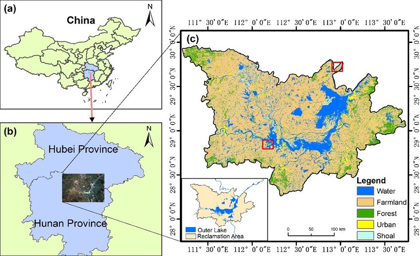
Remote Sens. 2019, 11, 1234                                                                                 5 of 15

2.4. Initial Land Cover Classification
     Prior to running the LandTrendr algorithm, we applied the Random Forest (RF) classifier [34] to
pre-CFTL Landsat images in GEE to extract cropland areas (Figure 4a). First, Landsat images from 1997
were used with the cloud and shadow masks to produce a cloud-free composite, from which the NDVI
was calculated. Next, 250 training samples for each land-cover class were selected for interpretation by
high-resolution imagery from Google Earth. As NDVI can be used to distinguish impervious surfaces,
bare soil, and water bodies from forest or croplands, this along with bands one through five, and seven
were used as feature inputs into the RF classifier with 20 trees. The resulting imagery was classified
into five land-cover categories: water, cropland, forest, urban, and shoal. Finally, elevation and slope
derived from GEE DEM data were used to modify the classification results for higher accuracy. In 1997,
Remote
the    Sens. land
    major    2019, 11, x FOR
                   cover     PEERwere
                           types REVIEW
                                      cropland and water (Figure 1c).                             6 of 16

      Figure 4.4. Methodological
      Figure      Methodologicalflowchart forfor
                                   flowchart  (a) pre-CFTL land-use
                                                  (a) pre-CFTL      classification
                                                                land-use           and (b)and
                                                                           classification  post-CFTL analysis
                                                                                               (b) post-CFTL
      of conversion  to lake and poplar cultivation.
      analysis of conversion to lake and poplar cultivation.

2.5. Monitoring Cropland Change with LandTrendr
2.5. Monitoring Cropland Change with LandTrendr
      We used the LandTrendr algorithm developed by Kennedy [35] to map and characterize post-CFTL
      We used the LandTrendr algorithm developed by Kennedy [35] to map and characterize post-
cropland changes (Figure 4b). The core of the LandTrendr algorithm is a temporal segmentation
CFTL cropland changes (Figure 4b). The core of the LandTrendr algorithm is a temporal
method used to capture both long-term gradual and short-term drastic changes; this approach can
segmentation method used to capture both long-term gradual and short-term drastic changes; this
monitor cropland change by analyzing the temporal-spectral trajectory of each pixel. The input for each
approach can monitor cropland change by analyzing the temporal-spectral trajectory of each pixel.
pixel is the annual time series of one spectral band or index, plus the date. The processing procedure
The input for each pixel is the annual time series of one spectral band or index, plus the date. The
for finding the best model involves removing noise-induced spikes (outliers), identifying potential
processing procedure for finding the best model involves removing noise-induced spikes (outliers),
vertices (breakpoints), fitting trajectories, and setting the optimal number of segments [23].
identifying potential vertices (breakpoints), fitting trajectories, and setting the optimal number of
      LandTrendr requires the setting of control parameters to ensure the quality of change detection,
segments [23].
so we analyzed examples of cropland conversion event, tested different combinations of parameter
      LandTrendr requires the setting of control parameters to ensure the quality of change detection,
values to determine the optimal combination of parameters. We also assessed the characteristics of
so we analyzed examples of cropland conversion event, tested different combinations of parameter
NDVI in the study area to exclude other change patterns in order to make LandTrendr more precise
values to determine the optimal combination of parameters. We also assessed the characteristics of
(Figure 5). NDVI before conversion ranged from 0.55–0.73, dropped sharply after conversion to lake
NDVI in the study area to exclude other change patterns in order to make LandTrendr more precise
(–0.25 to –0.16), and rose slightly after conversion to poplar cultivation (0.57–0.77). Therefore, for the
(Figure 5). NDVI before conversion ranged from 0.55–0.73, dropped sharply after conversion to lake
event of conversion to lake, we set the pre-lake-conversion NDVI to be >0.55 and the magnitude of
(–0.25 to –0.16), and rose slightly after conversion to poplar cultivation (0.57–0.77). Therefore, for the
NDVI decrease should be >0.71. While for the event of poplar cultivation, the pre-poplar-cultivation
event of conversion to lake, we set the pre-lake-conversion NDVI to be >0.55 and the magnitude of
NDVI > –0.25 and the magnitude of NDVI increase should be >0.73.
NDVI decrease should be >0.71. While for the event of poplar cultivation, the pre-poplar-cultivation
NDVI > –0.25 and the magnitude of NDVI increase should be >0.73.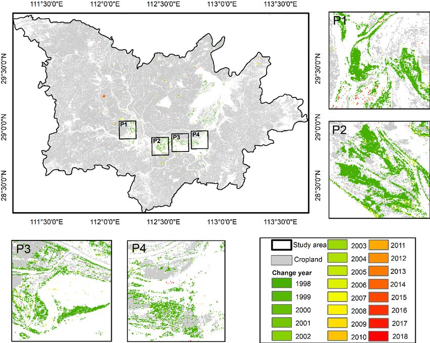
mote Sens. 2019, Remote
                  11, x Sens.
                         FOR2019,
                              PEER11, 1234
                                        REVIEW                                                                        6 of 15
                                                                                                                                7 of 1

                      Figure 5. NDVI range of cropland, conversion to lake, and conversion to poplar cultivation in the
     Figure 5. NDVI  range of cropland, conversion to lake, and conversion to poplar cultivation in the
                  study area.
     study area.
                  2.6. Accuracy Assessment and Validation
                      To assess the accuracy of the 1997 classification results, we selected validation sites different
6. Accuracy Assessment    and Validation
             from those used for training the classification algorithm, randomly generating 180 samples for each
                  land-cover class. We then produced a confusion matrix and estimates of overall accuracy, user accuracy,
    To assess and
               theproducer
                     accuracy        of the 1997 classification results, we selected validation sites differen
                              accuracy for each class following the methods defined by Foody [36] and Congalton and
 om those used    for[37].
              Green    training the classification algorithm, randomly generating 180 samples for eac
                   To assess the accuracy of the cropland conversions, during the study period we selected 300 pixels
 nd-cover class. We then produced a confusion matrix and estimates of overall accuracy, use
              representing conversion and another 300 pixels representing unchanged areas for each pattern in
ccuracy, and which
               producer        accuracy
                     the unchanged    pixels for
                                             were each
                                                  selectedclass
                                                            for thefollowing       the
                                                                    probability that theymethods     defined
                                                                                         were breaking           byeach
                                                                                                        points. For   Foody [36] an
ongalton andpixel,
                Green      [37]. inspected all 21 composite images and used high-spatial-resolution Google Earth
                    we visually
              imagery for further manual interpretation of land cover. We thus determined and recorded whether
    To assess and
               thewhen
                     accuracy        of the cropland conversions, during the study period we selected 30
                          (occurrence year) cropland conversion occurred at these pixels; if multiple changes occurred
 xels representing
             within aconversion         and
                        single pixel, only theanother      300 was
                                               greatest change   pixels
                                                                     usedrepresenting        unchanged areas for each patter
                                                                          in the accuracy assessment.
  which the unchanged
              3. Results       pixels were selected for the probability that they were breaking points. Fo
ach pixel, we visually inspected all 21 composite images and used high-spatial-resolution Goog
              3.1. Historical Change Process of Conversion Patterns
arth imagery for further manual interpretation of land cover. We thus determined and recorde
                   The disturbance map (Figure 6) was rendered as a gradient according to the occurrence years to
 hether and when
              present the(occurrence        year)
                            spatial and temporal     cropland
                                                 distribution        conversion
                                                               of conversion           occurred
                                                                              to lake during        at The
                                                                                             1998–2018.  these    pixels; if multip
                                                                                                             conversion
hanges occurred
             was within        a singlebutpixel,
                   widely dispersed          most only     theingreatest
                                                   prevalent                 change
                                                                   four regions:   Datongwas  used
                                                                                           Lake, WestinDongting
                                                                                                         the accuracy
                                                                                                                   Lake, assessmen
                  South Dongting Lake, and East Dongting Lake (Figure 6). Overall, 447.48 km2 of cropland was
                  converted to lake from 1998–2018 (Table 2). Annual change peaked in 1998 due to the CFTL project’s
 Results          initiation, after which conversion generally declined until 2012, when it began to increase again due to
                  new policies aimed at improving the protection and restoration of Dongting Lake.
1. Historical Change Process of Conversion Patterns
    The disturbance map (Figure 6) was rendered as a gradient according to the occurrence years t
resent the spatial and temporal distribution of conversion to lake during 1998-2018. The conversio
 as widely dispersed but most prevalent in four regions: Datong Lake, West Dongting Lake, Sout
ongting Lake, and East Dongting Lake (Figure 6). Overall, 447.48 km2 of cropland was converted t
ke from 1998–2018 (Table 2). Annual change peaked in 1998 due to the CFTL project’s initiation
 ter which conversion generally declined until 2012, when it began to increase again due to new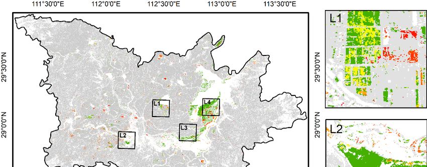
Remote Sens. 2019, 11, 1234 7 of 15
Remote Sens. 2019, 11, x FOR PEER REVIEW 8 of 16
Figure
Figure 6. Year
6. Year of conversion
of conversion fromcropland
from croplandto
to lake
lake with
withfour
fourareas
areasshown in in
shown detail: (L1)(L1)
detail: Datong Lake;Lake;
Datong
(L2) West Dongting Lake; (L3) South Dongting Lake; (L4) East Dongting Lake (scale of the four areas
(L2) West Dongting Lake; (L3) South Dongting Lake; (L4) East Dongting Lake (scale of the four areas is
is 1:130,000).
1:130,000).
TableTable 2. Yearly
2. Yearly change
change areaarea
for for
bothboth conversions
conversions from
from 1998toto2018
1998 2018by
byarea
areaand
and the
the conversion
conversion area
area per
year per
as ayear as a percentage
percentage of theconverted
of the total total converted
area area foryears.
for all all years .
Year Conversion to Lake Conversion to Poplar Cultivation
Year Conversion to Lake Conversion to2 Poplar Cultivation
Area (km2) Percentage Area (km ) Percentage
1998 Area (km2 )
258.98 Percentage
58.21% (km2 )
Area221.88 Percentage
44.39%
1999 1998 3.08
258.98 0.68%
58.21% 4.73
221.88 0.95%
44.39%
2000 1999 0.82
3.08 0.19%
0.68% 8.67
4.73 1.73%
0.95%
2001 2000 1.13
0.82 0.28%
0.19% 9.54
8.67 1.91%
1.73%
2002 2001 1.13
3.55 0.28%
0.87% 9.54
4.03 1.91%
0.81%
2003 2002 3.55
5.52 0.87%
1.24% 4.03
6.32 0.81%
1.26%
2004 2003 5.52
2.49 1.24%
0.54% 6.32
22.19 1.26%
4.44%
2005 2004 2.49
0.91 0.54%
0.21% 22.19
23.03 4.44%
4.61%
2006 2005 0.91
1.26 0.21%
0.30% 23.03
7.37 4.61%
1.47%
2007 2006 1.26
3.75 0.30%
0.84% 7.37
13.24 1.47%
2.65%
2008 2007 3.75
5.93 0.84%
1.33% 13.24
6.50 2.65%
1.30%
2009
2008 5.93
2.42
1.33%
0.52%
6.50
7.38
1.30%
1.48%
2009 2.42 0.52% 7.38 1.48%
2010 5.12 1.10% 7.94 1.59%
2010 5.12 1.10% 7.94 1.59%
2011 2.91 0.62% 19.53 3.91%
2011 2.91 0.62% 19.53 3.91%
2012 14.37 3.31% 8.02 1.61%
2012 14.37 3.31% 8.02 1.61%
2013 8.25 1.80% 39.00 7.80%
2013 8.25 1.80% 39.00 7.80%
2014 2014 51.38
51.38 11.07%
11.07% 34.58
34.58 6.92%
6.92%
2015 2015 13.83
13.83 3.13%
3.13% 7.77
7.77 1.55%
1.55%
2016 2016 31.76
31.76 6.76%
6.76% 9.01
9.01 1.80%
1.80%
2017 2017 14.62
14.62 3.47%
3.47% 19.97
19.97 4.00%
4.00%
2018 15.40 3.52% 19.19 3.84%
Total 447.48 100% 499.90 100%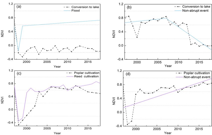
Remote Sens. 2019, 11, x FOR PEER REVIEW                                                               9 of 16

Remote Sens. 2019,
               201811, 1234       15.40            3.52%                  19.19                 3.84%               8 of 15

              Total              447.48             100%                 499.90                 100%

     FigureFigure
              7 was7 was
                      alsoalso rendered
                            rendered   asasa agradient
                                               gradientaccording
                                                         according to
                                                                    tothe
                                                                       theoccurrence
                                                                           occurrence years  to present
                                                                                         years          the spatial
                                                                                                 to present  the spatial
      and temporal
and temporal          distribution
                 distribution    of of poplarcultivation.
                                    poplar      cultivation. Conversion
                                                             Conversiontotopoplar
                                                                               poplarcultivation  waswas
                                                                                        cultivation   particularly
                                                                                                           particularly
      prominent
prominent         in West
             in West   andand   North
                             North     DongtingLake
                                     Dongting      Lake(P1,
                                                         (P1, and
                                                              and P2,
                                                                  P2,P3,
                                                                       P3,P4
                                                                           P4ininFigure 7).7).
                                                                                   Figure  TheThe
                                                                                                patterns of poplar
                                                                                                    patterns  of poplar
      cultivation events in inner lakes around Datong Lake did not follow the disturbance trends of the
cultivation events in inner lakes around Datong Lake did not follow the disturbance trends of the outer
      outer West and North Dongting Lake. The total area of poplar conversion was ~12% larger than that
West and North Dongting Lake. The total area of poplar conversion was ~12% larger than that of lake
      of lake conversion over the past 21 years (Table 2). Annual conversion spiked in two periods, 2004–
conversion   over the past 21 years (Table 2). Annual conversion spiked in two periods, 2004–2005 with
      2005 with disturbance rates which amounted to 4.44% and 4.61%, and 2013–2014 with disturbances
disturbance    ratesamounted
      rates which    which amounted
                               to 7.80% andto6.92%
                                               4.44%
                                                   . and 4.61%, and 2013–2014 with disturbances rates which
amounted to 7.80% and 6.92%.

           Figure
      Figure      7. Year
              7. Year  of of conversionfrom
                          conversion    from cropland
                                             croplandtoto
                                                        poplar cultivation
                                                          poplar           with four
                                                                   cultivation  withareas
                                                                                     fourshown
                                                                                          areas in detail: in
                                                                                                 shown     (P1)
                                                                                                              detail:
           West Dongting Lake; (P2); (P3); (P4) portions of North Dongting Lake (scale of the four areas is
      (P1) West Dongting Lake; (P2); (P3); (P4) portions of North Dongting Lake (scale of the four areas is
           1:130,000).
      1:130,000).
      3.2. Characterization
3.2. Characterization       of Two
                        of Two     ConversionPatterns
                                Conversion    Patterns
            NDVI spectral–temporal characteristics discriminated between two cropland change patterns
     NDVI spectral–temporal characteristics discriminated between two cropland change patterns
      (Figure 8). Of the pixels in which cropland was converted to lake, 82.4% showed a decline in NDVI
(Figure  8). Of the pixels in which cropland was converted to lake, 82.4% showed a decline in NDVI
      value between 0.70–0.90. The area near Datong Lake experienced a similar decline in NDVI between
value0.77–0.88
       between(Figure
                  0.70–0.90.  The area
                         8a), with  evennear  Datong
                                          higher NDVILake     experienced
                                                        declines  (0.99–1.10)aduring
                                                                                similarflooding
                                                                                          decline events
                                                                                                   in NDVI     between
                                                                                                           in East
0.77–0.88   (Figure   8a), with  even   higher  NDVI   declines    (0.99–1.10)    during    flooding
      Dongting Lake. The average duration of conversion to lake was 2.71 years; nearly 89.9% of relevantevents  in East
Dongting
      pixelsLake.
             rangedThe
                     fromaverage   duration
                           1–5 years         of conversion
                                     while 52.1%              to lake
                                                  were very short      was
                                                                    (two     2.71oryears;
                                                                          years            nearly8b).
                                                                                    less) (Figure   89.9%   of relevant
                                                                                                        Moreover,
pixelsEast
        ranged   fromLake
           Dongting    1–5 was
                            years  while 52.1%
                                dominated        were very
                                            by one-year       short[27].
                                                        durations    (two   years
                                                                          For everyorchange
                                                                                       less) (Figure   8b). Moreover,
                                                                                              pixel of conversion
      to poplar Lake
East Dongting    cultivation, we analyzed
                       was dominated         magnitudedurations
                                         by one-year    and duration
                                                                   [27]. characteristics
                                                                         For every change  of the poplar
                                                                                               pixel      growth to
                                                                                                      of conversion
      process  for the second  half of each LandTrendr   trajectory.  75.6%  of the  relevant  pixels
poplar cultivation, we analyzed magnitude and duration characteristics of the poplar growth process    showed   an
      increase in NDVI value between 0.73–1.02. Higher NDVI increases clustered at the centralized poplar
for the second half of each LandTrendr trajectory. 75.6% of the relevant pixels showed an increase in
      cultivation areas in North and West Dongting Lake (Figure 8c). The average duration of conversion
NDVI value between 0.73–1.02. Higher NDVI increases clustered at the centralized poplar cultivation
areas in North and West Dongting Lake (Figure 8c). The average duration of conversion to poplar
cultivation was 3.17 years, while the most common durations were 1 (23.5%) and 21 (17.1%) years.
Generally, longer change durations occurred in North Dongting Lake (Figure 8d) where the humid
climate was suitable for poplar growth [27].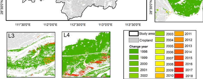
Remote Sens. 2019, 11, x FOR PEER REVIEW                                                               10 of 16

           to poplar cultivation was 3.17 years, while the most common durations were 1 (23.5%) and 21 (17.1%)
           years. Generally, longer change durations occurred in North Dongting Lake (Figure 8d) where the
Remote Sens.humid   climate
             2019, 11, 1234 was suitable for poplar growth [27].                                              9 of 15

      Figure 8. Figure  8. Magnitude
                 Magnitude             and duration
                               and duration          of conversion
                                             of conversion           from cropland
                                                            from cropland     to (a,b)tolake
                                                                                          (a,b)
                                                                                             andlake and
                                                                                                  (c,d)   (c,d) poplar
                                                                                                        poplar  cultivation
                cultivation in the Dongting Lake region. Close up looks for the prevalent  regions of two
      in the Dongting Lake region. Close up looks for the prevalent regions of two patterns are displayed.patterns are
                displayed.
3.3. Accuracy Assessment
           3.3. Accuracy Assessment
3.3.1. Accuracy Assessment for Initial Classification
           3.3.1. Accuracy Assessment for Initial Classification
     The confusion       matrix for the initially classified 1997 imagery (Table 3) indicated that the
              The confusion matrix for the initially classified 1997 imagery (Table 3) indicated that the overall
overall accuracy,   user    accuracy,and
         accuracy, user accuracy,       and   producer
                                           producer       accuracy
                                                     accuracy         forland-cover
                                                                for each  each land-cover     class
                                                                                      class were     were
                                                                                                 mostly         Three>80%.
                                                                                                            mostly
                                                                                                         >80%.
Three categories  (cropland,      forest, and  shoal)   were  most   frequently   misclassified.  Cropland
         categories (cropland, forest, and shoal) were most frequently misclassified. Cropland and forests     and  forests
         were  difficult  to distinguish  between  at the  30 m  Landsat  resolution, because forests
were difficult to distinguish between at the 30 m Landsat resolution, because forests are often small are often small
         and scattered
and scattered            in the study
               in the study     area. area.  In addition,
                                       In addition,       forests
                                                       forests andandshoals
                                                                       shoals were
                                                                              were often
                                                                                    oftenmisclassified likely
                                                                                            misclassified     because
                                                                                                           likely because
         other vegetation growing in shoals resemble forest in their spectral characteristics. Although the
other vegetation growing in shoals resemble forest in their spectral characteristics. Although the lower
         lower producer accuracies are indicative of errors related to the classification algorithm, the overall
producer accuracies are indicative of errors related to the classification algorithm, the overall accuracy
         accuracy was greater than 85% for each classification period, indicating the RF classifier was sufficient
was greater  thanstudy
         for this   85%area.
                           for each classification period, indicating the RF classifier was sufficient for this
study area.
                                      Table 3. Confusion matrix for the 1997 classified imagery.
                               Table 3. Confusion matrix for the 1997
                                                    Validation   Data classified imagery.
                      Class            Water      Cropland    Forest              Urban   Shoal       User Accuracy
                                                      Validation Data
              Class               Water        Cropland          Forest       Urban        Shoal         User Accuracy
           Water                   179              0              0                 0       0                100%
          Cropland                  1             153              24               10       30               70.2%
           Forest                   0              14             153                1       17               82.7%
           Urban                    0               3              1               168       1                97.1%
            Shoal                   0              10              2                 1      132
                                                                                                              91.0%
            Total                  180            180             180              180      180
      Producer Accuracy           99.4%          85.0%           85.0%            93.3%    73.3%
                                                      Overall accuracy = 87.2%.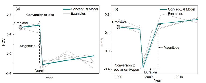
Shoal 0 10 2 1 132
91.0%
Total 180 180 180 180 180
Producer Accuracy 99.4% 85.0% 85.0% 93.3% 73.3%
Overall accuracy = 87.2%
Remote Sens. 2019, 11, 1234 10 of 15
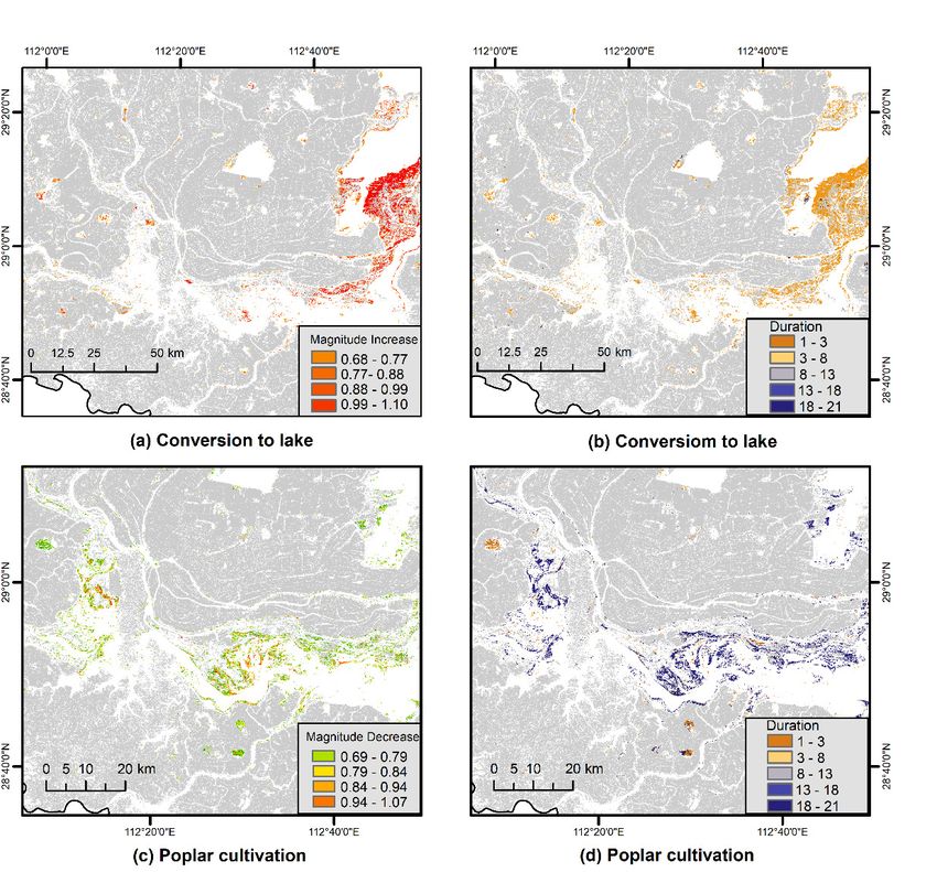
3.3.2. Accuracy Assessment for LandTrendr
The results
3.3.2. Accuracy of the segmentation
Assessment for LandTrendr and fitting algorithms suggest that both conversion patterns
were successfully captured by LandTrendr. Both accuracy assessments (Table 4) indicated high
The results
producer and of theaccuracies,
user segmentation and
with thefitting
overallalgorithms
accuracysuggest that both
of conversion to conversion
lake (87.0%) patterns were
being slightly
successfully captured by LandTrendr. Both accuracy assessments (Table 4) indicated
higher than conversion to poplar cultivation (83.8%). One typical area of each conversion type high producer
and user accuracies,
(Qingshan polderwith
and the overall
Jicheng accuracy
polder of conversion
described to lake
in Figure (87.0%)
2) was being
further slightlytohigher
studied thanthe
validate
conversion to poplar cultivation (83.8%). One typical area of each conversion type (Qingshan
algorithm, RF classification (Figure 9a2,b2) in specific years finished to help us better analyze the polder
and Jichengchanges.
relevant polder described in Figure
In the first 2) was 9a),
area (Figure further studied
original to validate
cropland wasthe algorithm,after
abandoned RF classification
the CFTL and
(Figure 9a2,b2) in specific years finished to help us better analyze the relevant
converted to lake from 1998 onward, a change conducive to wetland ecological recovery [28].changes. In the first area
In the
(Figure
second area (Figure 9b), cropland was abandoned before poplar planting prior to 2002 onward,
9a), original cropland was abandoned after the CFTL and converted to lake from 1998 but these
a change conducive
plantings to wetland
were decreasing byecological
2010. recovery [28]. In the second area (Figure 9b), cropland was
abandoned before poplar planting prior to 2002 but these plantings were decreasing by 2010.
Figure 9. Landsat spectral trajectories and LandTrendr fitted trajectories in typical areas (crosses
Figure 9. Landsat spectral trajectories and LandTrendr fitted trajectories in typical areas (crosses
indicate trajectory locations) for (a,C) conversion to lake and (b,D) conversion to poplar cultivation.
indicate trajectory locations) for (a,c) conversion to lake and (b,d) conversion to poplar cultivation.
Related imagery (a1,b1,bands 4–5–3) and corresponding Landsat classification results(a2,b2) are also
Related imagery (a1,b1,bands 4–5–3) and corresponding Landsat classification results(a2,b2) are also
shown at left.
shown at left.
Table 4. Accuracy
Table assessments
4. Accuracy forfor
assessments change detection
change in both
detection conversion
in both patterns.
conversion patterns.
Conversion
Conversion to lake
to Lake
Changed pixels
Changed Pixels Stable pixels
Stable Pixels Total Total User Accuracy
User Accuracy
Changed
Changedpixels
pixels 258
258 42 42 300 300 86.0% 86.0%
Stable
Stablepixels
pixels 36
36 264264 300 300 88.0% 88.0%
Total
Total 294
294 306306
Producer Accuracy 87.8 86.3% Overall 87.0%
Conversion to Poplar Cultivation
Changed Pixels Stable Pixels Total User Accuracy
Changed pixels 245 55 300 81.7%
Stable pixels 42 258 300 86.0%
Total 287 313
Producer Accuracy 85.4% 82.4% Overall 83.8%
Note: Stable pixels means areas where land cover was persistent throughout the time of the analysis (1998–2018).Remote Sens. 2019, 11, 1234 11 of 15
4. Discussion
4.1. Mapping Approach
LandTrendr in this study detected different spatial distribution characteristics accurately under
both conversion patterns. Conversion to lake detected most prevalent around Datong Lake, because of
the Government encouraged the improvement of water storage capacity of the inner lake by excavating
deep ponds near Datong Lake (L1 in Figure 6), while the East, South, and West Dongting Lake areas
(L2, L3, and L4 in Figure 6 respectively) have also undergone large-scale improvements to improve their
interconnectivity and improve the ecological function of Dongting Lake as a whole [38]. Conversion to
poplar cultivation was particularly prominent in West and North Dongting Lake due to raw material
supply bases set up in this regions to develop the local economy, resulting in large-scale poplar planting
in this district.
Using LandTrendr resulted in producer and user accuracies high enough to detecting different
spatial and temporal characteristics under both conversion patterns. Compare the user’s accuracy
between changed and stable pixels, the relatively low accuracy for changed pixels indicated that
commission errors did occur; we identified four types (Figure 10). First, errors can be caused by
transient change events like floods (such as the major flooding in 1998), which can lead to incorrect
classification as conversion to lake (Figure 10a). Second, non-abrupt conversion to lake, which occurs
when the NDVI signals are unstable, leads to advance or lag segments in the fitted trajectories
(Figure 10b). Third, reed plantings have the same NDVI fluctuation range as poplars and the two can
be difficult to distinguish (Figure 10c). Fourth, non-abrupt poplar cultivation events produce gradual
changes while the NDVI before or after the conversion have strong fluctuations (Figure 10d). In these
cases, the fitted trajectory does not reach the set p-value parameter (0.05), making the segmentation
of the LandTrendr return a straight line as a segment for whole trajectory. Despite these potential
errors, the high producer and user accuracies for both conversion patterns imply that the LandTrendr
approach
Remote Sens. used in xthis
2019, 11, FORresearch was robust.
PEER REVIEW 13 of 16
Figure 10. Four
Four types
types ofof commission
commission errors
errors possible
possible when
when assessing
assessing cropland
cropland conversion
conversion with
LandTrendr: (a) (a)transient
transientfloods misclassified
floods misclassifiedas as
conversion
conversionto lake; (b) non-abrupt
to lake; conversion
(b) non-abrupt to lake;
conversion to
(c) reed
lake; cultivation
(c) reed producing
cultivation producinga similar NDVI
a similar NDVI signal as as
signal poplar
poplarcultivation;
cultivation;(d)
(d)non-abrupt
non-abrupt poplar
poplar
cultivation. The
Thetypical
typicaltrajectory for for
trajectory eacheach
errorerror
(blue (blue
or purple solid line)
or purple andline)
solid real cropland
and realconversion
cropland
(black dotted
conversion line)dotted
(black were extracted from
line) were NDVI from
extracted series.NDVI series.
4.2. Benefits of Change Detection Using LandTrendr in GEE
Accurate information about the timing and extent of cropland change is crucial for
environmental assessment and policy making [39]. In contrast to analyzed cropland abandonment
and re-cultivation via LandTrendr [40], we used this approach to study cropland conversion to otherRemote Sens. 2019, 11, 1234 12 of 15
4.2. Benefits of Change Detection Using LandTrendr in GEE
Accurate information about the timing and extent of cropland change is crucial for environmental
assessment and policy making [39]. In contrast to analyzed cropland abandonment and re-cultivation
via LandTrendr [40], we used this approach to study cropland conversion to other land cover classes.
By using this temporal segmentation algorithm with a time series of Landsat data, we were able to map
the spatial and temporal characteristics of different cropland conversion type. One clear advantage
of Landsat is the availability of consistent data for over three decades, allowing long-term analyses.
Compared to multi-date change mapping, the Landsat time series used here allowed us to map more
deviations in detail [41].
Although change detection-related studies have seen a considerable amount of research using
LandTrendr using data on local servers [25,35,42], the algorithm is still limited by time-consuming
data management work. In contrast, there are a few advantages of LandTrendr with GEE support to
monitor cropland change. Firstly, images are mostly prepared and updated by Google for cropland
change analysis. Secondly, GEE had an increased speed and great advantages in terms of vast data
handling and management cost [43,44], after data processing, the actual LandTrendr computational
cost and time are also reduced. Moreover, implementation in GEE makes it available to a much broader
base of users for those lack the technical capacity, experience, or financial means.
4.3. Research Limitations
Vegetation indices have been regarded as better variables than individual spectral bands, in terms
of monitoring land cover change, because they can reduce the impacts of external factors such as
topography and atmosphere on the surface reflectance. Selecting suitable vegetation indices is critical for
successfully detecting cropland conversion in our study; different vegetation indices, such as Enhanced
Vegetation Index (EVI) [20] and NDVI [32,45], have been used for this purpose. Research shows
that NDVI distinguishes cropland change better than other indices [46,47], but there are still some
limitations to applying the LandTrendr algorithm with NDVI. One example is the disturbance caused
by other vegetation, such as the reeds in our study region that produced an NDVI signal similar to
poplar and thus influenced the detection result. It is unclear whether or not NDVI is the best index to
use for the Dongting Lake region; more research is needed to identify an optimum.
5. Conclusions
In this study, we showed the effectiveness of a trajectory-based change detection approach to
characterize two cropland change patterns in China’s Dongting Lake region. By using the LandTrendr
algorithm with Landsat imagery derived from the Google Earth Engine, we detected and mapped
the conversion of cropland to lake and poplar cultivation with overall accuracies of 87.0% and 83.8%,
respectively. Conversion to lake covered a wider range, mainly distributed in areas surrounding the
outer lake and Datong Lake, while conversion to poplar cultivation was more prevalent in North and
West Dongting Lake. Over the entire study period, almost 947.38 km2 of cropland was converted,
with poplar accounting for 52.42 km2 more than lake. Some differences were apparent between the two
conversion patterns when their spectral–temporal characteristics were compared. For lake conversion
pixels, 82.4% had a decline in NDVI value between 0.70–0.90, while 75.6% of poplar-conversion pixels
increased by 0.73–1.02. We also found a high proportion of short-duration (two years or less) pixels for
conversion to lake, while the average duration of poplar cultivation pixels was a bit longer. These results
can assist researchers and managers in better understanding the conversion processes over time in this
region while providing baseline information for assessing the environmental influences of cropland
conversion in the Dongting Lake region.
Author Contributions: Conceptualization, X.L. and L.Z.; Data curation, L.Z., L.W. and Y.T.; Formal analysis,
L.Z., L.W. and Y.T.; Methodology, L.Z. and Y.T.; Supervision, X.L.; Validation, and L.W.; Visualization, Y.M.;
Writing—Original Draft Preparation, L.Z.; Writing—Review & Editing, X.L., L.W. and Y.M.Remote Sens. 2019, 11, 1234 13 of 15
Funding: This research was funded by the National Natural Science Foundation of China under Grant 41871223
and the Fundamental Research Funds for the Central Universities under Grant 2652017116.
Acknowledgments: The authors would like to thank the anonymous reviewers and the editor for their constructive
comments and suggestions for this paper.
Conflicts of Interest: The authors declare no conflict of interest.
References
1. Xu, C.; Mcgowan, S.; Lei, X.; Zeng, L.; Yang, X. Effects of hydrological regulation and anthropogenic
pollutants on Dongting Lake in the Yangtze floodplain. Ecohydrology 2016, 9, 315–325.
2. Hereher, M.E. Environmental monitoring and change assessment of Toshka lakes in southern Egypt using
remote sensing. Environ. Earth Sci. 2015, 73, 3623–3632. [CrossRef]
3. Qi, S.H.; Brown, D.G.; Tian, Q.; Jiang, L.G.; Zhao, T.T.; Bergen, K.M. Inundation extent and flood frequency
mapping using LANDSAT imagery and digital elevation models. Mapp. Sci. Remote Sens. 2009, 46, 101–127.
[CrossRef]
4. Kraemer, R.; Prishchepov, A.V.; Müller, D.; Kuemmerle, T.; Radeloff, V.C.; Dara, A.; Terekhov, A.; Frühauf, M.
Long-term agricultural land-cover change and potential for cropland expansion in the former Virgin Lands
area of Kazakhstan. Environ. Res. Lett. 2015, 10, 054012. [CrossRef]
5. Woodcock, C.E.; Richard, A.; Martha, A.; Alan, B.; Robert, B.; Warren, C.; Feng, G.; Goward, S.N.; Dennis, H.;
Eileen, H. Free access to Landsat imagery. Science 2008, 320, 1011. [CrossRef] [PubMed]
6. Röder, A.; Stellmes, M.; Hill, J.; Kuemmerle, T.; Tsiourlis, G.M. Analysing land cover change using time
series analysis of Landsat data and geoinformation processing. A natural experiment in Northern Greece.
Proc. SPIE Int. Soc. Opt. Eng. 2008, 7104, 43–56.
7. Rogan, J.; Franklin, J.; Roberts, D.A. A comparison of methods for monitoring multitemporal vegetation
change using Thematic Mapper imagery. Remote Sens. Environ. 2002, 80, 143–156. [CrossRef]
8. Wohlfart, C.; Mack, B.; Liu, G.; Kuenzer, C. Multi-faceted land cover and land use change analyses in the
Yellow River Basin based on dense Landsat time series: Exemplary analysis in mining, agriculture, forest,
and urban areas. Appl. Geogr. 2017, 85, 73–88. [CrossRef]
9. Liao, C.; Feng, Z.; Peng, L.I.; Zhang, J. Monitoring the spatio-temporal dynamics of swidden agriculture and
fallow vegetation recovery using Landsat imagery in northern Laos. Acta Geogr. Sin. 2015, 25, 1218–1234.
[CrossRef]
10. Forkuor, G.; Conrad, C.; Thiel, M.; Zoungrana, B.; Tondoh, J. Multiscale Remote Sensing to Map the Spatial
Distribution and Extent of Cropland in the Sudanian Savanna of West Africa. Remote Sens. 2017, 9, 839.
[CrossRef]
11. Falkowski, M.J.; Manning, J.A. Parcel-based classification of agricultural crops via multitemporal Landsat
imagery for monitoring habitat availability of western burrowing owls in the Imperial Valley agro-ecosystem.
Can. J. Remote Sens. 2010, 36, 750–762. [CrossRef]
12. Justice, C.J. Landsat-derived cropland mask for Tanzania using 2010–2013 time series and decision tree
classifier methods. In Proceedings of the Agu Fall Meeting, College Park, MD, USA, 17 December 2015.
13. Xu, Y.; Yu, L.; Zhao, F.R.; Cai, X.; Zhao, J.; Lu, H.; Gong, P. Tracking annual cropland changes from 1984 to 2016
using time-series Landsat images with a change-detection and post-classification approach: Experiments
from three sites in Africa. Remote Sens. Environ. 2018, 218, 13–31. [CrossRef]
14. Zhe, Z. Change detection using landsat time series: A review of frequencies, preprocessing, algorithms,
and applications. Isprs J. Photogramm. Remote Sens. 2017, 130, 370–384. [CrossRef]
15. Lu, D.; Li, G.; Moran, E. Current situation and needs of change detection techniques. Int. J. Image Data Fusion
2014, 5, 13–38. [CrossRef]
16. Griffiths, P.; Kuemmerle, T.; Kennedy, R.E.; Abrudan, I.V.; Knorn, J.; Hostert, P. Using annual time-series
of Landsat images to assess the effects of forest restitution in post-socialist Romania. Remote Sens. Environ.
2012, 118, 199–214. [CrossRef]
17. Novo-Fernández, A.; Franks, S.; Wehenkel, C.; López-Serrano, P.M.; Molinier, M.; López-Sánchez, C.A.
Landsat time series analysis for temperate forest cover change detection in the Sierra Madre Occidental,
Durango, Mexico. Int. J. Appl. Earth Obs. Geoinf. 2018, 73, 230–244. [CrossRef]Remote Sens. 2019, 11, 1234 14 of 15
18. Verbesselt, J.; Herold, M.; Hyndman, R.; Zeileis, A.; Culvenor, D. A robust approach for phenological change
detection within satellite image time series. In Proceedings of the Analysis of Multi-Temporal Remote
Sensing Images, Trento, Italy, 12–14 July 2011.
19. Fatikhunnada, A.; Seminar, K.B.; Solahudin, M.; Buono, A. Optimization of Parallel K-means for Java Paddy
Mapping Using Time-series Satellite Imagery. Telkomnika 2018, 16, 1409–1415. [CrossRef]
20. Huang, K.; Tao, Z.; Xiang, Z. Extreme Drought-induced Trend Changes in MODIS EVI Time Series in Yunnan,
China. IOP Conf. Ser. Earth Environ. Sci. 2014, 17, 012070. [CrossRef]
21. Schneibel, A.; Stellmes, M.; Röder, A.; Frantz, D.; Kowalski, B.; Haß, E.; Hill, J. Assessment of spatio-temporal
changes of smallholder cultivation patterns in the Angolan Miombo belt using segmentation of Landsat time
series. Remote Sens. Environ. 2017, 195, 118–129. [CrossRef]
22. Dara, A.; Baumann, M.; Kuemmerle, T.; Pflugmacher, D.; Rabe, A.; Griffiths, P.; Hölzel, N.; Kamp, J.;
Freitag, M.; Hostert, P. Mapping the timing of cropland abandonment and recultivation in northern
Kazakhstan using annual Landsat time series. Remote Sens. Environ. 2018, 213, 49–60. [CrossRef]
23. Zhe, Z.; Woodcock, C.E. Continuous change detection and classification of land cover using all available
Landsat data. Remote Sens. Environ. 2014, 144, 152–171. [CrossRef]
24. Gorelick, N.; Hancher, M.; Dixon, M.; Ilyushchenko, S.; Thau, D.; Moore, R. Google Earth Engine:
Planetary-scale geospatial analysis for everyone. Remote Sens. Environ. 2017, 202, 18–27. [CrossRef]
25. Watts, L.M.; Laffan, S.W. Effectiveness of the BFAST algorithm for detecting vegetation response patterns in
a semi-arid region. Remote Sens. Environ. 2014, 154, 234–245. [CrossRef]
26. Li, Z.; Wu, W.; Liu, X.; Fath, B.D.; Sun, H.; Liu, X.; Xiao, X.; Cao, J. Land use/cover change and regional climate
change in an arid grassland ecosystem of Inner Mongolia, China. Ecol. Model. 2017, 353, 86–94. [CrossRef]
27. Shelestov, A.; Lavreniuk, M.; Kussul, N.; Novikov, A.; Skakun, S. Exploring Google Earth Engine Platform
for Big Data Processing: Classification of Multi-Temporal Satellite Imagery for Crop Mapping. Front. Earth
Sci. 2017, 5, 17. [CrossRef]
28. Hu, Y.; Huang, J.; Yun, D.; Han, P.; Wei, H. Monitoring Spatial and Temporal Dynamics of Flood Regimes
and Their Relation to Wetland Landscape Patterns in Dongting Lake from MODIS Time-Series Imagery.
Remote Sens. 2015, 7, 7494–7520. [CrossRef]
29. Li, Y.; Chen, X.; Xie, Y.; Li, X.; Li, F.; Hou, Z. Effects of young poplar plantations on understory plant diversity
in the Dongting Lake wetlands, China. Sci. Rep. 2014, 4, 6339. [CrossRef]
30. Roy, D.P.; Kovalskyy, V.; Zhang, H.K.; Vermote, E.F.; Yan, L.; Kumar, S.S.; Egorov, A. Characterization
of Landsat-7 to Landsat-8 reflective wavelength and normalized difference vegetation index continuity.
Remote Sens. Environ. 2016, 185, 57–70. [CrossRef]
31. Simonetti, D.; Simonetti, E.; Szantoi, Z.; Lupi, A.; Eva, H.D. First Results From the Phenology-Based Synthesis
Classifier Using Landsat 8 Imagery. IEEE Geosci. Remote Sens. Lett. 2015, 12, 1496–1500. [CrossRef]
32. Zhang, Y.; Gao, J.; Liu, L.; Wang, Z.; Ding, M.; Yang, X. NDVI-based vegetation changes and their responses
to climate change from 1982 to 2011: A case study in the Koshi River Basin in the middle Himalayas.
Glob. Planet. Chang. 2013, 108, 139–148. [CrossRef]
33. Bai, J.J.; Bai, J.T.; Wang, L. Spatio-temporal Change of Vegetation NDVI and Its Relations with Regional
Climate in Northern Shaanxi Province in 2000–2010. Sci. Geogr. Sin. 2014, 34, 882–888.
34. Mainknorn, M.; Cohen, W.B.; Kennedy, R.E.; Grodzki, W.; Pflugmacher, D.; Griffiths, P.; Hostert, P.
Monitoring coniferous forest biomass change using a Landsat trajectory-based approach. Remote Sens.
Environ. 2013, 139, 277–290. [CrossRef]
35. Kennedy, R.E.; Yang, Z.; Cohen, W.B. Detecting trends in forest disturbance and recovery using yearly
Landsat time series: 1. LandTrendr—Temporal segmentation algorithms. Remote Sens. Environ. 2010, 114,
2897–2910. [CrossRef]
36. Foody, G.M. Status of land cover classification accuracy assessment. Remote Sens. Environ. 2002, 80, 185–201.
[CrossRef]
37. Congalton, R.G.; Green, K. Practical look at the sources of confusion in error matrix generation.
Photogramm. Eng. Remote Sens. 1993, 59, 641–644.
38. Bo, Y.; Zeng, F.; Yuan, M.; Li, D.; Qiu, Y.; Li, J. Measurement of Dongting Lake Area Based on Visual
Interpretation of Polders. Proced. Environ. Sci. 2011, 10, 2684–2689.
39. Zhang, P.L.; Bo, L.R.; Chao, J. An Object-based Basic Farmland Change Detection Using High Spatial
Resolution Image and GIS Data of Land Use Planning. Key Eng. Mater. 2012, 500, 492–499. [CrossRef]Remote Sens. 2019, 11, 1234 15 of 15
40. Yin, H.; Prishchepov, A.V.; Kuemmerle, T.; Bleyhl, B.; Buchner, J.; Radeloff, V.C. Mapping agricultural land
abandonment from spatial and temporal segmentation of Landsat time series. Remote Sens. Environ. 2018,
210, 12–24. [CrossRef]
41. Schmidt, M.; Pringle, M.; Devadas, R.; Denham, R.; Dan, T. A Framework for Large-Area Mapping of Past
and Present Cropping Activity Using Seasonal Landsat Images and Time Series Metrics. Remote Sens. 2016,
8, 312. [CrossRef]
42. Schwantes, A.M.; Swenson, J.J.; Jackson, R.B. Quantifying drought-induced tree mortality in the open canopy
woodlands of central Texas. Remote Sens. Environ. 2016, 181, 54–64. [CrossRef]
43. Long, T.; Zhang, Z.; He, G.; Jiao, W.; Tang, C.; Wu, B.; Zhang, X.; Wang, G.; Yin, R. 30 m resolution Global
Annual Burned Area Mapping based on Landsat images and Google Earth Engine. Remote Sens. 2019, 11, 489.
[CrossRef]
44. Dong, J.; Xiao, X.; Menarguez, M.A.; Zhang, G.; Qin, Y.; Thau, D.; Biradar, C.; Iii, B.M. Mapping paddy rice
planting area in northeastern Asia with Landsat 8 images, phenology-based algorithm and Google Earth
Engine. Remote Sens. Environ. 2016, 185, 142–154. [CrossRef] [PubMed]
45. Shrestha, R.; Di, L.; Yu, E.G.; Kang, L.; Shao, Y.Z.; Bai, Y.Q. Regression model to estimate flood impact on
corn yield using MODIS NDVI and USDA cropland data layer. J. Integr. Agric. 2017, 16, 398–407. [CrossRef]
46. Tian, H.; Wu, M.; Wang, L.; Niu, Z. Mapping Early, Middle and Late Rice Extent Using Sentinel-1A and
Landsat-8 Data in the Poyang Lake Plain, China. Sensors 2018, 18, 185. [CrossRef]
47. Tong, X.; Brandt, M.; Hiernaux, P.; Herrmann, S.M.; Feng, T.; Prishchepov, A.V.; Fensholt, R. Revisiting the
coupling between NDVI trends and cropland changes in the Sahel drylands: A case study in western Niger.
Remote Sens. Environ. 2017, 191, 286–296. [CrossRef]
© 2019 by the authors. Licensee MDPI, Basel, Switzerland. This article is an open access
article distributed under the terms and conditions of the Creative Commons Attribution
(CC BY) license (http://creativecommons.org/licenses/by/4.0/).You can also read