RAQ-A Random Forest Approach for Predicting Air Quality in Urban Sensing Systems
←
→
Page content transcription
If your browser does not render page correctly, please read the page content below
sensors
Article
RAQ–A Random Forest Approach for Predicting Air
Quality in Urban Sensing Systems
Ruiyun Yu 1, *, Yu Yang 2 , Leyou Yang 1 , Guangjie Han 3 and Oguti Ann Move 1
 Received: 30 September 2015; Accepted: 7 January 2016; Published: 11 January 2016
 Academic Editor: Leonhard M. Reindl
 1   Software College, Northeastern University, Shenyang 110819, China; yangleyou@163.com (L.Y.);
     annmove@swc.neu.edu.cn (O.A.M.)
 2   Department of Computer Science, Rutgers University, New Brunswick, NJ 08854, USA;
     yangyu.9415@rutgers.edu
 3   Department of Internet of Things Engineering, Hohai University, Changzhou 213022, China;
     hanguangjie@gmail.com
 *   Correspondence: yury@mail.neu.edu.cn; Tel.: +86-24-8368-0515; Fax: +86-24-8368-0522

 Abstract: Air quality information such as the concentration of PM2.5 is of great significance for human
 health and city management. It affects the way of traveling, urban planning, government policies
 and so on. However, in major cities there is typically only a limited number of air quality monitoring
 stations. In the meantime, air quality varies in the urban areas and there can be large differences,
 even between closely neighboring regions. In this paper, a random forest approach for predicting air
 quality (RAQ) is proposed for urban sensing systems. The data generated by urban sensing includes
 meteorology data, road information, real-time traffic status and point of interest (POI) distribution.
 The random forest algorithm is exploited for data training and prediction. The performance of RAQ
 is evaluated with real city data. Compared with three other algorithms, this approach achieves better
 prediction precision. Exciting results are observed from the experiments that the air quality can be
 inferred with amazingly high accuracy from the data which are obtained from urban sensing.

 Keywords: air quality prediction; random forest; point of interest; traffic

1. Introduction
      As urbanization leads to urban community growth, the transportation infrastructure dependent
on fossil fuels also expands consequently [1]. The popularity in vehicle use gives rise to an increase
in traffic related pollutant emissions. Urban air pollution is a major problem in both developed and
developing countries, as atmospheric pollutants have a great effect on human health. Numerous
illnesses such as lung cancer may be caused by various atmospheric pollutants [2]. In addition, some
other serious environmental problems can also result from air pollution, such as acid rain and the
greenhouse gas effect. For example, SO2 and NO2 are the main causes of acid rain [3], while CO2 and
N2 O are the main reasons for the greenhouse gas effect [3]. Recently, especially in China, environmental
problems have become a major concern in big cities such as Beijing and Shanghai, where the primary
sources of pollutants include exhaust emissions from Beijing's more than five million motor vehicles,
coal burning in neighboring regions, dust storms from the north and local construction dust [4].
A particularly severe smog engulfed the Beijing for weeks in early 2013, elevating public awareness to
unprecedented levels and prompting the government to roll out emergency measures [4]. Air pollution
monitoring is thus becoming more and more significant. Real-time air quality information, such as
the concentration of PM2.5 , PM10 and NO2 , is an important aspect for pollution management and
protecting human beings from damages caused by air pollutants. Considering the significance of
air quality, governments take measures to monitor it through establishing air quality monitoring

Sensors 2016, 16, 86; doi:10.3390/s16010086                                    www.mdpi.com/journal/sensors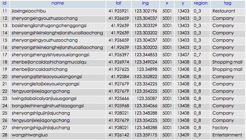
Sensors 2016, 16, 86 2 of 18
Sensors 2016, 16, 86 2 of 18
Sensors 2016, 16, 86 2 of 18
through establishing air quality monitoring stations. However, because of the high expense to start
stations. However, because of the high expense to start up and maintain these facilities, there are not
up and establishing
through maintain these facilities,
air quality there are stations.
monitoring not sufficient
However,stations in cities.
because of theForhighexample,
expenseFigureto start1
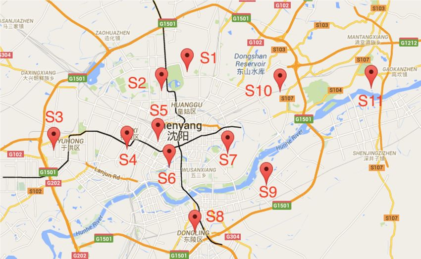
sufficient stations in cities. For example, Figure 1 shows the Google Map of Shenyang City. The red
shows
up and the Googlethese
maintain Mapfacilities,
of Shenyang thereCity. Thesufficient
are not red pins stations
represent in the 11 For
cities. air quality
example, monitoring
Figure 1
pins represent
stations. the 11
Among air quality
them, monitoring stations. Among them,
S8 areS1 is locatedthe in roofs
a college; S2, S3, S4,
shows the Google MapS1ofis Shenyang
located in aCity.
college;
TheS2,redS3, S4, S6,
pins represent located
the 11 on air quality of buildings;
monitoring
S6,stations.
S8 are
S5, S9 arelocated on
located
Among the
along
them, roofs
S1roads; of buildings;
S10 in
is located S5,
is alocated S9 are
college;inS2, located
a park;
S3, S4,S11 along
S6, is roads;
S8located
are located S10
nearon is located
factories.
the roofsThese in a park;11S11
only
of buildings;
is S5,
located
stations near
S9 arethat factories.
coveralong
located These
moreroads; only
than S10 11 stations
threeis thousand that
located insquare cover more
a park;kilometers than three thousand
of downtown
S11 is located near factories. square
areaThese kilometers
in Shenyang.
only 11
of stations
downtown
Another area
example inis Shenyang.
to compare Another
London example
and is
Beijing. to compare
The area of London
Beijing
that cover more than three thousand square kilometers of downtown area in Shenyang. and
is 10 Beijing.
times The
bigger area
than of
Beijing is 10
London but
Another times bigger
the number
example than London
of monitoring
is to compare Londonbut the number
stations of monitoring
is less than
and Beijing. one fourth
The area stations is
of London’s
of Beijing less
is 10 times than one
[5]. bigger fourth
than of
One station
London’s
can only[5].
London but One
monitor station
an areacan
the number only monitor
ofofmonitoring
limited size, an area
therefore
stations of limited
precise
is less thanair size,
one therefore
quality
fourth reports precise
for many
of London’s air
[5]. quality
areas reports
cannot
One station
forcan
many
be onlyareas
generated. cannot
monitor be generated.
an area of limited size, therefore precise air quality reports for many areas cannot
be generated.
Figure1.1.Monitoring
Figure Monitoring station
station locations
locations in
in Shenyang
Shenyangcity
city(China).
(China).
Figure 1. Monitoring station locations in Shenyang city (China).
Figure 2a shows samples of the AQI data of 10 stations in different locations. The x-axis denotes
theFigure
Figure2a2ashows
different showssamples
stations and theof
samples the
the AQI
y-axis
of data
denotes
AQI of 10
data AQI.
of 10 stations
stations
Three barsinindifferent
different
in locations.
colorslocations.
denote the
TheThe
AQI x-axis denotes
at different
x-axis denotes
thethedifferent
times. stations
As demonstrated
different and the
stations andinthe y-axis
Figure
y-axis denotes
2a,denotesAQI.
stationsAQI. Three bars
at different
Three bars in colors
locations
in colors denote
can denote the
differ athe AQI
lot AQIat different
at theatsame times.
time
different
Astimes.
demonstrated
such in on
Figure
asAsS7demonstrated
and S8 in2a,
6 May stations
2015
Figure [6]. at
2a, Airdifferent
quality
stations locations
on continuous
at different can differ
locations twocan a lot
days at the
can
differ also same
a lotdisplay
at the timebigsuch
same jumps
timeas S7
andsuchS8 on
such as 6
as S7
AQIMay
and 2015
atS8
S3on [6].
which Air
6 May quality
raised
2015from on continuous
55 to
[6]. Air 408 inonthe
quality two days can
morning between
continuous also display
two days6can May big
2015
also jumps
and 7big
display such
May as
2015
jumps AQI
at such
S3 which
[6]. Figure
as AQI2braised from
shows
at S3 which55
the to 408
waysfrom
raised in the
in whichmorning between
air inquality
55 to 408 6
changes
the morning May 2015 and 7
follow 6different
between May
May 2015rules 2015 [6].
and 7inMay Figure
2015 2b
different
shows
[6]. the ways
locations.
Figure For in whichthe
2b example,
shows airways
no quality
matter changes
inwhether follow
which stations
air different
are
quality shortrules
achanges distancein different
follow apart locations.
like
different S5 and in
rules For
S6 or example,
a long
different
distance
nolocations. like
ForS5
matter whether and
example,S10,nothey
stations are ashowed
matter short different
distance
whether changes
apart
stations arelike between
S5 and
a short points
S6
distance in
or aapart
longtime.
distance
like S5 andlike S5aand
S6 or longS10,
distance like S5 and S10, they showed
they showed different changes between points in time. different changes between points in time.
5-4 14:00 AQI 5-5 8:00 AQI 5-6 8:00 AQI S6 S5 S10
200 5-4 14:00 AQI 5-5 8:00 AQI 5-6 8:00 AQI 162.5 S6 S5 S10
200
160 162.5
130
160
120 130
97.5
AQIAQI
AQIAQI
120
80 97.5
65
80
40 65
32.5
400
32.50
S1 S2 S3 S4 S5 S6 S7 S8 S9 S10
0
0 0:00 4:00 8:00 0:00 16:00 20:00
S1 S2 S3 S4station
S5 S6 codeS7 S8 S9 S10
0:00 4:00 8:00time
0:00 16:00 20:00
station code
(a) time
(b)
(a) (b)
Figure 2. (a) AQI Samples in Shenyang; (b) AQI Trend on 12 May 2015 in Shenyang.
Figure2.2.(a)
Figure (a)AQI
AQISamples
Samples in
in Shenyang;
Shenyang;(b)
(b)AQI
AQITrend
Trendon
on1212May
May2015
2015inin
Shenyang.
Shenyang.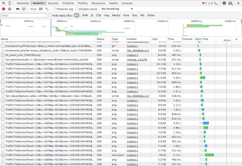
Sensors 2016, 16, 86                                                                               3 of 18

      It is hard to reflect these changes in a general function which can be applied to all the locations,
therefore, we cannot come up with a general formula to predict the air quality in a certain time slot.
Therefore, how to infer the air quality in the blank areas is a challenging and meaningful topic. In this
paper, we come up with an algorithm to infer the air quality indications throughout the city. In an
urban sensing system, an algorithm (RAQ) based on a random forest concept is proposed to predict
the urban area air quality through the use of historical air quality data, meteorology data, historical
traffic and road status as well as POI distribution information. These data are collected from all kinds
of urban sensors such as weather monitoring stations. This method hides all these kinds of inaccessible
factors in the traditional mathematic models. In practical applications, we cannot take all the factors
such as vehicle emissions and factory emissions into count, as it is hard to get accurate data about these
factors. This kind of replacement is not only good for the computation but also good for increased
prediction accuracy. At the same time, all the features used in this paper are much cheaper than the
accurate measured data from monitoring stations. No equipment cost is required in this approach.
As for the accuracy, this algorithm performs better than some other classical ones and the overall
results can provide meaningful references to citizens. Regarding the scalability and expansibility, more
possible related features such as human mobility can be input into this algorithm without significant
changes. The algorithm itself is also robust enough for even higher dimensions.
      The remainder of this paper is organized as follow: Section 2 presents related work. The problem
description and formulation are presented in Section 3. In Section 4, the system framework and the
RAQ algorithm is proposed. Extensive experiments are implemented in Section 5. We conclude and
outline the directions for future work in Section 6.

2. Related Work
      In the past decades, many studies on air quality inference have been done using approaches such
as dispersion models, satellite remote sensing and wireless sensor networks. Air pollution dispersion
models are tools that use a mathematical model such as the Box model [7], Gaussian model [8],
Lagrangian model [9], Eularian model [10], SLAB model [11] or some mixed models. to simulate
how air pollution disperses in the atmosphere. The classical dispersion models are mainly functions
of meteorology, traffic volumes, building distributions and so on. These models depend mainly on
experience and the parameters above to simulate the pollution dispersion, but some other potential
factors are not taken into consideration such as human mobility and concentrations. In the meantime,
dispersion models depend on access to relatively accurate data, such as the strength of pollutant
sources, wind speed, traffic emissions and so on, which accuracy cannot be guaranteed in certain
conditions. For example, wind speed may vary a lot in different regions because of the obstructions of
buildings, and their roles in determining the modified wind circulation between and over structures.
Accurate traffic emissions are also hard to obtain. We can only estimate the value according to the fuel
consumption and distances travelled.
      Satellite remote sensing technology is another possible way to monitor air quality. Research has
developed quickly using satellites to monitor air conditions in the past decades. For example, Liu et al.
came up with an approach using satellite remote sensing technology to test the thickness of PM2.5
on the ground [12]. Similarly, Martin et al. came up with a way of using satellite remote sensing
technology to test some ground air pollutants, including CO, NO, SO2 and so on [13]. Pawan et al. used
this technology to evaluate the air conditions of every city [14]. These methods mainly use satellite
remote sensing technology to directly measure the concentration of certain air pollutants by analyzing
the images obtained by the satellites to estimate the concentrations of air pollutants. However, many
air quality managers are not yet taking full advantage of satellite data for their applications because
of the challenges associated with accessing, processing, and properly interpreting observational data.
That is, a certain degree of technical skill is required on the part of the data end-user, which is often
problematic for organizations with limited resources [15].
Sensors 2016, 16, 86                                                                             4 of 18

     Sensor networks have also been studied extensively because of their broad applicability and
enormous application potential in areas such the environmental monitoring field. A Wireless Sensor
Network Air Pollution Monitor System (WAPMS) was deployed on the island of Mauritius for
monitoring air quality [16]; distributed infrastructure-based wireless sensor networks and grid
computing is also used for monitoring the air quality of London [17]. Rajasegarar et al. also used
wireless sensor networks to monitor air pollutants [18]. However, sensor networks require a large
number of sensor devices, and can only be deployed in a small range, such as indoors and in small areas.
For a city and other large areas, if using cheap sensors with single function, we cannot get information
about all kinds of air pollutants. If using sensors with complex functions such as monitoring stations,
infrastructure construction and maintenance costs make it difficult to promote wireless sensor networks
for a wide usage range. It is the same reason which limits the number of stations in cities of China.
     Besides all the methods above, participatory sensing is also an important approach for air quality
prediction. With the popularity of smart devices, participatory sensing and crowdsourcing has
been a hot topic of discussion in recent years. People see unlimited possibilities in smart devices.
A personalized mobile sensing system (MAQS) was proposed for indoor air quality monitoring [19];
a system based on smart phones and monitoring sensors has also been used to monitor outdoor
air quality [20]; noise pollution is also monitored using mobile phones [21]. Sivaraman et al. used
a participatory sensor system to monitor air pollutants in Sydney (Australia) [22]. However, most
current smartphones does not carry air pollutant sensors, so the sensing devices required for the
system need external sensing modules which leads to extra costs. Besides the high expense, user
participation and the accuracy of the data are problems that remain to be solved.
     Recently, urban computing has been one of the ways to solve problems in cities. Yuan Jing et al.
proposed an algorithm to infer the functional areas of cities by using trajectories [23]; Zheng et al.
made use of the city daily data to infer urban air quality [24,25]. However, similarly, urban computing
also requires pre-installed urban sensors such as GPS devices. For instance, when inferring the air
quality, Zheng made use of months of data collected from the GPS installed in taxis in Beijing. This
is an important limitation that prevents the promotion of this approach because in most cities we
cannot access the GPS information of taxis. Spatiotemporal data analysis is also an important aspect
for air quality prediction. Chen et al. established a spatiotemporal data framework named BigSmog to
provide China smog analysis [26]. Zhu et al. proposed Granger-causality-based air quality estimation
with heterogeneous spatiotemporal data [27]. Some other studies [28,29] also analyzed spatiotemporal
data to generate air pollutant distributions.

3. Problem Description and Definition

3.1. Definition

3.1.1. Air Quality Index
      An air quality index (AQI) is a number used by government agencies to communicate to the
public how polluted the air is currently or how polluted it is forecasted to become [30]. As the AQI
increases, an increasingly large percentage of the population is likely to be exposed, and people might
experience increasingly severe health effects. Different countries have their own air quality indices,
corresponding to different national air quality standards. In this paper, we use the standard of China,
where the AQI is based on the levels of six atmospheric gases, namely sulfur dioxide (SO2 ), nitrogen
dioxide (NO2 ), suspended particulates smaller than 10 µm in aerodynamic diameter (PM10 ), suspended
particulates smaller than 2.5 µm in aerodynamic diameter (PM2.5 ), carbon monoxide (CO), and ozone
(O3 ), measured at the monitoring stations throughout each city [31]. The AQI value is calculated per
hour according to a formula published by China’s Ministry of Environmental Protection [31]. AQI is
the maximum value of I AQI p which is a reference value of one air pollutant p:

                           AQI “ max tI AQI1 , I AQI2 , I AQI3 , . . . , I AQIn u                    (1)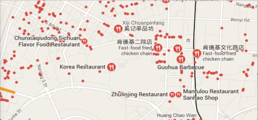
entration limit which can be checked in the reference table from the paper [31],                                                is the
e of the concentration limit which can be checked in the reference table from [31],                                                  i
esponding value of                   in the same reference table,                             is also the corresponding val
              Sensors 2016, 16, 86                                                                                 5 of 18
  in the reference       table. Table 1 shows the relationship between AQI values                                        and air pollu
 s which are marked by different colors.             I AQIH ´In     this
                                                                I AQI L `
                                                                           way, air˘     quality prediction can be treated
                                                               i           o
                                          I AQI p “                       C p ´ BPL ` I AQIL                           (2)
 ification problem so that we only need                 BPHto´ BP
                                                               i match
                                                                   L o      the air quality index to different classific
                                                                                          o     o

 s in Table 1.where
               TheCsix        levels
                        p is mass      in Table
                                   concentration    1 of
                                                 value  represent       sixp,AQI
                                                          the air pollutant    BPH islevels.
                                                                                      the high value of the concentration
                                                                                      i
                  limit which can be checked in the reference table from the paper [31], BPLo is the low value of the
                  concentration limit which can be checked in the reference table from [31], I AQIHi is the corresponding
                                                   Table
                  value of BPHi in the same reference        1. AQI
                                                          table, I AQILclassification.
                                                                        o is also the corresponding value of BPLo in the
                  reference table. Table 1 shows the relationship between AQI values and air pollution levels which are
                                                   AQI
                  marked by different colors. In this            Air Pollution
                                                      way, air quality prediction canLevel
                                                                                      be treated as a classification problem
                  so that we only need to match the air quality index to different classification levels in Table 1. The six
                                                   0–50
                  levels in Table 1 represent six AQI levels.
                                                                         Excellent
                                                51–100                   Good
                                                        Table 1. AQI classification.
                                                101–150           Lightly Polluted
                                                151–200
                                                     AQI      Moderately         Polluted
                                                                     Air Pollution   Level
                                                201–300
                                                     0–50        Heavily      Polluted
                                                                           Excellent
                                                    51–100                   Good
                                                 300+
                                                   101–150       Severely
                                                                       LightlyPolluted
                                                                                Polluted
                                                     151–200             Moderately Polluted
                                                     201–300              Heavily Polluted
. Traffic Congestion Status                           300+                Severely Polluted

 Traffic Congestion
             3.1.2. Traffic Status
                            Congestion(TCS)
                                       Status describes the traffic conditions on a certain road. Diff

 s denote differentTraffic Congestion
                        levels        Status (TCS) describes
                                 of congestion.        For the traffic conditions
                                                             example,      Figure on a 3
                                                                                       certain
                                                                                         shows road. an
                                                                                                     Different colors of a TCS gr
                                                                                                         example
                  denote different levels of congestion. For example, Figure 3 shows an example of a TCS graph.

                                                           Figure 3. A TCS graph.
                                                      Figure 3. A TCS graph.
                  3.1.3. Point of Interest
. Point of Interest
                 A point of interest, or POI, is a specific location that someone may be interested in. For example,
                 restaurants and shopping malls surrounding us are POI. Figure 4 presents the restaurant locations
A point of      interest,   or POI,
                 around Sanhao          isShenyang
                                Street of  a specific   location
                                                   on Google Maps. that someone may be interested
                                                                            in. For exam
urants and shopping malls surrounding us are POI. Figure 4 presents the restaurant loca
nd Sanhao Street of Shenyang on Google Maps.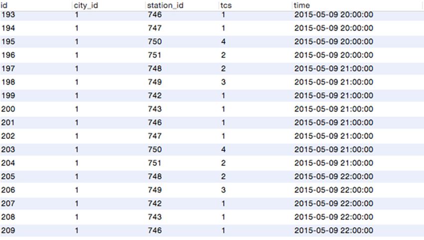
3.1.3. Point of Interest
A point of interest, or POI, is a specific location that someone may be interested in. For example,
restaurants and
Sensors 2016, 16, shopping
86 malls surrounding us are POI. Figure 4 presents the restaurant6locations
of 18
Sensors 2016, 16, 86
around Sanhao Street of Shenyang on Google Maps. 6 of 18
Figure 4.4.POI
Figure POInear
POI nearthe
near theSanhao
the Sanhao streetofofShenyang
Sanhao street
street Shenyang city.
city.
3.2.
3.2. Problem
Problem Formulation
Formulation
This
This paper
paper uses
uses urbanurban sensing
sensing data
data toto solve
solve the
the problem
problem of of air
air quality
quality inference
inference which
which means
means toto
infer the unknown air quality of areas by using all kinds of data. These
infer the unknown air quality of areas by using all kinds of data. These data affect either the sourcesdata affect either the sources
of
of air
air pollution
pollution such
such as as traffic emissions and
traffic emissions and point
point of of interest distribution or
interest distribution their results
or their results suchsuch as the
as the
air
air quality
quality index,
index, so so establishing
establishing thethe relationship between these
relationship between these data
data and
and air
air quality
quality is is the
the key
key to
to this
this
kind of approach. The RAQ algorithm collects several kinds of related
kind of approach. The RAQ algorithm collects several kinds of related data including air monitoring data including air monitoring
station data (AQI),
station data (AQI),meteorology
meteorologydata data (MD),
(MD), traffic
traffic (TCS),
(TCS), road road information
information (RI) POI
(RI) and and data.
POI data. All
All these
these
data aredata are fetched
fetched at intervalsat intervals of one
of one hour. Wehour.
divide We thedivide thegrids
city into city (G)
intoand
grids (G)grid
each andis each grid as
regarded is
regarded as one unit. Those grids (G ) with air quality monitoring stations
one unit. Those grids (G1 ) with air quality monitoring stations generate the data with the label AQI
1 generate the data with the
label AQI
while while(Gthe
the grids grids (G2) without stations generate the data used for prediction. Data from G1
2 ) without stations generate the data used for prediction. Data from G1 are used for
are
training our learning our
used for training modellearning model
and data fromandG2data
are from
inputGinto 2 are theinput
modelintotothe model the
generate to generate
predicationthe
predication value. The only difference of data from G and G is data
value. The only difference of data from G1 and G2 is data from G1 are labeled as an AQI value. The
1 2 from G 1 are labeled as an AQI
value.
results The results
are given asare given AQI
different as different
levels. IfAQI levels.value
the actual If thefrom
actual value from
monitoring monitoring
stations belongsstations
to this
belongs to this AQI level, then we know the prediction is
AQI level, then we know the prediction is right. Otherwise the prediction is wrong.right. Otherwise the prediction is wrong.
This problem can
This problem canbe beformulated
formulatedas asfollows:
follows:given
givena acollection
collectionofofgridsgridsGG = =G1GY
1 ∪G G22 (|G ≪|G
(|G11||! |G22|),
|),
where gg11¨·AQI
where AQI (g(g11 P GG11)) is known and
is known and gg22¨·AQI
AQI (g(g22 PG G22)) is unknown, g¨
is unknown, g·MD,
MD, g¨g·TCS,
TCS, g¨g·RI
RI and
and g¨g·POI
POI are
are
known
known (g G),
(g P G), RAQ
RAQ aims aims to to predict
predictgg22¨·AQI
AQI atat intervals
intervals of of one
one hour.
hour.
4. RAQ
RAQAlgorithm
Algorithm
In the RAQ algorithm, all data are collected from the urban sensing system including air
monitoring station
stationdata,
data,meteorology
meteorology data,
data, traffic
traffic data, data, road information
road information and POIand dataPOIand data and
necessary
necessary
features are features are extracted
extracted from heterogeneous
from heterogeneous data. Thesedata. These features
features are the
are the most most common
common data indata
city
in city life. Traffic-related sources like vehicle emissions and POI like factories are
life. Traffic-related sources like vehicle emissions and POI like factories are the main sources for air the main sources
for air pollutants
pollutants [3]. Meteorology
[3]. Meteorology is the
is the main main approach
approach for dispersion
for dispersion of air pollutants
of air pollutants [3]. These[3]. These
data can
data can well
represent represent
the airwell the situation.
quality air quality situation.
The training The training
dataset dataset
includes includes
all the necessary all features
the necessary
and is
features and subsets
divided into is divided
usinginto subsets technology.
bootstrap using bootstrap technology.
Figure 5 shows theFigure 5 shows
structure of thethe structure
dataset. of the
A decision
dataset. A decisionon
tree is constructed tree is constructed
each subset, and theon each subset, and
classification the classification
is done by aggregating is done by aggregating
the results generated
the
from results generated
all decision trees.from all decision
Figure 6 shows trees. Figure 6 of
the procedure shows
the RAQthe procedure
algorithm.of the RAQ algorithm.
Figure 5.
Figure Dataset structure.
5. Dataset structure.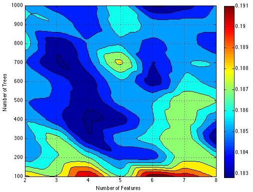
Sensors 2016, 16, 86 7 of 18
Sensors 2016, 16, 86 7 of 18
Figure 6.
Figure The procedure
6. The procedure of
of RAQ.
RAQ.
4.1. Data Collection and Feature Extraction
4.1.1. Meteorology Data
4.1.1. Meteorology Data
Meteorology data
Meteorology data such
such asas temperature
temperature and and humidity
humidity areare very
very important factors that
important factors that severely
severely
affect the concentration and spread of air pollutants. Understanding the behavior
affect the concentration and spread of air pollutants. Understanding the behavior of meteorological of meteorological
parameters
parameters in in the
the planetary
planetary boundary layer is
boundary layer is important
important because the atmosphere
because the atmosphere is is the
the medium
medium in in
which air pollutants are transported away from the source, which is governed by
which air pollutants are transported away from the source, which is governed by the meteorologicalthe meteorological
parameters such as
parameters such as atmospheric
atmospheric windwind speed,
speed, wind
wind direction,
direction, and
and temperature
temperature [32]. [32]. In
In this
this paper,
paper, we
we
use
use weather
weather monitoring
monitoring stations
stations as
as one
one part
part of
of the
the urban
urban sensing
sensing system. Considering the
system. Considering the accessibility
accessibility
of
of the
the data,
data, we
we use
usefollowing
followingmeteorology
meteorology datadatafeatures:
features: temperature
temperature (F (Fmt , ˝ C), humidity (F mh,, %),
mt, °C), humidity (Fmh
%),
barometric pressure (F
barometric pressure (Fmp mp , mmHg), wind speed
, mmHg), wind speed (Fmwmw (F , m/s) and visibility (F
, m/s) and visibility (Fmv, m).
mv , m).
4.1.2. Traffic and
4.1.2. Traffic and Road
Road Data
Data
Traffic is
Traffic is one
one of
of the
the most
most important
important factors
factors that
that affect
affect the
the air quality. Figure
air quality. Figure 33 is is aa sample
sample of of the
the
original data that is available from map service providers. In this paper, we
original data that is available from map service providers. In this paper, we rely on two important rely on two important
characteristics
characteristics of of traffic,
traffic, which
which areare road
road length
length (F(Frlrl)) and
and traffic
traffic congestion
congestion status
status (F(Ftcs ). If the road is
tcs). If the road is
very
very long and traffic congestion is relatively light, exhaust gas emissions can be at level
long and traffic congestion is relatively light, exhaust gas emissions can be at a high a highbecause
level
of the total number of vehicles on this road. Similarly, if a road is short and
because of the total number of vehicles on this road. Similarly, if a road is short and traffic traffic congestion is heavy.
However,
congestionwe do not have
is heavy. a method
However, we do or not
accurate
have data
a method to quantify these data
or accurate two characteristics
to quantify these directly.
two
Most map service providers offer online maps and real-time traffic status. They
characteristics directly. Most map service providers offer online maps and real-time traffic status. do not publish public
application
They do notinterfaces (APIs) application
publish public for third party developers
interfaces (APIs)to access
for thirdthese data,
party but we can
developers tostill get some
access these
useful hints through analyzing the web http requests of the map. Essentially,
data, but we can still get some useful hints through analyzing the web http requests of the these data are collected
map.
from GPS equipment installed in cars or speed measurement sensors.
Essentially, these data are collected from GPS equipment installed in cars or speed measurement These data denote another
important part of
sensors. These thedenote
data urban sensing
another systems.
important Figure
part of 7 shows
the urbanthe http request
sensing records
systems. of a typical
Figure 7 showsBaidu
the
map when we invoke the traffic widget.
http request records of a typical Baidu map when we invoke the traffic widget.
As we know, a picture is composed of many pixels, so a picture can be digitized into a matrix. We
use the colored pixel distribution to represent the information of road length and congestion status.
For each tile grid, we count the quantity of pixels to represent the road. The larger the quantity of
pixels, the greater the length of the road is in one tile grid.
As shown in Figure 3, traffic congestion status is denoted by different colors (green, orange and
red) in the pixels which represent roads. According to the traffic volume of different congestion levels,
different weights are assigned to the numbers of pixels in different colors (1, 2 and 5). In Figure 8, the
weighted tcs value is calculated by formula a + 2b + 5c, where a is the number of pixels in green, b is
the number of pixels in orange and c is the number of pixels in red.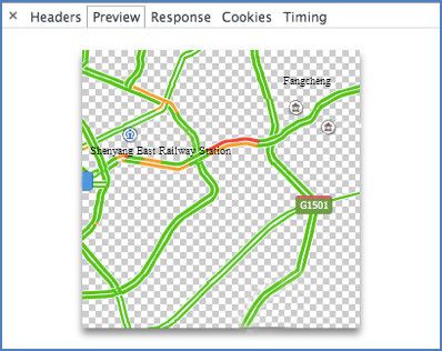
Sensors 2016, 16, 86                                                                                        8 of 18
Sensors 2016, 16, 86                                                                                                   8 of 18

                               Figure 7. HTTP request analysis by Chrome developer tool.

           As we know, a picture is composed of many pixels, so a picture can be digitized into a matrix. We
      use the colored pixel distribution to represent the information of road length and congestion status.
      For each tile grid, we count the quantity of pixels to represent the road. The larger the quantity of
      pixels, the greater the length of the road is in one tile grid.
           As shown in Figure 3, traffic congestion status is denoted by different colors (green, orange and
      red) in the pixels which represent roads. According to the traffic volume of different congestion
      levels, different weights are assigned to the numbers of pixels in different colors (1, 2 and 5). In
      Figure 8, the weighted tcs value is calculated by formula a + 2b + 5c, where a is the number of pixels
      in green, b is the number
                            Figureof 7.
                                     pixels
                                Figure  HTTP
                                        7.   in request
                                           HTTP orange  and  c is the
                                                 requestanalysis
                                                         analysis     numberdeveloper
                                                                   by Chrome
                                                                  by  Chrome of pixelstool.
                                                                             developer intool.
                                                                                          red.

     As we know, a picture is composed of many pixels, so a picture can be digitized into a matrix. We
use the colored pixel distribution to represent the information of road length and congestion status.
For each tile grid, we count the quantity of pixels to represent the road. The larger the quantity of
pixels, the greater the length of the road is in one tile grid.
     As shown in Figure 3, traffic congestion status is denoted by different colors (green, orange and
red) in the pixels which represent roads. According to the traffic volume of different congestion
levels, different weights are assigned to the numbers of pixels in different colors (1, 2 and 5). In
Figure 8, the weighted tcs value is calculated by formula a + 2b + 5c, where a is the number of pixels
in green, b is the number of pixels in orange and c is the number of pixels in red.

                                            Figure 8.
                                            Figure    Traffic congestion
                                                   8. Traffic congestion status.
                                                                         status.

      4.1.3. POI Data
          The category of POIs and their density in a region indicate the land use and the function of the
     region as
             as well
                well as
                      as the
                          thetraffic
                              trafficpatterns
                                      patternsininthe
                                                   theregion,
                                                        region,therefore
                                                                 thereforecontributing toto
                                                                            contributing  thethe
                                                                                               airair
                                                                                                   quality inference
                                                                                                      quality         of
                                                                                                              inference
     the region
     of the     [24].
            region    ForFor
                   [24].    example,  shopping
                               example,   shoppingstreets are more
                                                      streets       likely
                                                              are more     to gather
                                                                         likely      moremore
                                                                                to gather  people   than parks
                                                                                                 people         so there
                                                                                                         than parks   so
     will be more human-related air pollution sources like vehicles. Schools always have more green areas
     than factories so there are more plants to absorb the air pollutants. Therefore, POI distribution has a
     strong effect on air quality. These data also imply the significance of human activities in urban sensing
     systems. In this paper, the number of POI is counted in each tile grid. According to the searching
     results of Baidu maps and Google Map, the majority of POI are divided into ten categories. Table 2
     shows the categories and Figure 9 presents the number of POI (F pn ) in each category.
                                          Figure 8. Traffic congestion status.

4.1.3. POI Data
      The category of POIs and their density in a region indicate the land use and the function of the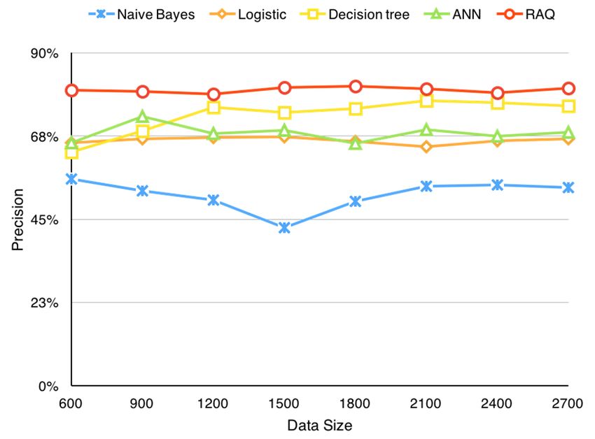
ten categories. Table 2 shows the categories and Figure 9 presents the number of POI (Fpn) in each
category.
Table 2. POI categories.
Sensors 2016, 16, 86 9 of 18
Code POI Category
P1 Transportation
Table 2. POI categories.
P2 Entertainment
CodeP3 Restaurant
POI Category
P1 P4 Education
Transportation
P2 P5 Entertainment
Residential District
P3 Restaurant
P4 P6 Park
Education
P5 P7 Residential
Company District
P6 Park
P8 Factory
P7 Company
P8 P9 Shopping mall
Factory
P9P10 Gas station mall
Shopping
P10 Gas station
Number
7000 6307
5418
5078
5250
3853
Number
3354
3500 2541
1750 879 1050
147 178
0
p1 p2 p3 p4 p5 p6 p7 p8 p9 p10
POI Categories
Figure 9. Numbers of POI in Shenyang city.
Figure 9. Numbers of POI in Shenyang City.
4.2. Random
4.2. Random Forest
Forest Classification
Classification
The Random
The Random ForestForest is is aa general
general termterm forfor ensemble
ensemble methods using tree-type
methods using tree-type classifiers
classifiers
h( x, θkk),q,kk“1,...,}
{thpx, 1, ..., where
u where thethe{tθ
k}
areindependent
k uare independentidentically
identically distributed
distributed random
random vectors
vectors and
and x isx
is an input pattern, hpx, is a generated classifier [33]. It uses recursive partitioning
an input pattern, h( x, kk ) is a generated classifier [33]. It uses recursive partitioning to generate
θ q to generate many
trees and
many trees then
andaggregate the results.
then aggregate Each tree
the results. is independently
Each constructed
tree is independently using a using
constructed bootstrap sample
a bootstrap
of the training
sample data, which
of the training data,subdivides
which subdividesthe parameter set firstset
the parameter into several
first parts depending
into several on oneon
parts depending of
the parameters, and subsequently repeats the process
one of the parameters, and subsequently repeats the process for each part. for each part.
4.2.1. Bootstrap
4.2.1. Bootstrap Aggregating
Aggregating (Bagging)
(Bagging)
There is
There is usually
usually aa single
single data
data sample
sample inin each
each class
class for
for training.
training. A A simple
simple method
method isis to
to divide
divide the
the
dataset into non-overlapping subsets and construct the trees independently. However,
dataset into non-overlapping subsets and construct the trees independently. However, this requires this requires
aa huge
huge amount
amount of of data
data and
and itit cannot
cannot always
always bebe guaranteed
guaranteed in in different
different situations.
situations. AA better
better way
way is
is
sampling the original dataset with replacement for a certain times to produce a
sampling the original dataset with replacement for a certain times to produce a bootstrap sample. bootstrap sample.
This method
This method ensures
ensures that
that the
the samples’
samples’ distributions
distributions are
are statistically
statistically identical
identical with
with the
the original
original data
data
sample [34].
sample [34]. There are nn records
There are records in
in the
the original
original dataset
dataset and
and soso the
the probability
probability of
of each
each record
record is
is
constantly 1/n. The probability of not selecting a certain record is (1 – 1/n), which results in (1 – 1/n)n
when repeated n times.
Assuming the sample size tends to be infinite, the probability can be expressed as
limn Ñ8 (1 – 1/n)n which is equal to e´1 . Therefore, the probability of selecting one record is
(1 – e´1 ) « 2 /3 . Thus, in each bootstrap sample there are about 2 /3 original samples for training.
4.2.2. Tree Growing and Splitting
As we know, a decision tree starts with one root node. In the following process, the samples
are split into different spaces using one of the features including monitoring station data (AQI),
meteorology data(MD), traffic(TCS), road information(RI) and POI data.. Therefore, how to select the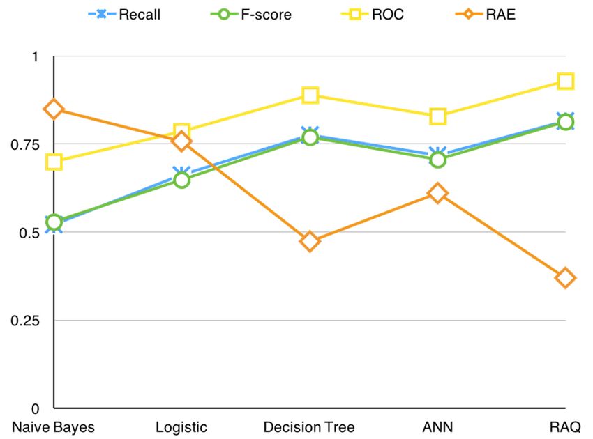
Sensors 2016, 16, 86                                                                                    10 of 18

feature in each split is of great significance for the performance of a decision tree. Information gain [35]
is usually used as the criterion for classifiers.
     The features selection for each bootstrap sample is randomized. According to bagging theory,
random forest is strong classifier based on multiple weak classifiers. Therefore, both the number of
data and the number of features of the subset are smaller than original dataset’s. We need T subsets
with m features. According to Brieman’s suggestions [33], m is much less than the number of all the
                                                             1? ?        ?
features. Brieman suggests three possible values for m:        m, m, 2 m. In the evaluation section, we
                                                             2
would show four features and 400 subsets are best for our model and dataset.
     When splitting the dataset, for each feature candidate, entropy is calculated as in Equation (3):

                                                          k
                                                          ÿ
                                      Entropypcq “ ´             ppci qlog2 ppci q                           (3)
                                                          i “1

                                                             Ni
                                                ppci q “                                                     (4)
                                                            k
                                                            ř
                                                              Ni
                                                            i “1

where ci is the AQI level i which is specified in Table 1, the probability p(ci ) is calculated through
Equation (2) where Ni is the quantity of records in different AQI level and k is the number of AQI
levels. Therefore, the information gain is defined as shown in Equation (5):
                                                                   ˇ ˇ
                                                                   ˇ jˇ
                                                                 w ˇf ˇ
                                                                 ÿ   i
                               Gainp f i q “ Entropypcq ´                       Entropyp f j i q             (5)
                                                                       | fi |
                                                                 j“1

where fi represents records of the ith level of tree, fi j are records in jth node of the ith level of tree, and
w is the number of nodes in this level.
      The process of splitting stops when: (a) the records in one node fall below the threshold value
defined by users; (b) the node is pure which means all the records fall into one class. For the terminated
node has unordered records, the percentage of different classes are calculated and so the predicted
class is defined as in Equation (6):

                                             Cpiq “ Maxpppci qq                                              (6)

4.3. Prediction
       After all the trees are constructed, the unlabeled data are input into all decision trees. For each tree,
p(ci ) is the estimated probability of the AQI level i. The final probability of the AQI level i p’(ci ) in the
random forest is defined in Equation (7), where T is the number of decision trees as mentioned before:

                                                            T
                                                          1ÿ
                                             p1 pci q “       ppci q                                         (7)
                                                          T
                                                            k“1

      The final result is determined by Equation (8):

                                             C1 piq “ Maxpp1 pci qq                                          (8)

      The pseudocode of RAQ algorithm is described in Algorithm 1.
Sensors 2016, 16, 86 11 of 18
Algorithm 1. RAQ
A dataset S with features: Fmt , Fmh , Fmp , Fmw , Fmv , Fri , Ftcs , F pn and labeled AQI level;
Input:
unlabeled dataset U; trees quantity T; features quantity m;
Output: AQI level
1 for T trees
2 randomly select m features from S;
3 for m features in each node
4 calculate information gain by Equation (3);
5 choose maximum gain to split the dataset in the node;
6 remove used feature from feature candidates;
7 input unlabeled data into trees;
5 get predicted AQI level according to Equations (5) and (6);
5. Evaluation
5.1. Dataset
In the experiments, one-month data from 4 May 2015 to 5 June 2015 is collected and the following
four datasets of Shenyang are used which are all available to the public. In our testing period, we
use a total of 2701 data to test this algorithm and Shenyang is divided into 1258 grids corresponding
to 34 rows and 37 columns. Because all the grids belong to the main city area, all data including
meteorology data, traffic data, road information and POI data in these grids are accessible from our
data sources. Air quality data is accessible in the areas covered by air monitoring stations.
5.1.1. Monitoring Station Data
The air quality information from the Shenyang monitoring stations includes AQI, the
concentrations of CO, NO2 , SO2 , O3 , PM10 and PM25 and timestamp. Table 3 shows the format
of the monitoring station data. Table 4 shows the locations of all the monitoring stations. All the
data are collected from the public website [36] whose data are produced by National Department of
Environmental Protection. We use the Java programming language to access the API interface hourly
and store all the data into a MySQL database.
Table 3. Data samples of monitoring stations.
CO NO2 SO2 O3 PM10 PM25
Station_id Aqi Time
(µg/m3 ) (µg/m3 ) (µg/m3 ) (µg/m3 ) (µg/m3 ) (µg/m3 )
747 77 1.802 70 69 63 104 52 2015-05-24 03:00
750 139 2.233 62 70 57 125 106 2015-05-24 03:00
751 82 1.706 73 58 69 100 60 2015-05-24 03:00
741 85 1.942 80 64 43 94 63 2015-05-24 03:00
748 63 1.024 61 62 68 76 37 2015-05-24 04:00
749 67 1.358 60 29 62 81 48 2015-05-24 04:00
742 88 1.646 97 82 12 125 14 2015-05-24 04:00
743 84 0.808 68 167 45 117 52 2015-05-24 04:00
744 98 1.718 66 56 43 92 73 2015-05-24 04:00
745 86 1.333 78 72 9 121 37 2015-05-24 04:00
746 66 1.229 66 24 48 82 45 2015-05-24 04:00
747 63 1.175 58 48 70 75 36 2015-05-24 04:00Sensors 2016, 16, 86 12 of 18
Table 4. Locations of monitoring stations.
Station_id Latitude Longitude
741 41.841445 123.65436
742 41.758166 123.533761
743 41.71694 123.451378
744 41.788094 123.288852
745 41.838551 123.549754
746 41.855605 123.442396
747 41.773208 123.421573
748 41.785295 123.489395
749 41.79609169 123.4084114
750 41.789429 123.373275
751 41.83933982 123.4126515
5.1.2. Meteorological Data
We collect meteorological data including temperature, humidity, barometric pressure, wind speed
and visibility from the public website [37]. As Table 5 illustrates, the data format is presented as
temperature (Fmt ), humidity (Fmh ), barometric pressure (Fmp ), wind speed (Fmw ) and visibility (Fmv ).
Table 5. Meteorological samples.
Temperature Barometric Pressure Humidity Wind Speed Visibility
Time
(Fmt , ˝ C) (Fmp , mmHg) (Fmh , %) (Fmw , m/s) (Fmv , m)
18.8 748.6 56 2 16.0 2015-05-14 11:00:00
18.3 746.4 50 7 26.0 2015-05-14 08:00:00
17.0 744.6 63 3 12.0 2015-05-14 05:00:00
18.4 743.0 58 1 16.0 2015-05-14 02:00:00
19.7 743.9 63 1 18.0 2015-05-13 23:00:00
18.0 742.6 72 0 7.0 2015-05-13 21:00:00
5.1.3. Road and Traffic Data
There are no public websites that offer statistical road and traffic data. Therefore, we cannot
directly get available formatted data. However, most of the map service providers offer online maps
and real-time traffic status. They do not publish public API interfaces for third party developers to
access these data, but we can still get some useful tips through analyzing the map web http requests.
From map services providers [38,39], we collect the traffic map tiles every hour.
5.1.4. POI
Thank to Baidu map and Google map service, we can easily get these data from a public interface.
Each POI record contains name, latitude, longitude, tag and located tile grids. Figure 10 shows about
28,000 records in the MySQL database.Sensors 2016, 16, 86 13 of 18
Sensors 2016, 16, 86 13 of 18
Figure 10.10.
Figure POIPOISamples
Samples inin Shenyang.
Shenyang.
5.2. Evaluation Method
5.2. Evaluation Method
The most accurate criterion for air quality measure is the air quality information from monitoring
The most accurate
stations. criterionwe for
In this experiment, airAQI
use the quality
data frommeasure
monitoringis the asairthequality
stations information from
reference standard.
monitoringTostations.
construct aIn random
this forest, we need towe
experiment, determine
use the two parameters
AQI datawhich from are monitoring
the numbers of trees
stations as the
and the number of features used to construct each tree. To choose the best parameters, we use OOB
reference standard. To construct a random forest, we need to determine two parameters which are
(Out-of-Bag) [33] error to compare RAQ accuracy based on different parameters pairs which andmeansthe number
the number of features
of features used to used to each
construct construct each
tree and the tree.ofTo
number treeschoose
that the best
parameters,arewe use OOB
constructed in the(Out-of-Bag)
random forest. In [33] error
random to compare
forests, RAQ accuracy
the error is estimated basedtheon different
internally during
parameters construction of trees. Each tree is constructed using a different bootstrap sample from original data,
pairs which means the number of features used to construct each tree
which about one-third are left out of the bootstrap sample. The one-third sample is used as test cases
and the number of trees
to be input into thethat aregetconstructed
tree and the classificationinoftheeachrandom forest.
test case. At the endIn of random
the run, takeforests,
the class the error is
estimated internally
j that got most during
of the votestheevery
construction
time case n was of oob
trees. Each
[40]. The tree isofconstructed
proportion using
times that j is not equal a different
to the true class of n averaged over all cases is the oob error estimate
bootstrap sample from original data, which about one-third are left out of the bootstrap [40]. The smaller number of oob,sample. The
the high accuracy of the model. For the number of features, we increase by one each time from 2 to
one-third sample is used as test cases to be input into the tree and get the classification of each test
8 (total number of features is 8 specified in algorithm ). For the quantity of trees, we increase by 100
case. At thefrom
end100of tothe run,
1000. take ofthe
Because theclass j that got most
time consumption of the
with more votes
number of every
trees, wetime
ignorecase n was oob [40].
the trees
The proportion
number of greater
times than that1000
j is and
not 100
equal
gap istosuitable
the true class of
to balance n averaged
performance and over all To
accuracy. cases is the oob error
compare
this algorithm with others, we use cross-validation method to judge the performance.
estimate [40]. The smaller number of oob, the high accuracy of the model. For the number of
features, we5.3.increase
Results by one each time from 2 to 8 (total number of features is 8 specified in
algorithm ).5.3.1.
ForEffects
the of quantity of trees, we increase by 100 from 100 to 1000. Because of the time
Parameters on Prediction Error Rate
consumption with more number of trees, we ignore the trees number greater than 1000 and 100 gap
There are two important factors that affect the performance of a random forest, which are the
is suitable to balance
number of trees performance
and features. Figureand11accuracy.
shows how the ToOOBcompare this algorithm
error changes along with thewith
number others,
of we use
cross-validation
featuresmethod
and trees.to judge
X-axis the
is the performance.
number of features and Y-axis is the number of trees.
5.3. Results
5.3.1. Effects of Parameters on Prediction Error Rate
There are two important factors that affect the performance of a random forest, which are the
number of trees and features. Figure 11 shows how the OOB error changes along with the number of
features and trees. X-axis is the number of features and Y-axis is the number of trees.Sensors 2016, 16, 86 14 of 18
Sensors 2016, 16, 86 14 of 18
Figure 11. OOB
Figure 11. OOB error
error result
result distribution.
distribution.
Empirically, for
Empirically, for our
our experiment,
experiment, we
we choose
choose integer
integer as the
the number
number of features
features and
and 100
100 interval
interval
number of trees,
integer as the number trees, so
so only
only the
the discrete
discrete coordinate
coordinate values
values such
such as
as (2,100),
(2,100), (3,200) are
meaningful in this graph.
graph. Different
Differentcolors
colorsmean
meandifferent
differentOOB
OOBerror
errorvalues.
values.The
Thedeeper
deeper thethe
color is,
color
the smaller the oob is. As the graph shows, the OOB errors reach the best when the parameters
is, the smaller the oob is. As the graph shows, the OOB errors reach the best when the parameters pairs
are and and
. lessless
Considering time
timeconsumption,
consumption,we wechoose
choose
as as the
the best
parameters pair.
parameters pair.
5.3.2. Comparison
For the contrast tests, Naïve Bayes, Logistic Regression, Single Decision Tree and ANN
For the contrast tests, Naïve Bayes, Logistic Regression, Single Decision Tree and ANN are
are chosen. Here we use Weka [41] as the tool to conduct all the comparison tests. For
chosen. Here we use Weka [41] as the tool to conduct all the comparison tests. For Naïve Bayes, there
Naïve Bayes, there are eight features which are Fmt , Fmh , Fmp , Fmw , Fmv , Fri , Ftcs , Fpn and six
are eight features which are Fmt, Fmh, Fmp, Fmw, Fmv, Fri,,Ftcs, Fpn and six classification categories (C)
classification categories (C) which are specified in Table 1. In Weka, this algorithm is denoted as
which are specified in Table 1. In Weka, this algorithm is denoted as
weka.classifiers.bayes.NaiveBayesMultinomial.
weka.classifiers.bayes.NaiveBayesMultinomial. For For Logistic
Logistic Regression,
Regression, we choose
we choose Multinomial
Multinomial Logistic
Logistic Regression because of the multi AQI levels. In
Regression because of the multi AQI levels. In Weka, this algorithm is denoted Weka, this algorithm is denoted as as
weka.classifiers.functions.Logistic.
weka.classifiers.functions.Logistic. For For Single
Single Decision
Decision Tree,
Tree, wewe choose
choose all all
thethe features
features to construct
to construct one
one
singlesingle
tree tree for classification.
for classification. In Weka,
In Weka, this this algorithm
algorithm is denoted
is denoted as weka.classifiers.trees.REPTree.
as weka.classifiers.trees.REPTree. For
For ANN, we choose back-propagation neural network
ANN, we choose back-propagation neural network with one hidden layer with one hidden layerfor
for its
its simplicity
simplicity and
and
generality.
generality. In In Weka,
Weka, this
thisalgorithm
algorithmisisdenoted
denotedasasweka.classifiers.functions.MultilayerPerceptron.
weka.classifiers.functions.MultilayerPerceptron.
After
After realizing
realizingdifferent
differentalgorithms,
algorithms, tests areare
tests carried out.out.
carried Table 6 shows
Table the results
6 shows of theoftest
the results thecases
test
in
cases in which Y means correct predictions and N means incorrect predictions. The precisionby
which Y means correct predictions and N means incorrect predictions. The precision is calculated is
the formulaby
calculated Y/(Y
the+formula
N) where Y is+the
Y/(Y N)number
where Y of is
correct predictions
the number and N is
of correct the number
predictions of incorrect
and N is the
predictions. Figure 12predictions.
number of incorrect illustrates how the 12
Figure prediction
illustratesprecision
how the changes as theprecision
prediction data sizechanges
changes.asThisthe
figure shows RAQ performs steadily, even when the data size is relatively small.
data size changes. This figure shows RAQ performs steadily, even when the data size is relatively Other algorithms are
less
small.accurate
Other at all time. are less accurate at all time.
algorithms
Table 6. Precision table of different algorithms.
Table 6. Precision table of different algorithms.
AlgorithmAlgorithm Precision
Precision Y Y N N
NaïveBayes 52.1% 1408 1293
NaïveBayes 52.1% 1408 1293
Logistic Logistic 66.2%
66.2% 17901790911 911
Decision Decision
Tree Tree 77.4%
77.4% 20922092609 609
ANN ANN 71.8%
71.8% 19401940761 761
RAQ RAQ 81.5%
81.5% 22032203498 498Sensors 2016, 16, 86 15 of 18
Sensors 2016, 16,
Sensors 2016, 16, 86
86 15
15of
of18
18
Figure 12. Precision changes according to data size.
Besides the precision FigureFigure 12. Precision
12.
measurement, wechanges
Precision according
also refer
changes to
to data
to other
according size.
measurements
data size. including Recall,
F-score, Relative Absolute Error (RAE) and Receiver Operating Characteristic (ROC). Recall is the
Besidesofthe
Besides
proportion the precision
precision
instances measurement,
measurement,
classified we we
as a given also also
classreferrefer to the
to other
divided by other measurements
measurements
actual in that including
total including Recall,
class. Recall,
F-score,
F-score is a
F-score,
Relative Relative
Absolute Absolute
Error Error
(RAE) and (RAE) and
Receiver Receiver
Operating Operating
CharacteristicCharacteristic
(ROC). (ROC).
Recall
combined measure for precision and recall calculated as 2 Precision Recall/(Precision + Recall) where is theRecall is the
proportion
proportion
of (alsoof
instances
Recall instances
classified
known classified
asassensitivity) asisa the
a given class given
dividedclass
by divided
fraction the
of actual bytotal
relevant the actual
in thattotal
instances thatinare
class. that
F-scoreclass.
is aF-score
retrieved. combinedis a
Relative
combinederror
measure
absolute measure
for for precision
precision and by
is calculated theand
recall recall calculated
calculated
following formula: as 2 Precision Recall/(Precision
as 2˚Precision˚Recall/(Precision + Recall)+ where
Recall) Recall
where
Recallknown
(also (also known as sensitivity)
as sensitivity) is the fraction
is the fraction of Nrelevant
of relevant instancesinstances that are retrieved.
that are retrieved. Relative
Relative absolute
absolute
error error is calculated
is calculated by the following
by the following formula:RAE
formula:
i 1 i
ri
ř NNi 1 rri
N
RAE
|θi 1 ´i r |i
RAE “ i“1 ˇ´i iˇ
i“
ř N ˇˇN
where i is the estimated value, ri is the real value, 1 ̅ ´
rˇi average value, N is the number of test
isrithe
ˇ
1 ˇiθ ˇ
cases. ROC shows how the number of correctly classified positive examples varies with the number
where
where
of θi iis is
incorrectly the
the estimated
estimated
classified value,
negative ri ris
value,examples
i is
thethereal
[42]. value,θ is̅ is
realvalue, thethe averagevalue,
average value,NNisisthe
thenumber
number of
of test
test
cases. ROC
cases. ROC showsshows howhowthe
thenumber
numberofofcorrectly
correctlyclassified
classifiedpositive positive examples
examples varies
varies with
with thethe number
number of
of incorrectly
incorrectly classified
classified negative
negative examples
Table
examples 7. [42].
Indexes
[42]. of different algorithms.
Algorithm Recall F-Score ROC RAE
Table 7.
Table 7. Indexes of
of different
different algorithms.
algorithms.
Naive Bayes 0.521 0.529 0.7 84.9%
Algorithm Recall F-Score ROC RAE
AlgorithmLogistic Recall0.663 F-Score
0.649 0.785
ROC 75.8% RAE
Naive Bayes
Decision Tree 0.521 0.529 0.7 84.9%
Naive Bayes 0.521 0.775 0.5290.769 0.888
0.7 47.4% 84.9%
Logistic 0.663
Logistic ANN 0.663 0.718 0.649 0.649
0.707 0.785 75.8%
0.785 60.9%
0.829 75.8%
DecisionDecision
Tree
RAQ 0.775
Tree 0.775
0.816 0.769
0.769
0.814 0.888 36.9%
0.888
0.928 47.4% 47.4%
ANN 0.718 0.707 0.829 60.9%
ANN 0.718 0.707 0.829 60.9%
RAQ 0.816 0.814 0.928 36.9%
RAQ 0.816 0.814 0.928 36.9%
Figure 13. Indexes chart of different algorithms.
Figure 13. Indexes chart of different algorithms.You can also read