Decreasing uncertainty in flood frequency analyses by including historic flood events in an efficient bootstrap approach
←
→
Page content transcription
If your browser does not render page correctly, please read the page content below
Nat. Hazards Earth Syst. Sci., 19, 1895–1908, 2019
https://doi.org/10.5194/nhess-19-1895-2019
© Author(s) 2019. This work is distributed under
the Creative Commons Attribution 4.0 License.

Decreasing uncertainty in flood frequency analyses by including
historic flood events in an efficient bootstrap approach
Anouk Bomers1 , Ralph M. J. Schielen1,2 , and Suzanne J. M. H. Hulscher1
1 Department     of Water Engineering and Management, University of Twente, Dienstweg 1, Enschede, the Netherlands
2 Ministry   of Infrastructure and Water Management (Rijkswaterstaat), Arnhem, the Netherlands

Correspondence: Anouk Bomers (a.bomers@utwente.nl)

Received: 15 March 2019 – Discussion started: 18 March 2019
Revised: 18 July 2019 – Accepted: 9 August 2019 – Published: 29 August 2019

Abstract. Flood frequency curves are usually highly uncer-           Return periods of design discharges are commonly of the
tain since they are based on short data sets of measured dis-     order of 500 years or even more, while discharge measure-
charges or weather conditions. To decrease the confidence         ments have been performed only for the last 50–100 years.
intervals, an efficient bootstrap method is developed in this     For the Dutch Rhine river delta (used as a case study in this
study. The Rhine river delta is considered as a case study. We    paper), water levels and related discharges have been regis-
use a hydraulic model to normalize historic flood events for      tered since 1901 while design discharges have a return period
anthropogenic and natural changes in the river system. As a       up to 100 000 years (Van der Most et al., 2014). Extrapolation
result, the data set of measured discharges could be extended     of these measured discharges to such return periods results in
by approximately 600 years. The study shows that historic         large confidence intervals of the predicted design discharges.
flood events decrease the confidence interval of the flood fre-   Uncertainty in the design discharges used for flood risk as-
quency curve significantly, specifically in the range of large    sessment can have major implications for national flood pro-
floods. This even applies if the maximum discharges of these      tection programmes since it determines whether and where
historic flood events are highly uncertain themselves.            dike reinforcements are required. A too wide uncertainty
                                                                  range may lead to unnecessary investments.
                                                                     To obtain an estimation of a flood with a return period of
                                                                  10 000 years with little uncertainty, a discharge data set of at
1   Introduction
                                                                  least 100 000 years is required (Klemeš, 1986). Of course,
Floods are one of the main natural hazards to cause large eco-    such data sets do not exist. For this reason, many studies
nomic damage and human casualties worldwide as a result           try to extend the data set of measured discharges with his-
of serious inundations with disastrous effects. Design dis-       toric and/or paleo-flood events. The most common methods
charges associated with a specific return period are used to      in literature to include historical data in an FFA are based
construct flood defences to protect the hinterland from severe    on the traditional methods of frequentist statistics (Frances
floods. These design discharges are commonly determined           et al., 1994; MacDonald et al., 2014; Sartor et al., 2010) and
with the use of a flood frequency analysis (FFA). The ba-         Bayesian statistics (O’Connell et al., 2002; Parkes and De-
sic principle of an FFA starts with selecting the annual max-     meritt, 2016; Reis and Stedinger, 2005).
imum discharges of the measured data set, or peak values             While frequentist statistics are generally applied by deci-
that exceed a certain threshold (Schendel and Thongwichian,       sion makers, Bayesian statistics have significantly increased
2017). These maximum or peak values are used to identify          in popularity in the last decade. Reis and Stedinger (2005)
the parameters of a probability distribution. From this fitted    have successfully applied a Bayesian Markov chain Monte
distribution, discharges corresponding to any return period       Carlo (MCMC) analysis to determine flood frequency rela-
can be derived.                                                   tions and their uncertainties using both systematic data and
                                                                  historic flood events. A Bayesian analysis determines the full

Published by Copernicus Publications on behalf of the European Geosciences Union.
1896 A. Bomers et al.: Decreasing uncertainty in flood frequency analyses posterior distribution of the parameters of a probability dis- events based on the current geometry. In such a way, the tribution function (e.g. generalized extreme value (GEV) dis- historic floods are corrected for anthropogenic interventions tribution). This has the advantage that the entire range of and natural changes of the river system, referred to as nor- parameter uncertainty can be included in the analysis. Con- malization in this study. Normalizing the historic events is trarily, classical methods based on frequentist statistics usu- of high importance since flood patterns most likely change ally only provide a point estimate of the parameters where over the years as a result of dike reinforcements, land use their uncertainties are commonly described by using the as- change, or decrease in floodplain area (dike shifts). The nor- sumption of symmetric normal distributed uncertainty inter- malized events almost always lead to a higher discharge than vals (Reis and Stedinger, 2005). The study of Reis and Ste- the historic event. This is because more water is capable of dinger (2005) shows that confidence intervals of design dis- flowing through the river system as a result of the heightened charges were reduced significantly by extending the system- dikes along the Lower Rhine. Today, floods occur for higher atic data set with historic events using the proposed Bayesian discharge stages compared to the historical time period. In framework. This finding is important for the design of future any case, the normalized events give insight into the conse- flood-reduction measures since these can then be designed quences of an event with the same characteristics of a historic with less uncertainty. flood event translated to present times. To create a continuous However, Bayesian statistics also have several drawbacks. data set, a bootstrap resampling technique is used. The results Although no assumption about the parameter uncertainty of of the bootstrap method are evaluated against an FFA based the distribution function has to be made, the results depend on solely measured annual maximum discharges (1901–2018 on the parameter priors, which have to be chosen a priori. The and 1772–2018). Specifically, the change in the design dis- influence of the priors on the posterior distributions of the charge and its 95 % confidence interval of events with a re- parameters and hence on the uncertainty of flood frequency turn period of 100 000 years is considered because this de- relations can even be larger than the influence of discharge sign discharge corresponds with the highest safety level used measurement errors (Neppel et al., 2010). The prior can be in Dutch flood protection programmes (Van Alphen, 2016). estimated by fitting the original data with the use of the max- In Sect. 2 the different data sets used to construct the con- imum likelihood method. However, we do not have any mea- tinuous discharge data set are explained, as well as the 1- surements in, or near, the tail of the frequency distribution D–2-D coupled hydraulic model. Next, the bootstrap method functions. In this way, the benefits of the Bayesian method and FFA are explained (Sects. 3 and 4 respectively). After compared to a traditional flood frequency analysis are at least that, the results of the FFA are given (Sect. 5). The paper questionable. ends with a discussion (Sect. 6) and the main conclusions In this study, we propose a systematic approach to include (Sect. 7). historic flood information in flood safety assessments. The general methodology of a flood frequency analysis remains; only the data set of measured discharges is extended with the use of a bootstrap approach. As a result, this method 2 Annual maximum discharges is close to current practice of water managers. We extend the data set of measured discharges at Lobith, the German– 2.1 Discharge measurements covering the period Dutch border, with historic events to decrease uncertainty in- 1901–2018 tervals of design discharges corresponding to rare events. A bootstrap method is proposed to create a continuous data set Daily discharge observations at Lobith have been performed after which we perform a traditional FFA to stay in line with since 1901 and are available at https://waterinfo.rws.nl (last the current methods used for Dutch water policy. Hence, the access: 7 September 2018). From this data set, the annual results are understandable for decision makers since solely maximum discharges are selected, in which the hydrologic the effect of using data sets with different lengths on flood time period, starting at 1 October and ending at 30 Septem- frequency relations and corresponding uncertainty intervals ber, is used. Since changes to the system have been made in is presented. The objective of this study is thus to develop a the last century, Tijssen (2009) has normalized the measured straightforward method to consider historic flood events in an data set from 1901 to 2008 for the year 2004. In the 20th FFA, while the basic principles of an FFA remain unchanged. century, canalization projects were carried out along the Up- The measured discharges at Lobith (1901–2018) are ex- per Rhine (Germany) and were finalized in 1977 (Van Hal, tended with the continuous reconstructed data set of Toonen 2003). After that, retention measures were taken in the tra- (2015) covering the period 1772–1900. These data sets are jectory Andernach–Lobith. First, the 1901–1977 data set has extended with the most extreme, older historic flood events been normalized with the use of a regression function de- near Cologne reconstructed by Meurs (2006), which are scribing the influence of the canalization projects on the max- routed towards Lobith. For this routing, a one-dimensional– imum discharges. Then, again a regression function was used two-dimensional (1-D–2-D) coupled hydraulic model is used to normalize the 1901–2008 data set for the retention mea- to determine the maximum discharges during these historic sures (Van Hal, 2003). This results in a normalized 1901– Nat. Hazards Earth Syst. Sci., 19, 1895–1908, 2019 www.nat-hazards-earth-syst-sci.net/19/1895/2019/
A. Bomers et al.: Decreasing uncertainty in flood frequency analyses                                                       1897

2008 data set for the year 2004. For the period 2009–2018,        argues that, based on the work of Bronstert et al. (2007) and
the measured discharges without normalization are used.           Vorogushyn and Merz (2013), the effect of recent changes
   During the discharge recording period, different methods       in the river system on discharges of extreme floods of the
have been used to perform the measurements. These differ-         Lower Rhine is small. Hence, it is justified to use the pre-
ent methods result in different uncertainties (Table 1) and       sented data set of Toonen (2015) in this study as normalized
must be included in the FFA to correctly predict the 95 %         data. Figure 1 shows the annual maximum discharges for the
confidence interval of the FF curve. From 1901 until 1950,        period 1772–2018 and their 95 % confidence intervals. These
discharges at Lobith were based on velocity measurements          data represent the systematic data set and consist of the mea-
performed with floating sticks on the water surface. Since        sured discharges covering the period 1901–2018 and the re-
the velocity was only measured at the surface, extrapolation      constructed data set of Toonen (2015) covering the period
techniques were used to compute the total discharge. This         1772–1900.
resulted in an uncertainty of approximately 10 % (Toonen,
2015). From 1950 until 2000, current metres were used to          2.3   Reconstructed flood events covering the period
construct velocity–depth profiles. These profiles were used to          1300–1772
compute the total discharge, having an uncertainty of approx-
imately 5 % (Toonen, 2015). Since 2000, acoustic Doppler          Meurs (2006) has reconstructed maximum discharges during
current profiles have been used, for which an uncertainty of      historic flood events near the city of Cologne, Germany. The
5 % is also assumed.                                              oldest event dates back to 1342. Only flood events caused
                                                                  by high rainfall intensities and snowmelt were reconstructed
2.2   Water level measurements covering the period                because of the different hydraulic conditions of flood events
      1772–1900                                                   caused by ice jams. The used method is described in detail by
                                                                  Herget and Meurs (2010), in which the 1374 flood event was
Toonen (2015) studied the effects of non-stationarity in          used as a case study. Historic documents providing informa-
flooding regimes over time on the outcome of an FFA. He           tion about the maximum water levels during the flood event
extended the data set of measured discharges of the Rhine         were combined with the reconstruction of the river cross sec-
river at Lobith with the use of water level measurements. At      tion at that same time. Herget and Meurs (2010) calculated
Lobith, daily water level measurements are available since        mean flow velocities near the city of Cologne at the time of
1866. For the period 1772–1865 water levels were measured         the historic flood events with the use of Manning’s equation:
at the nearby gauging locations Emmerich, Germany (located                   2   1
10 km in upstream direction), and Pannerden (located 10 km        Qp = Ap Rp3 S 2 n−1 ,                                      (1)
in downstream direction) and Nijmegen (located 22 km in
downstream direction) in the Netherlands. Toonen (2015)           where Qp represents the peak discharge (m3 s−1 ), Ap the
used the water levels of these locations to compute the wa-       cross-sectional area (m2 ) during the highest flood level, Rp
ter levels at Lobith and their associated uncertainty interval    the hydraulic radius during the highest flood level (m), S the
with the use of a linear regression between the different mea-    slope of the main channel, and n its Manning’s roughness
                                                                                     1
surement locations. Subsequently, he translated these water       coefficient (s m− 3 ). However, the highest flood level as well
levels, together with the measured water levels for the period    as Manning’s roughness coefficient are uncertain. The range
1866–1900, into discharges using stage–discharge relations        of maximum water levels was based on historical sources,
at Lobith. These relations were derived based on discharge        whereas the range of Manning’s roughness coefficients was
predictions adopted from Cologne before 1900 and measured         based on the tables of Chow (1959). Including these uncer-
discharges at Lobith after 1900 as well as water level esti-      tainties in the analysis, Herget and Meurs (2010) were able to
mates from the measurement locations Emmerich, Panner-            calculate maximum discharges of the specific historic flood
den, Nijmegen, and Lobith. Since the discharge at Cologne         events and associated uncertainty ranges (Fig. 4).
strongly correlates with the discharge at Lobith, the mea-           In total, 13 historic flood events that occurred before 1772
sured discharges in the period 1817–1900 could be used to         were reconstructed. Two of the flood events occurred in
predict discharges at Lobith. The 95 % confidence interval        1651. Only the largest flood of these two is considered as
in reconstructed water levels propagates in the application of    a data point. This results in 12 historic floods that are used
stage–discharge relations, resulting in an uncertainty range of   to extend the systematic data set. The reconstructed maxi-
approximately 12 % for the reconstructed discharges (Fig. 1)      mum discharges at Cologne (Meurs, 2006) are used to predict
(Toonen, 2015).                                                   maximum discharges at Lobith with the use of a hydraulic
   The reconstructed discharges in the period 1772–1900 rep-      model to normalize the data set. Although Cologne is located
resent the computed maximum discharges at the time of oc-         roughly 160 km upstream of Lobith, there is a strong corre-
currence and these discharges have not been normalized for        lation between the discharges at these two locations. This is
changes in the river system. They thus represent the actual       because they are located in the same fluvial trunk valley and
annual maximum discharges that occurred. Toonen (2015)            only have minor tributaries (Sieg, Ruhr, and Lippe rivers)

www.nat-hazards-earth-syst-sci.net/19/1895/2019/                         Nat. Hazards Earth Syst. Sci., 19, 1895–1908, 2019
1898 A. Bomers et al.: Decreasing uncertainty in flood frequency analyses
Table 1. Uncertainties and properties of the various data sets used. The 1342–1772 data set represents the historical discharges (first row in
the table), whereas the data sets in the period 1772–2018 are referred to as the systematic data sets (rows 2–7).
Time period Data source Property Cause uncertainty Location
1342–1772 Meurs (2006) 12 single Reconstruction uncertainty caused by main channel Cologne
events bathymetry, bed friction, and maximum occurring
water levels
1772–1865 Toonen (2015) Continuous Reconstruction uncertainty based on measured Emmerich,
data set water levels of surrounding sites ( ∼ 12 %) Pannerden,
and Nijmegen
1866–1900 Toonen (2015) Continuous Uncertainty caused by translation of measured water Lobith
data set levels into discharges (∼ 12 %)
1901–1950 Tijssen (2009) Continuous Uncertainty caused by extrapolation techniques to Lobith
data set translate measured velocities at the water surface
into discharges (10 %)
1951–2000 Tijssen (2009) Continuous Uncertainty caused by translation of velocity–depth Lobith
data set profiles into discharges (5 %)
2001–2008 Tijssen (2009) Continuous Measurement errors (5 %) Lobith
data set
2009–2018 Measured water levels available Continuous Measurement errors (5 %) Lobith
at https://waterinfo.rws.nl data set
(last access: 7 September 2018)
Figure 1. Maximum annual discharges (Q) and their 95 % confidence interval during the systematic time period (1772–2018).
joining in between (Toonen, 2015). This makes the recon- 2.3.1 Model environment
structed discharges at Cologne applicable to predict corre-
sponding discharges at Lobith. The model used to perform In this study, the 1-D–2-D coupled modelling approach as
the hydraulic calculations is described in Sect. 2.3.1. The described by Bomers et al. (2019a) is used to normalize
maximum discharges at Lobith of the 12 historic flood events the data set of Meurs (2006). This normalization is per-
are given in Sect. 2.3.2. formed by routing the reconstructed historical discharges
at Cologne over modern topography to estimate the maxi-
mum discharges at Lobith in present times. The study area
stretches from Andernach to the Dutch cities of Zutphen,
Rhenen, and Druten (Fig. 2). In the hydraulic model, the
Nat. Hazards Earth Syst. Sci., 19, 1895–1908, 2019 www.nat-hazards-earth-syst-sci.net/19/1895/2019/A. Bomers et al.: Decreasing uncertainty in flood frequency analyses 1899
main channels and floodplains are discretized by 1-D pro- discharge wave represents the upstream boundary condition
files. The hinterland is discretized by 2-D grid cells. The 1-D of the model run.
profiles and 2-D grid cells are connected by a structure cor- The sampled upstream discharges, based on the recon-
responding with the dimensions of the dike that protects the structed historic discharges at Cologne, may lead to dike
hinterland from flooding. If the computed water level of a breaches in present times. Since we are interested in the con-
1-D profile exceeds the dike crest, water starts to flow into sequences of the historic flood events in present times, we
the 2-D grid cells corresponding with inundations of the hin- want to include these dike breaches in the analysis. However,
terland. A discharge wave is used as the upstream boundary it is highly uncertain how dike breaches develop. Therefore,
condition. Normal depths, computed with the use of Man- the following potential dike breach settings are included in
ning’s equation, were used as downstream boundary condi- the MCA (Fig. 3):
tions. HEC-RAS (v. 5.0.3) (Brunner, 2016), developed by
the Hydrologic Engineering Center (HEC) of the U.S. Army 1. dike breach threshold
Corps of Engineers, is used to perform the computations. For
2. final dike breach width
more information about the model set-up, see Bomers et al.
(2019a). 3. dike breach duration.
2.3.2 Normalization of the historic flood events The dike breach thresholds (i.e. the critical water level
at which a dike starts to breach) are based on 1-D fragility
We use the hydraulic model to route the historical discharges curves provided by the Dutch Ministry of Infrastructure and
at Cologne, as reconstructed by Meurs (2006), to Lobith. Water Management. A 1-D fragility curve expresses the re-
However, the reconstructed historical discharges were un- liability of a flood defence as a function of the critical water
certain. Therefore, the discharges at Lobith are also uncer- level (Hall et al., 2003). The critical water levels thus influ-
tain. To include this uncertainty in the analysis, a Monte ence the timing of dike breaching. For the Dutch dikes, it is
Carlo analysis (MCA) is performed in which, among oth- assumed that the dikes can fail due to failure mechanisms of
ers, the upstream discharges reconstructed by Meurs (2006) wave overtopping and overflow, piping, and macro-stability,
are included as random parameters. These discharges have whereas the German dikes only fail because of wave overtop-
large confidence intervals (Fig. 4). The severe 1374 flood, ping and overflow (Bomers et al., 2019a). The distributions
representing the largest flood of the last 1000 years with of the final breach width and the breach formation time are
a discharge of 23 000 m3 s−1 , even has a confidence inter- based on literature and on historical data (Apel et al., 2008;
val of more than 10 000 m3 s−1 . To include the uncertainty Verheij and Van der Knaap, 2003). Since it is unfeasible to
as computed by Meurs (2006) in the analysis, the maxi- implement each dike kilometre as a potential dike breach lo-
mum upstream discharge is varied in the MCA based on its cation in the model, only the dike breach locations that result
probability distribution. However, the shape of this probabil- in significant overland flow are implemented. This results in
ity distribution is unknown. Herget and Meurs (2010) only 33 potential dike breach locations, whereas it is possible for
provided the maximum, minimum, and mean values of the overflow (without dike breaching) to occur at every location
reconstructed discharges. We assumed normally distributed throughout the model domain (Bomers et al., 2019a).
discharges since it is likely that the mean value has a higher Thus, for each Monte Carlo run an upstream maximum
probability of occurrence than the boundaries of the recon- discharge and a discharge wave shape are sampled. Next, for
structed discharge range. However, we found that the as- each of the 33 potential dike breach locations the critical wa-
sumption of the uncertainty distribution has a negligible ef- ter level, dike breach duration, and final breach widths are
fect on the 95 % uncertainty interval of the FF curve at Lo- sampled. With these data, the Monte Carlo run representing
bith. Assuming uniformly distributed uncertainties only led a specific flood scenario can be run (Fig. 3). This process
to a very small increase in this 95 % uncertainty interval. is repeated until convergence of the maximum discharge at
Not only the maximum discharges at Cologne but also the Lobith and its confidence interval are found. For a more in-
discharge wave shape of the flood event are uncertain. The depth explanation of the Monte Carlo analysis and random
shape of the upstream flood event may influence the maxi- input parameters, we refer to Bomers et al. (2019a).
mum discharge at Lobith. Therefore, the upstream discharge The result of the MCA is the normalized maximum dis-
wave shape is varied in the MCA. We use a data set of ap- charge at Lobith and its 95 % confidence interval for each of
proximately 250 potential discharge wave shapes that can oc- the 12 historic flood events. Since the maximum discharges at
cur under current climate conditions (Hegnauer et al., 2014). Cologne are uncertain, the normalized maximum discharges
In such a way, a broad range of potential discharge wave at Lobith are also uncertain (Fig. 4). Figure 4 shows that the
shapes, e.g. a broad peak, a small peak, or two peaks, are extreme 1374 flood with a maximum discharge of between
included in the analysis. For each run in the MCA, a dis- 18 800 and 29 000 m3 s−1 at Cologne significantly decreases
charge wave shape is randomly sampled and scaled to the in the downstream direction as a result of overflow and dike
maximum value of the flood event considered (Fig. 3). This breaches. Consequently, the maximum discharge at Lobith
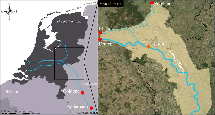
www.nat-hazards-earth-syst-sci.net/19/1895/2019/ Nat. Hazards Earth Syst. Sci., 19, 1895–1908, 20191900 A. Bomers et al.: Decreasing uncertainty in flood frequency analyses Figure 2. Model domain of the 1-D–2-D coupled model. Figure 3. Random input parameters considered in the Monte Carlo analysis. turns out to be between 13 825 and 17 753 m3 s−1 . This large much lower at Lobith compared to the discharge at Ander- reduction in the maximum discharge is caused by the major nach, while the discharges of the other 11 flood events are overflow and dike breaches that occur in present times. Since more or less the same at these two locations (Fig. 4). The re- the 1374 flood event was much larger than the current dis- duction in maximum discharge of the 1374 flood event in the charge capacity of the Lower Rhine, the maximum discharge downstream direction shows the necessity to apply hydraulic at Lobith decreases. The reconstruction of the 1374 flood modelling since the use of a linear regression analysis based over modern topography is presented in detail in Bomers on measured discharges between Cologne and Lobith will et al. (2019b). On the other hand, the other 11 flood events result in an unrealistically larger maximum discharge at Lo- were below this discharge capacity and hence only a slight bith. reduction in discharges was found for some of the events The reconstructed discharges at Lobith are used to extend as a result of dike breaches, whereas overflow did not oc- the systematic data set presented in Fig. 1. In the next sec- cur. Some other events slightly increased as a result of the tion, these discharges are used in an FFA with the use of a inflow of the tributaries Sieg, Ruhr, and Lippe rivers along bootstrap method. the Lower Rhine. This explains why the 1374 flood event is Nat. Hazards Earth Syst. Sci., 19, 1895–1908, 2019 www.nat-hazards-earth-syst-sci.net/19/1895/2019/
A. Bomers et al.: Decreasing uncertainty in flood frequency analyses                                                               1901

Figure 4. Maximum discharges and their 95 % confidence intervals of the reconstructed historic floods at Cologne (Herget and Meurs, 2010)
and simulated maximum discharges and their 95 % confidence intervals at Lobith for the 12 historic flood events.

3    The bootstrap method                                                 The perception threshold is considered to be equal to the
                                                                       discharge of the smallest flood present in the historic period,
The systematic data set covering the period 1772–2019 is ex-           representing the 1535 flood with an expected discharge of
tended with 12 reconstructed historic flood events that oc-            8826 m3 s−1 (Fig. 4). We follow the method of Parkes and
curred in the period 1300–1772. To create a continuous data            Demeritt (2016) assuming that the perception threshold was
set, a bootstrap method based on sampling with replacement             fairly constant over the historical period. However, the max-
is used. The continuous systematic data set (1772–2018) is             imum discharge of the 1535 flood is uncertain and hence the
resampled over the missing years from the start of the his-            perception threshold is also uncertain. Therefore, the percep-
torical period to the start of the systematic record. Two as-          tion threshold is treated as a random uniformly distributed
sumptions must be made such that the bootstrap method can              parameter in the bootstrap method, the boundaries of which
be applied:                                                            are based on the 95 % confidence interval of the 1535 flood
    1. The start of the continuous discharge series since the          event.
       true length of the historical period is not known.                 The bootstrap method consists in creating a continuous
                                                                       discharge series from 1317 to 2018. The method includes the
    2. The perception threshold over which floods were                 following steps (Fig. 5).
       recorded in the historical times before water level and
       discharge measurements were conducted is known.                   1. Combine the 1772–1900 data set with the 1901–2018
                                                                            data set to create a systematic data set.
   Assuming that the historical period starts with the first
known flood (in this study 1342) will significantly underes-             2. Select the flood event with the lowest maximum dis-
timate the true length of this period. This underestimation                 charge present in the historic time period. Randomly
influences the shape of the FF curve (Hirsch and Stedinger,                 sample a value in between the 95 % confidence inter-
1987; Schendel and Thongwichian, 2017). Therefore, Schen-                   val of this lowest flood event. This value is used as the
del and Thongwichian (2017) proposed the following equa-                    perception threshold.
tion to determine the length of the historical period:
                                                                         3. Compute the start of the historical time period (Eq. 2).
       L+N −1
M = L+        ,                                               (2)        4. Of the systematic data set, select all discharges that have
         k
                                                                            an expected value lower than the sampled perception
where M represents the length of the historical period                      threshold.
(years), L the number of years from the first historic flood
to the start of the systematic record (431 years), N the length          5. Use the data set created in Step 4 to create a continuous
of the systematic record (247 years), and k the number of                   discharge series in the historical time period. Randomly
floods exceeding the perception threshold in both the his-                  draw an annual maximum discharge of this systematic
torical period and the systematic record (28 in total). Using               data set for each year within the historical period for
Eq. (2) results in a length of the historical period of 455 years           which no data are available following a bootstrap ap-
(1317–1771).                                                                proach.

www.nat-hazards-earth-syst-sci.net/19/1895/2019/                              Nat. Hazards Earth Syst. Sci., 19, 1895–1908, 2019
1902 A. Bomers et al.: Decreasing uncertainty in flood frequency analyses
We restrict our analysis to the use of a generalized extreme
value (GEV) distribution since this distribution is commonly
used in literature to perform an FFA (Parkes and Demeritt,
2016; Haberlandt and Radtke, 2014; Gaume et al., 2010).
Additionally, several studies have shown the applicability of
this distribution to the flooding regime of the Rhine river
(Toonen, 2015; Chbab et al., 2006; Te Linde et al., 2010). The
GEV distribution has an upper bound and is thus capable of
flattening off at extreme values by having a flexible tail. We
use a bounded distribution since the maximum discharge that
is capable of entering the Netherlands is limited to a physi-
cal maximum value. The crest levels of the dikes along the
Lower Rhine, Germany, are not infinitely high. The height
of the dikes influences the discharge capacity of the Lower
Rhine and hence the discharge that can flow towards Lobith.
Figure 5. Bootstrap method to create a continuous discharge series Using an upper-bounded distribution yields that the FF rela-
in which M represents the length of the historical period and p the tion converges towards a maximum value for extremely large
number of floods exceeding the perception threshold in the histori- return periods. This value represents the maximum discharge
cal period. that is capable of occurring at Lobith.
The GEV distribution is described with the following
equation:
6. Since both the reconstructed as well as the measured ( 1 )
discharges are uncertain due to measurement errors, x −µ ξ
these uncertainties must be included in the analysis. F (x) = exp − ξ , (3)
σ
Therefore, for each discharge present in the systematic
data set and in the historical data set, its value is ran- where (µ) represents the location parameter indicating where
domly sampled based on its 95 % confidence interval. the origin of the distribution is positioned, (σ ) what the scal-
ing parameter describing the spread of the data is, and (ξ )
7. Combine the data sets of Steps 5 and 6 to create a con-
what the shape parameter controlling the skewness and kur-
tinuous data set from 1317 to 2018.
tosis of the distribution is, both influencing the upper tail and
The presented steps in the bootstrap method are repeated hence the upper bound of the system. The maximum like-
5000 times in order to create 5000 continuous discharge data lihood method is used to determine the values of the three
sets resulting in convergence in the FFA. The FFA procedure parameters of the GEV distribution (Stendinger and Cohn,
itself is explained in the next section. 1987; Reis and Stedinger, 2005).
The FFA is performed for each of the 5000 continuous dis-
charge data sets created with the bootstrap method (Sect. 3),
4 Flood frequency analysis resulting in 5000 fitted GEV curves. The average of these
relations is taken to get the final FF curve and its 95 % confi-
An FFA is performed to determine the FF relation of the dif- dence interval. The results are given in the next section.
ferent data sets (e.g. systematic record, historical record). A
probability distribution function is used to fit the annual max-
imum discharges to their probability of occurrence. Many 5 Results
types of distribution functions and goodness-of-fit tests ex-
ist, all with their own properties and drawbacks. However, 5.1 Flood frequency relations
the available goodness-of-fit tests for selecting an appropriate
In this section the FFA results (Fig. 6 and Table 2) of the
distribution function are often inconclusive. This is mainly
following data sets are presented.
because each test is more appropriate for a specific part of the
distribution, while we are interested in the overall fit since the – The 1901 data set measured discharges covering the pe-
safety standards expressed in probability of flooding along riod 1901–2018.
the Dutch dikes vary from 10−2 to 10−5 . Furthermore, we
highlight that we focus on the influence of extending the data – The 1772 data set is as above and extended with the
set of measured discharges on the reduction in uncertainty of data set of Toonen (2015), representing the systematic
the FF relations rather than on the suitability of the different data set and covering the period 1772–2018.
distributions and fitting methods. – The 1317 data set is as above and extended with 12
reconstructed historic discharges and the bootstrap re-
Nat. Hazards Earth Syst. Sci., 19, 1895–1908, 2019 www.nat-hazards-earth-syst-sci.net/19/1895/2019/A. Bomers et al.: Decreasing uncertainty in flood frequency analyses 1903
dicts the lowest values according to the findings of Toonen
(2015). The relatively low positioning of the FF curve con-
structed with the 1772 data, compared to our other 1317 and
1901 data sets, might be explained by the fact that the data
of Toonen (2015) covering the period 1772–1900 have not
been normalized. This period has a relatively high flood in-
tensity (Fig. 1). However, only two flood events exceeded
10 000 m3 s−1 . A lot of dike reinforcements along the Lower
Rhine were executed during the last century. Therefore, it is
likely that before the 20th century, flood events with a max-
imum discharge exceeding 10 000 m3 s−1 resulted in dike
breaches and overflow upstream of Lobith. As a result, the
maximum discharge of such an event decreased significantly.
Although Toonen (2015) mentions that the effect of recent
changes in the river system on discharges of extreme floods
of the Lower Rhine is small, we argue that it does influence
the flood events with maximum discharges slightly lower
than the current main channel and floodplain capacity. Cur-
rently, it is possible for larger floods to flow in the down-
stream direction without the occurrence of inundations com-
pared to the 19th century. Therefore, it is most likely that
the 1772–1900 data set of Toonen (2015) underestimates the
flooding regime of that specific time period influencing the
shape of the FF curve.
5.2 Hypothetical future extreme flood event
After the 1993 and 1995 flood events of the Rhine river, the
FF relation used in Dutch water policy was recalculated tak-
ing into account the discharges of these events. All return
Figure 6. Fitted GEV curves and their 95 % confidence intervals of periods were adjusted. The design discharges with a return
the 1901, 1772, and 1317 data sets. period of 1250 years, which was the most important return
period at that time, was increased by 1000 m3 s−1 (Parmet
et al., 2001). Such an increase in the design discharge re-
sampling method to create a continuous discharge series quires more investments in dike infrastructure and floodplain
covering the period 1317–2018. measures to re-establish the safety levels. Parkes and De-
meritt (2016) found similar results for the river Eden, UK.
If the data set of measured discharges is extended, we find They showed that the inclusion of the 2015 flood event had
a large reduction in the confidence interval of the FF curve a significant effect on the upper tail of the FF curve, even
(Fig. 6 and Table 2). Only extending the data set with the though their data set was extended from 1967 to 1800 by
data of Toonen (2015) reduced this confidence interval by adding 21 reconstructed historic events to the data set of mea-
5200 m3 s−1 for the floods with a return period of 1250 years sured data. Schendel and Thongwichian (2017) argue that if
(Table 2). Adding the reconstructed historic flood events in the flood frequency relation changes after a recent flood, and
combination with a bootstrap method to create a continuous if this change can be ambiguously attributed to this event, the
data set results in an even larger reduction in the confidence data set of measured discharges must be expanded since oth-
interval of 7400 m3 s−1 compared to the results of the 1901 erwise the FF results will be biased upward. Based on their
data set. For the discharges with a return period of 100 000 considerations, it is interesting to see how adding a single
years, we find an even larger reduction in the confidence in- extreme flood event influences the results of our method.
tervals (Table 2). Both the 1317 and 1901 data sets are extended from
Furthermore, we find that using only the 1901 data set 2018 to 2019 with a hypothesized flood in 2019. We as-
results in larger design discharges compared to the two ex- sume that in 2019 a flood event has occurred that equals
tended data sets. This is in line with the work of Toonen the largest measured discharge so far. This corresponds with
(2015). Surprisingly, however, we find that the 1772 data set the 1926 flood event (Fig. 1), having a maximum discharge
predicts the lowest discharges for return periods > 100 years of 12 600 m3 s−1 . No uncertainty of this event is included
(Table 2), while we would expect that the 1317 data set pre- in the analysis. Figure 7 shows that the FF curve based on
www.nat-hazards-earth-syst-sci.net/19/1895/2019/ Nat. Hazards Earth Syst. Sci., 19, 1895–1908, 20191904 A. Bomers et al.: Decreasing uncertainty in flood frequency analyses
Table 2. Discharges (m3 s−1 ) and their 95 % confidence interval corresponding to several return periods for the 1901, 1772, and 1317 data
sets.
Data Q_10 Q_100 Q_1000 2.5 % Q_1250 97.5 % 2.5 % Q_100 000 97.5 %
1901–2018 9264 12 036 14 050 10 594 14 215 20 685 11 301 16 649 29 270
1772-2018 9106 11 442 13 008 11 053 13 130 16 027 11 858 14 813 19 576
1317–2018 8899 11 585 13 655 12 514 13830 15 391 14 424 16 562 19 303
1995 flood events would be less severe if the analysis was
performed with an extended data set as presented in this
study. Consequently, decision makers might have made a dif-
ferent decision since fewer investments were required to cope
with the new flood safety standards. Therefore, we recom-
mend using historical information about the occurrence of
flood events in future flood safety assessments.
6 Discussion
We developed an efficient bootstrap method to include his-
toric flood events in an FFA. We used a 1-D–2-D coupled hy-
draulic model to normalize the data set of Meurs (2006) for
modern topography. An advantage of the proposed method
is that any kind of historical information (e.g. flood marks,
sediment depositions) can be used to extend the data set of
annual maximum discharges as long as the information can
be translated into discharges. Another great advantage of the
proposed method is the computational time to create the con-
tinuous data sets and to fit the GEV distributions. The entire
process is completed within several minutes. Furthermore, it
is easy to update the analysis if more historical information
about flood events becomes available. However, the method
is based on various assumptions and has some drawbacks.
These assumptions and drawbacks are discussed below.
6.1 The added value of normalized historic flood events
The results have shown that extending the systematic data
set with normalized historic flood events can significantly re-
Figure 7. Fitted GEV curves and their 95 % confidence intervals of duce the confidence intervals of the FF curves. This is in line
the 1901 and 1317 data sets if they are extended with a future flood with the work of O’Connell et al. (2002), who claim that the
event. length of the instrumental record is the single most important
factor influencing uncertainties in flood frequency relations.
However, reconstructing historic floods is time-consuming,
especially if these floods are normalized with a hydraulic
the 1901 data set changes significantly as a result of this hy-
model. Therefore, the question arises of whether it is re-
pothesized 2019 flood. We calculate an increase in the dis-
quired to reconstruct historic floods to extend the data set
charge corresponding with a return period of 100 000 years
of measured discharges. Another, less time-consuming, op-
of 1280 m3 s−1 . Contrarily, the 2019 flood has almost no
tion might be to solely resample the measured discharges in
effect on the extended 1317 data set. The discharge corre-
order to extend the length of the data set. Such a method was
sponding to a return period of 100 000 years only increased
applied by Chbab et al. (2006), who resampled 50 years of
slightly by 180 m3 s−1 . Therefore, we conclude that the ex-
weather data to create a data set of 50 000 years of annual
tended data set is more robust to changes in FF relations as
maximum discharges.
a result of future flood events. Hence, we expect that the
changes in FF relations after the occurrence of the 1993 and
Nat. Hazards Earth Syst. Sci., 19, 1895–1908, 2019 www.nat-hazards-earth-syst-sci.net/19/1895/2019/A. Bomers et al.: Decreasing uncertainty in flood frequency analyses 1905
To test the applicability of solely using measured dis-
charges, we use the bootstrap method presented in Sect. 3.
A data set of approximately 700 years (equal to the length
of the 1317 data set) is created based on solely measured
discharges in the period 1901–2018. The perception thresh-
old is assumed to be equal to the lowest measured discharge
such that the entire data set of measured discharges is used
during the bootstrap resampling. Again, 5000 discharge data
sets are created to reach convergence in the FFA. These data
are referred to as the Q_Bootstrap data set.
We find that the use of the Q_Bootstrap data set, based on
solely resampling the measured discharges of the 1901 data
set, results in lower uncertainties of the FF curve compared
to the 1901 data set (Fig. 8). This is because the length of
the measured data set is increased through the resampling
method. Although the confidence interval decreases after re-
sampling, the confidence interval of the Q_Bootstrap data
set is still larger compared to the 1317 data set, including
the normalized historic flood events (Fig. 8). This is because
the variance of the Q_Bootstrap data set, which is equal to
4.19×10⁶ m3 s−1 , is still larger than the variance of the 1317
data set. For the Q_Bootstrap data set, the entire measured
data set (1901–2018) is used for resampling, while for the
1317 data set only the discharges below a certain threshold
in the systematic time period (1772–2018) are used for re-
sampling. The perception threshold was chosen to be equal
to the lowest flood event in the historical time period hav-
ing a discharge of between 6928 and 10724 m3 s−1 . Hence,
the missing years in the historical time period are filled with
relatively low discharges. Hence, the variance of the 1317
data set is relatively low (3.35 × 10⁶ m3 s−1 ). As a result of Figure 8. Fitted GEV curves of the 1901, 1317, and Q_Bootstrap
the lower variance, the uncertainty intervals are also smaller data sets.
compared to the Q_Bootstrap data set.
Furthermore, the FF curve of the Q_Bootstrap data set is
only based on a relatively short data set of measured dis- pling the measured data set, we assume that the flood series
charges and hence only based on the climate conditions of consists of independent and identically distributed random
this period. Extending the data set with historic flood events variables. This might not be the case if climate variability
gives a better representation of the long-term climatic vari- plays a significant role in the considered time period result-
ability in flood events since these events have only been nor- ing in a period of extreme low or high flows. However, up till
malized for changes in the river system and thus still capture now no consistent large-scale climate change signal in ob-
the climate signal. We conclude that reconstructing historic served flood magnitudes has been identified (Blöschl et al.,
events, even if their uncertainty is large, is worth the effort 2017).
since it reduces the uncertainty intervals of design discharges In Sect. 5, we found that extending the data set from 1901
corresponding to rare flood events, which is crucial for flood to 1772 resulted in a shift in the downward direction of the
protection policymaking. FF curve. This is because in the period 1772–1900, a rel-
atively small number of floods exceeded a discharge larger
6.2 Resampling the systematic data set than 10 000 m3 s−1 . Since no large flood events were present
in the period 1772–1900, this data set has a lower variance
The shape of the constructed FF curve strongly depends on compared to the 1901 data set. Using both the 1772 and 1901
the climate conditions of the period considered. If the data set data sets for resampling purposes influences the uncertainty
is extended with a period which only has a small number of of the FF curve. To identify this effect, we compared the re-
large flood events, this will result in a significant shift of the sults if solely the measured discharges (1901–2018) are used
FF curve in the downward direction. This shift can be over- for resampling purposes and if the entire systematic data set
estimated if the absence of large flood events only applies to (1772–2018) period is used. We find that using the entire sys-
the period used to extend the data set. Furthermore, by resam- tematic data set results in a reduction in the 95 % confidence
www.nat-hazards-earth-syst-sci.net/19/1895/2019/ Nat. Hazards Earth Syst. Sci., 19, 1895–1908, 20191906 A. Bomers et al.: Decreasing uncertainty in flood frequency analyses
intervals compared to the situation in which solely the mea- ences the variance of the considered data set and hence the
sured discharges are used caused by the lower variance in the uncertainty of the FF curve. Using a smaller threshold re-
period 1772–1900. However, the reduction is at a maximum sults in an increase in the variance of the data set and hence
of 12 % for a return period of 100 000 years. Although the in an increase in the uncertainty intervals. The proposed as-
lower variance in the 1772–1900 data set might be explained sumption related to the perception threshold can only be used
by the fact that these discharges are not normalized, the lower if there is enough confidence that the smallest known flood
variance may also be caused by the natural variability in cli- event in the historical time is indeed the actual smallest flood
mate. event that occurred in the considered time period.
6.3 Distribution functions and goodness-of-fit tests 6.5 A comparison with Bayesian statistics
In Sect. 5, only the results for a GEV distribution were pre- The FFA was performed based on frequentist statistics. The
sented. We found that the uncertainty interval of the flood maximum likelihood function was used to fit the parameters
event with a return period of 100 000 years was reduced by of the GEV distribution function. However, only point es-
73 % by extending the data set of approximately 120 years timates are computed. To enable uncertainty predictions of
of annual maximum discharges to a data set with a length of the GEV parameter estimates, the maximum likelihood es-
700 years. Performing the analysis with other distributions timator assumes symmetric confidence intervals. This may
yields similar results. A reduction of 60 % is found for the result in an incorrect estimation of the uncertainty, which is
Gumbel distribution and a reduction of 76 % for the Weibull specifically a problem for small sample sizes. For large sam-
distribution. This shows that, although the uncertainty inter- ple sizes, maximum likelihood estimators become unbiased
vals depend on the probability distribution function used, the minimum variance estimators with approximate normal dis-
general conclusion of reduction in uncertainty of the fitted tributions. Contrarily, Bayesian statistics provide the entire
FF curve holds. posterior distributions of the parameter estimates and thus no
However, by only considering a single distribution func- assumptions have to be made. However, a disadvantage of
tion in the analysis, model uncertainty is neglected. One ap- the Bayesian statistics is that the results are influenced by the
proach to manage this uncertainty is to create a composite priors describing the distributions of the parameters (Neppel
distribution of several distributions each allocated a weight- et al., 2010). For future work, we recommend studying how
ing based on how well it fits the available data (Apel et al., uncertainty estimates differ between the proposed bootstrap
2008). Furthermore, the uncertainty related to the use of var- method and a method which relies on Bayesian statistics such
ious goodness-of-fit tests was neglected since only the max- as the study of Reis and Stedinger (2005).
imum likelihood function was used to fit the sample data to Moreover, a disadvantage of the proposed bootstrap ap-
the distribution function. Using a composite distribution and proach is that, by resampling the systematic data set to fill
multiple goodness-of-fit tests will result in an increase in the the gaps in the historical time period, the shape of the flood
uncertainties of FF curves. frequency curve is influenced in the domain corresponding
to events with small return periods (i.e. up to ∼ 100 years
6.4 The length of the extended data set and the corresponding with the length of the 1901 data set). Methods
considered perception threshold presented by Reis and Stedinger (2005) and Wang (1990) use
historical information solely to improve the estimation of the
The measured data set starting at 1901 was extended to 1317. tail of the FF curves, while the systematic part of the curve
However, the extended data set still has limited length com- stays untouched. Table 2 shows the discharges correspond-
pared to the maximum return period of 100 000 years con- ing to a return period of 100 years for both the 1901 data
sidered in Dutch water policy. Preferably, we would like to set and the extended 1317 data set following the bootstrap
have a data set with at least the same length as the maximum method described in Sect. 3. We find that this discharge de-
safety level considered such that extrapolation in FFAs is not creases from 12 036 to 11 585 m3 s−1 by extending the sys-
required anymore. However, the proposed method is a large tematic data set. This decrease in design discharge by 3.7 %
step to decrease uncertainty. indicates that resampling the systematic data set over the his-
Furthermore, the systematic data set was used to create torical time period only has a little effect on the shape of the
a continuous data set using a bootstrap approach. However, flood frequency curve corresponding to small return periods.
preferably we would like to have a continuous historical This finding justifies the use of the bootstrap method.
record since now the low flows are biased on climate con-
ditions of the last 250 years. Using this data set for resam-
pling influences the uncertainty intervals of the FF curves. 7 Conclusions
If the historical climate conditions highly deviated from the
current climate conditions, this approach does not produce Design discharges are commonly determined with the use
a reliable result. In addition, the perception threshold influ- of flood frequency analyses (FFAs) in which measured dis-
Nat. Hazards Earth Syst. Sci., 19, 1895–1908, 2019 www.nat-hazards-earth-syst-sci.net/19/1895/2019/A. Bomers et al.: Decreasing uncertainty in flood frequency analyses 1907
charges are used to fit a probability distribution function. Acknowledgements. This research has benefited from cooperation
However, discharge measurements have been performed only within the network of the Netherlands Centre for River studies,
for the last 50–100 years. This relatively short data set of NCR (https://ncr-web.org/, last access: 15 February 2019).
measured discharges results in large uncertainties in the pre- The authors would like to thank the Dutch Ministry of Infrastruc-
diction of design discharges corresponding to rare events. ture and Water Management, Juergen Herget (University of Bonn),
and Willem Toonen (KU Leuven) for providing the data. Further-
Therefore, this study presents an efficient bootstrap method
more, the authors would like to thank Willem Toonen (KU Leuven)
to include historic flood events in an FFA. The proposed for his valuable suggestions that improved the paper. In addition,
method is efficient in terms of computational time and set- the authors would like to thank Elena Volpi (Roma Tre University)
up. Additionally, the basic principles of the traditional FFA and the two anonymous reviewers for their suggestions during the
remain unchanged. discussion period, which greatly improved the quality of the pa-
The proposed bootstrap method was applied to the dis- per. Finally, the authors would like to thank Bas van der Meulen,
charge series at Lobith. The systematic data set covering Kim Cohen, and Hans Middelkoop from Utrecht University for their
the period 1772–2018 was extended with 12 historic flood cooperation in the NWO project “Floods of the past–Design for the
events. The historic flood events reconstructed by Meurs future”.
(2006) had a large uncertainty range, especially for the most
extreme flood events. The use of a 1-D–2-D coupled hy-
draulic model reduced this uncertainty range of the maxi- Financial support. This research has been supported by the NWO
mum discharge at Lobith for most flood events as a result (project no. 14506), which is partly funded by the Ministry of Eco-
nomic Affairs and Climate Policy. Furthermore, the research is sup-
of the overflow patterns and dike breaches along the Lower
ported by the Ministry of Infrastructure and Water Management and
Rhine. The inclusion of these historic flood events in combi- Deltares.
nation with a bootstrap method to create a continuous data
set resulted in a decrease in the 95 % uncertainty interval
of 72 % for the discharges at Lobith corresponding to a re- Review statement. This paper was edited by Bruno Merz and re-
turn period of 100 000 years. Adding historical information viewed by Elena Volpi and two anonymous referees.
about rare events with a large uncertainty range in combina-
tion with a bootstrap method thus has the potential to signif-
icantly decrease the confidence interval of design discharges
of extreme events.
References
Since correct prediction of flood frequency relations with
little uncertainty is of high importance for future national Apel, H., Merz, B., and Thieken, A. H.: Quantifica-
flood protection programmes, we recommend using histor- tion of uncertainties in flood risk assessments, Interna-
ical information in the FFA. Additionally, extending the data tional Journal of River Basin Management, 6, 149–162,
set with historic events makes the flood frequency relation https://doi.org/10.1080/15715124.2008.9635344, 2008.
less sensitive to future flood events. Finally, we highlight Blöschl, G., Hall, J., Parajka, J., et al.: Changing climate
that the proposed method to include historical discharges in shifts timing of European floods, Science, 357, 588–590,
a traditional FFA can be easily implemented in flood safety https://doi.org/10.1126/science.aan2506, 2017.
assessments because of its simple nature in terms of mathe- Bomers, A., Schielen, R. M. J., and Hulscher, S. J. M. H.:
Consequences of dike breaches and dike overflow in
matical computations as well as its computational efforts.
a bifurcating river system, Nat. Hazards, 97, 309–334,
https://doi.org/10.1007/s11069-019-03643-y, 2019a.
Bomers, A., Schielen, R. M. J., and Hulscher, S. J. M. H.: The severe
Code and data availability. This work relied on data which are 1374 Rhine river flood event in present times, in: 38th IAHR
available from the providers cited in Sect. 2. The code is writ- World Congres, Panama City, Panama, 2019b.
ten for MATLAB, which is available upon request by contacting Bronstert, A., Bardossy, A., Bismuth, C., Buiteveld, H., Disse, M.,
Anouk Bomres (a.bomers@utwente.nl). Engel, H., Fritsch, U., Hundecha, Y., Lammersen, R., Niehoff,
D., and Ritter, N.: Multi-scale modelling of land-use change and
river training effects on floods in the Rhine basin, River Res.
Author contributions. AB, RMJS, and SJMHH contributed towards Appl., 23, 1102–1125, https://doi.org/10.1002/rra.1036, 2007.
the conceptualization of the study. AB set up and carried out the Brunner, G. W.: HEC-RAS, River Analysis System Hydraulic Ref-
methodology and drafted the paper. All co-authors jointly worked erence Manual, Version 5.0, Tech. Rep. February, US Army Corp
on enriching and developing the draft, also in reaction to the review- of Engineers, Hydrologic Engineering Center (HEC), Davis,
ers’ recommendations. USA, available at: https://www.hec.usace.army.mil/software/
hec-ras/documentation/HEC-RAS5.0ReferenceManual.pdf (last
access: 12 March 2019), 2016.
Competing interests. The authors declare that they have no conflict Chbab, E. H., Buiteveld, H., and Diermanse, F.: Estimat-
of interest. ing Exceedance Frequencies of Extreme River Discharges
Using Statistical Methods and Physically Based Approach,
www.nat-hazards-earth-syst-sci.net/19/1895/2019/ Nat. Hazards Earth Syst. Sci., 19, 1895–1908, 2019You can also read