Data Warehouse and Decision Support on Integrated Crop Big Data Vuong M. Ngo
←
→
Page content transcription
If your browser does not render page correctly, please read the page content below
Int. J. Business Process Integration and Management                                                                1

                                                                 Data Warehouse and Decision Support on
                                                                 Integrated Crop Big Data

                                                                 Vuong M. Ngo
                                                                 E-mail: vuong.nm@ou.edu.vn, vuong.ngo@ucd.ie

                                                                 Nhien-An Le-Khac
                                                                 E-mail: an.lekhac@ucd.ie
arXiv:2003.04470v2 [cs.DB] 12 Apr 2021

                                                                 M-Tahar Kechadi
                                                                 E-mail: tahar.kechadi@ucd.ie

                                                                 Ho Chi Minh City Open University, HCMC, Vietnam
                                                                 University College Dublin, Belfield, Dublin 4, Ireland

                                                                 Abstract: In recent years, precision agriculture is becoming very popular. The
                                                                 introduction of modern information and communication technologies for collecting and
                                                                 processing Agricultural data revolutionise the agriculture practises. This has started a
                                                                 while ago (early 20th century) and it is driven by the low cost of collecting data about
                                                                 everything; from information on fields such as seed, soil, fertiliser, pest, to weather data,
                                                                 drones and satellites images. Specially, the agricultural data mining today is considered as
                                                                 Big Data application in terms of volume, variety, velocity and veracity. Hence it leads to
                                                                 challenges in processing vast amounts of complex and diverse information to extract useful
                                                                 knowledge for the farmer, agronomist, and other businesses. It is a key foundation to
                                                                 establishing a crop intelligence platform, which will enable efficient resource management
                                                                 and high quality agronomy decision making and recommendations. In this paper, we
                                                                 designed and implemented a continental level agricultural data warehouse (ADW). ADW
                                                                 is characterised by its (1) flexible schema; (2) data integration from real agricultural
                                                                 multi datasets; (3) data science and business intelligent support; (4) high performance;
                                                                 (5) high storage; (6) security; (7) governance and monitoring; (8) consistency, availability
                                                                 and partition tolerant; (9) cloud compatibility. We also evaluate the performance of ADW
                                                                 and present some complex queries to extract and return necessary knowledge about crop
                                                                 management.

                                                                 Keywords: Data warehouse, decision support, crop Big Data, smart agriculture.

                                                                 Reference to this paper should be made as follows: Ngo, V.M., Le-Khac, N.A. and
                                                                 Kechadi, M.T. (2020) ‘Data Warehouse and Decision Support on Integrated Crop Big
                                                                 Data’, Int. J. Business Process Integration and Management, Vol. 10, No. 1, pp. 17–28.

                                                                 Biographical notes: Vuong M. Ngo received the B.E, M.E and PhD degrees in
                                                                 computer science at HCMC University of Technology in 2004, 2007 and 2013 respectively.
                                                                 He is currently a Senior Researcher at UCD and HCMC Open University. His research
                                                                 interests include information retrieval, sentiment analysis, data mining, graph matching
                                                                 and data

                                                                 Nhien-An Le-Khac is currently a Lecturer at the School of Computer Science, UCD
                                                                 and a Programme Director of MSc programme in forensic computing and cybercrime
                                                                 investigation. He obtained his PhD in computer science in 2006 at the Institut National
                                                                 Polytechnique Grenoble, France. His research interest spans the area of cybersecurity
                                                                 and digital forensics, data mining/distributed data mining for security, grid and high
                                                                 performance computing.

                                                                 M-Tahar Kechadi was awarded PhD and Master degrees in computer science from
                                                                 University of Lille 1, France. He joined the UCD School of Computer Science in 1999.
                                                                 He is currently Professor of Computer Science at UCD. His research interests span the
                                                                 areas of data mining, data analytics, distributed data mining, heterogeneous distributed
                                                                 systems, grid and cloud Computing, cybersecurity, and digital forensics. He is a Principal
                                                                 Investigator at Insight Centre for Data Analytics and CONSUS project. He is a member
                                                                 of IEEE and ACM.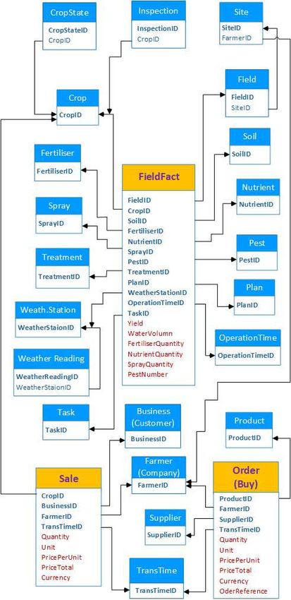
Int. J. Business Process Integration and Management, Vol. 10, No. 1, 2020                                            2

1 Introduction                                              dimensions. The data sources are very diversified and
                                                            varying levels of quality. Precision agriculture (PA)
Annual world cereal productions were 2, 608 million         warehousing has many decision-making processes and
tons and 2, 595 million tons in 2017 and 2018,              each needs different levels of data access and different
respectively (USDA report, 2018; FAO-CSDB report,           needs of analysis. Finally, there are many stakeholders
2018). However, there were also around 124 million          involved in the data ownership and exploitation. So,
people in 51 countries faced food crisis and food           the data has significant number of uncertainties. For
insecurity (FAO-FSIN report, 2018). According to            examples, the quality of data collected by farmers
United Nations (UN document, 2017), we need an              depends directly on their knowledge, routines and
increase 60% of cereal production to meet 9.8 billion       frequency of information recording, and support tools,
people needs by 2050. To satisfy the huge increase          etc. All these issues make the PA data unique when it
demand for food, crop yields must be significantly          becomes to its storage, access, and analysis. These issues
increased using modern farming approaches, such as          may exist in other domains, but not at the same scale
smart farming also called precision agriculture. As         and as in agriculture practices.
highlighted in the European Commission report (EC               In this research, we firstly analyse real-world
report, 2016), precision agriculture is vitally important   agricultural Big Data to build the effective constellation
for the future and can make a significant contribution to   schema. From this schema, some simple questions can be
food security and safety.                                   easily answered directly from the modelled data. These
    The precision agriculture’s current mission is to use   questions include: (1) For a given field, what kind of
the decision-support system (DSS) based on Big Data         crops are suitable to grow? (2) Which companies can
approaches to provide precise information for more          purchase a specific crop with the highest price in the past
control of waste and farming efficiency, such as soil       season? (3) List the history of soil texture and applied
nutrient (Rogovska and et al., 2019), early warning         fertilisers for a given field; (4) List costs of production
(Rembold and et al., 2019), forecasting (Bendre and         for wheat and barley in the last 5 years, and so on.
et al., 2015), irrigation systems (Huang and et al.,        Secondly, the proposed ADW has enough main features
2013), evapotranspiration prediction (Paredes and et al.,   and characteristics of Big Data Warehouse (BDW).
2014), soil and herbicide, insecticide optimisation (Ngo    These are (1) high storage capacity, high performance
and Kechadi, 2020), awareness (Lokers and et al.,           and cloud computing compatibility; (2) flexible schema
2016), supply chain (Protopop and Shanoyan, 2016) and       and integrated storage structure; (3) data ingestion,
financial services (Ruan and et al., 2019). Normally,       monitoring, and security to deal with the data veracity.
the DSSs implement a knowledge discovery process            Besides, an experimental evaluation is conducted to
also called data mining process, which consists of          study the performance of ADW storage.
data collection and data modelling, data warehousing,           The rest of this paper is organised as follows:
data analysis (using machine learning or statistical        in the next Section, we reviewed the related work
techniques), and knowledge deployment (Dicks and            about decision support systems and data warehouses
et al., 2014). Hence, designing and implementing an         in agriculture. In Sections 3, 4 and 5, we presented
efficient agricultural data warehouse (ADW) is one of       big data aspects of PA, our ADW architecture and its
the key steps of this process, as it defines a uniform      modules. In Sections 6, 7, 8 and 9, the quality criteria,
data representation through its schema model and stores     implementation, performance analysis and decision-
the derived datasets so that they can be analysed to        making applications of the proposed ADW are presented
extract useful knowledge. However, currently, this step     respectively. Section 10 gives some concluding remarks
was not given much attention. Therefore, there are very     and future research directions. Finally, a concrete
few reports in the literature that focus on the design      example about the ADW and its operational average
of efficient ADWs with the view to enable Agricultural      run-times are shown in the appendix.
Big Data analytics and mining. The design of large scale
ADWs is very challenging. Because, the agricultural
data is spatial, temporal, complex, heterogeneous, non-     2 Related Work
standardised, high dimensional, collected from multi-
sources, and very large. In particular, it has all the      In precision agriculture, DSSs are designed to support
features of Big Data; volume, variety, velocity and         different stakeholders such as farmers, advisers and
veracity. Moreover, the precision agriculture system can    policymakers to optimise resources, farms’ management
be used by different kinds of users at the same time,       and improve business practices (Gutierreza and et al.,
for instance by farmers, policymakers, agronomists, and     2019). For instance, DSSs were built to 1) manage
so on. Every type of user needs to analyse different        microbial pollution risks in dairy farming (Oliver and
information, sets thus requiring specific analytics.        et al., 2017); 2) analyse nitrogen fertilisation from
    Unlike in any other domains; health-care, financial     satellite images (Lundstrom and Lindblom, 2018); 3)
data, etc, the data and its warehousing in precision        control pest and disease under uncertainty in climate
agriculture are unique. This is because, there are very     conditions (Devitt and et al., 2017); 4) manage drip
complex relationships between the agricultural data         irrigation and its schedule (Friedman and et al., 2016);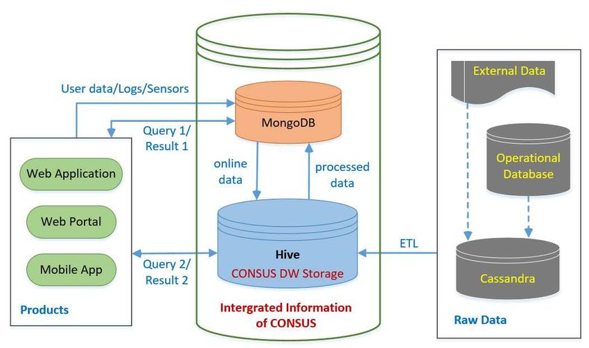
Int. J. Business Process Integration and Management                                                           3

5) predict and adopt climate risks (Han and et al.,           RDF format, and cached in the RDF triple store before
2017). However, the datasets that were used in the            being transformed into relational format. The actual
mentioned studies are small. Besides, they focused            data used for analysis was contained in the relational
on using visualisation techniques to assist end-users         database. However, as the schemas used in Schulze and
understand and interpret their data.                          et al. (2007) and Schuetz and et al. (2018) were based
    Recently, many papers have been published on how          on entity-relationship models, they cannot deal with
to exploit intelligent algorithms on sensor data to           high-performance, which is the key feature of a data
improve agricultural economics Pantazi (2016), Park and       warehouse.
et al. (2016), Hafezalkotob and et al. (2018), Udiasa            In Nilakanta and et al. (2008), a star schema
and et al. (2018) and Rupnik and et al. (2019). In            model was used. All data marts created by the star
Pantazi (2016), the authors predicted crop yield by           schemas are connected via some common dimension
using self-organising-maps; namely supervised Kohonen         tables. However, a star schema is not enough to present
networks, counter-propagation artificial networks and         complex agricultural information and it is difficult
XY-fusion. In Park and et al. (2016), one predicted           to create new data marts for data analytics. The
drought conditions by using three rule-based machine          number of dimensions of the DW proposed in Nilakanta
learning; namely random forest, boosted regression            and et al. (2008) is very small; only 3-dimensions
trees, and Cubist. To select the best olive harvesting        – Species, Location, and Time. Moreover, the DW
machine, the authors in Hafezalkotob and et al. (2018)        concerns livestock farming. Overcoming disadvantages of
applied the target-based techniques on the main criteria,     the star schema, the authors of Ngo and et al. (2018) and
which are cost, vibration, efficiency, suitability, damage,   Ngo and Kechadi (2020) proposed a constellation schema
automation, work capacity, ergonomics, and safety. To         for an agricultural DW architecture in order to satisfy
provide optimal management of nutrients and water,            the quality criteria. However, they did not describe how
the paper Udiasa and et al. (2018) exploited the multi-       to design and implement their DW.
objective genetic algorithm to implement an E-Water
system. This system enhanced food crop production at
river basin level. Finally, in Rupnik and et al. (2019)       3 Crop Big Data
the authors predicted pest population dynamics by using
time series clustering and structural change detection        3.1 Crop Datasets
which detected groups of different pest species. However,
                                                              The datasets were primarily obtained from an agronomy
the proposed solutions are not scalable enough to handle
                                                              company, which extracted it from them operational
agricultural Big Data; they present weaknesses in one
                                                              data storage systems, research results, and field trials.
of the following aspects: data integration, data schema,
                                                              Especially, we were given real-world agricultural datasets
storage capacity, security and performance.
                                                              on iFarms, Business-to-Business (B2B) sites, technology
    From a Big Data point of view, the papers Kamilaris
                                                              centres and demonstration farms. Theses datasets were
and et al. (2018) and Schnase and et al. (2017) have
                                                              collected from several European countries and they are
proposed “smart agricultural frameworks”. In Kamilaris
                                                              presented in Figures 1 and 2 (Origin report, 2018). These
and et al. (2018), the authors used Hive to store and
                                                              datasets describe more than 112 distribution points,
analyse sensor data about land, water and biodiversity
                                                              73 demonstration farms, 32 formulation and processing
which can help increase food production with less
                                                              facilities, 12.7 million hectares of direct farm customer
environmental impact. In Schnase and et al. (2017), the
                                                              footprint and 60, 000 trial units.
authors moved toward a notion of climate analytics-
as-a-service, by building a high-performance analytics
and scalable data management platform, which is based
on modern cloud infrastructures, such as Amazon web
services, Hadoop, and Cloudera. However, the two
papers did not discuss how to build and implement a
DW for a precision agriculture.
    The proposed approach, inspired from Schulze and
et al. (2007), Schuetz and et al. (2018), Nilakanta and
et al. (2008) and Ngo and et al. (2018), introduces
ways of building agricultural data warehouse (ADW). In
Schulze and et al. (2007), the authors extended entity-
relationship concept to model operational and analytical
data; called multi-dimensional entity-relationship model.
They also introduced new representation elements and
showed how can be extended to an analytical schema.
In Schuetz and et al. (2018), a relational database
and an RDF triple store were proposed to model the                    Figure 1: Data from UK and Ireland.
overall datasets. The data is loaded into the DW in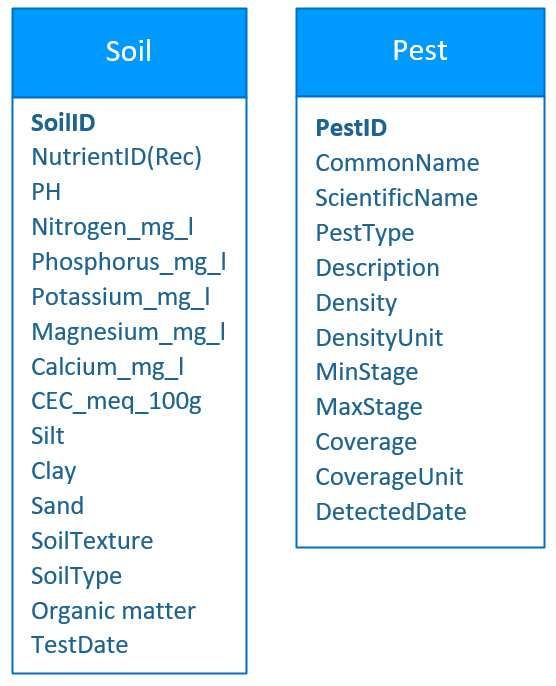
4        Ngo, V.M., Le-Khac, N.A. and Kechadi M.T.

                                                               4. Veracity: The tendency of agronomic data is
                                                                  uncertain, inconsistent, ambiguous and error prone
                                                                  because the data is gathered from heterogeneous
                                                                  sources, sensors and manual processes.

                                                             3.3 ADW Schema

         Figure 2: Data in Continental Europe.

    There is a total of 29 datasets. On average, each
dataset contains 18 tables and is about 1.4 GB
in size. Each dataset focuses on a few information
that impact the crop. For instance, the weather
dataset includes information on location of weather
stations, temperature, rainfall and wind speed over
time. Meanwhile, soil component information in farm
sites, such as mineral, organic matter, air, water and
micro-organisms, were stored in the soil dataset. The
fertiliser dataset contains information about field area
and geographic position, crop name, crop yield, season,
fertiliser name and quantity.

3.2 Big Data Challenges

Raw and semi-processed agricultural datasets are usually
collected through various sources: Internet of Thing
(IoT) devices, sensors, satellites, weather stations,
robots, farm equipment, farmers and agronomists, etc.
Besides, agricultural datasets are very large, complex,
unstructured, heterogeneous, non-standardised, and
inconsistent. Hence, it has all the features of Big Data.

    1. Volume: The amount of agricultural data is
       increasing rapidly and is intensively produced
       by endogenous and exogenous sources. The
       endogenous data is collected from operational
       systems, experimental results, sensors, weather
       stations, satellites, and farming equipment. The
       systems and devices in the agricultural ecosystem
       can be connected through IoT. The exogenous data
       concerns the external sources, such as government
       agencies, retail agronomists, and seed companies.
       They can help with information about local pest
       and disease outbreak tracking, crop monitoring,
       food security, products, prices, and knowledge.

    2. Variety: Agricultural data has many different
       forms and formats, structured and unstructured
       data, video, imagery, chart, metrics, geo-spatial,
       multi-media, model, equation, text, etc.              Figure 3: A part of ADW schema for Precision
                                                             Agriculture
    3. Velocity: The collected data increases at very high
       rate, as sensing and mobile devices are becoming
       more efficient and cheaper. The datasets must be      The DW uses schema to logically describe the entire
       cleaned, aggregated and harmonised in real-time.      datasets. A schema is a collection of objects, including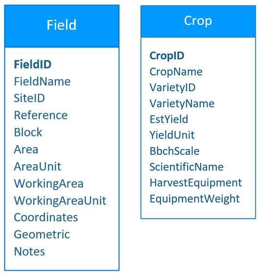
Int. J. Business Process Integration and Management                                                               5

tables, views, indexes, and synonyms which consist            used to support Crop table. While, Site and Weather
of some fact and dimension tables (Oracle document,           Reading tables support Field and WeatherStation tables.
2017). The DW schema can be designed based on the             FieldFact fact table saves the most important facts
model of source data and the user requirements. There         about teh field; yield, water volume, fertiliser quantity,
are three kind of models, namely star, snowflake and          nutrient quantity, spray quantity and pest number.
fact constellation. With the its various uses, the ADW        While, in Order and Sale tables, the important facts
schema needs to have more than one fact table and             needed by farm management are quantity and price.
should be flexible. So, the constellation schema, also
known galaxy schema should be used to design the ADW
schema.
                                                              Table 1    Descriptions of other dimension tables
                                                                      Dim.
                                                                No.                Particular attributes
                                                                      tables
                                                                                   BusinessID, Name, Address, Phone,
                                                                1     Business
                                                                                   Mobile, Email
                                                                                   CropStateID, CropID, StageScale,
                                                                                   Height,     MajorStage,    MinStage,
                                                                2     CropState
                                                                                   MaxStage, Diameter, MinHeight,
                                                                                   MaxHeight, CropCoveragePercent
                                                                                   FarmerID, Name, Address, Phone,
                                                                3     Farmer
                                                                                   Mobile, Email
                                                                                   FertiliserID, Name, Unit, Status,
                                                                4     Fertiliser
                                                                                   Description, GroupName
                                                                                   InspectionID, CropID, Description,
                                                                                   ProblemType, Severity, Problem-
                                                                5     Inspection
                                                                                   Notes, AreaValue, AreaUnit, Order,
                                                                                   Date, Notes, GrowthStage
                                                                                   NutrientID, NutrientName, Date,
      Figure 4: Field and Crop dimension tables                 6     Nutrient
                                                                                   Quantity
                                                                      Operation    OperationTimeID, StartDate, End-
                                                                7
                                                                      Time         Date, Season
                                                                                   PlanID, PName, RegisNo, Product-
                                                                8     Plan         Name, ProductRate, Date, Water-
                                                                                   Volume
                                                                                   ProductID, ProductName, Group-
                                                                9     Product
                                                                                   Name
                                                                                   SiteID,     FarmerID,      SiteName,
                                                                10    Site         Reference, Country, Address, GPS,
                                                                                   CreatedBy
                                                                                   SprayID,        SprayProductName,
                                                                                   ProductRate, Area,Date, WaterVol,
                                                                11    Spray        ConfDuration,       ConfWindSPeed,
                                                                                   ConfDirection, ConfHumidity, Conf-
                                                                                   Temp, ActivityType
                                                                                   SupplierID, Name, ContactName,
                                                                12    Supplier
                                                                                   Address, Phone, Mobile, Email
                                                                                   TaskID, Desc, Status, TaskDate,
                                                                13    Task
                                                                                   TaskInterval, CompDate, AppCode
                                                                      Trans        TransTimeID, OrderDate, Deliver-
                                                                14
       Figure 5: Soil and Pest dimension tables                       Time         Date, ReceivedDate, Season
                                                                                   TreatmentID,        TreatmentName,
    We developed a constellation schema for ADW and                                FormType, LotCode, Rate, Appl-
                                                                15    Treatment
it is partially described in Figure 3. It includes few fact                        Code, LevlNo, Type, Description,
tables and many dimension tables. FieldFact fact table                             ApplDesc, TreatmentComment
contains data about agricultural operations on fields.                             WeatherReadingID,        WeatherSta-
Order and Sale fact tables contain data about farmers’                             tionID, ReadingDate, ReadingTime,
trading operations. The key dimension tables are                      Weather      AirTemperature, Rainfall, SPLite,
                                                                16
                                                                      Reading      RelativeHumidity,        WindSpeed,
connected to their fact table. There are some dimension
                                                                                   WindDirection,     SoilTemperature,
tables connected to more than one fact table, such as
                                                                                   LeafWetness
Crop and Farmer. Besides, CropState, Inspection, Site,                Weather      WeatherStationID,       StationName,
and Weather Reading dimension tables are not connected          17
                                                                      Station      Latitude, Longitude, Region
to any fact table. CropState and Inspection tables are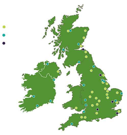
6 Ngo, V.M., Le-Khac, N.A. and Kechadi M.T.
The dimension tables contain details on each instance before it is analysed in the data mining module. A data
of an object involved in a crop yield or farm management. cube is a data structure that allows advanced analysis of
Figure 4 describes attributes of Field and Crop data according to multiple dimensions that define a given
dimension tables. Field table contains information about problem. The data cubes are manipulated by the OLAP
name, area, co-ordinates (being longitude and latitude engine. The DW storage, data mart and data cube are
of the centre point of the field), geometric (being a considered as metadata, which can be applied to the data
collection of points to show the shape of the field) and used to define other data. Finally, Data Mining module
site identify the site that the field it belongs to. While, contains a set of techniques, such as machine learning,
Crop table contains information about name, estimated heuristic, and statistical methods for data analysis and
yield of the crop (estYield), BBCH Growth Stage Index knowledge extraction at multiple level of abstraction.
(BbchScale), harvest equipment and its weight. These
provide useful information for crop harvesting.
Figure 5 describes attributes of Soil and Pest 5 ETL and OLAP
dimension tables. Soil table contains information about
PH value (a measure of the acidity and alkalinity), The ETL module contains Extraction, Transformation,
minerals (nitrogen, phosphorus, potassium, magnesium and Loading tools that can merge heterogeneous
and calcium), its texture (texture label and percentage schemata, extract, cleanse, validate, filter, transform
of Silt, Clay and Sand), cation exchange capacity and prepare the data to be loaded into a DW. The
(CEC) and organic matter. Besides, information about extraction operation allows to read, retrieve raw data
recommended nutrient and testing dates ware also from multiple and different types of data sources systems
included in this table. In Pest table contains name, type, and store it in a temporary staging. During this
density, coverage and detected dates of pests. For the operation, the data goes through multiple checks – detect
remaining dimension tables, their main attributes are and correct corrupted and/or inaccurate records, such
described in Table 1. as duplicate data, missing data, inconsistent values and
wrong values. The transformation operation structures,
converts or enriches the extracted data and presents it
4 ADW Architecture in a specific DW format. The loading operation writes
the transformed data into the DW storage. The ETL
A DW is a federated repository for all the data that implementation is complex, and consuming significant
an enterprise can collect through multiple heterogeneous amount of time and resources. Most DW projects usually
data sources; internal or external. The authors in use existing ETL tools, which are classified into two
Golfarelli and Rizzi (2009) and Inmon (2005) defined groups. The first is a commercial and well-known group
DW as a collection of methods, techniques, and tools and includes tools such as Oracle Data Integrator, SAP
used to conduct data analyses, make decisions and Data Integrator and IBM InfoSphere DataStage. The
improve information resources. DW is defined around second group is famous for it open source tools, such as
key subjects and involves data cleaning, data integration Talend, Pentaho and Apatar.
and data consolidations. Besides, it must show its OLAP is a category of software technology that
evolution over time and is not volatile. provides the insight and understanding of data in
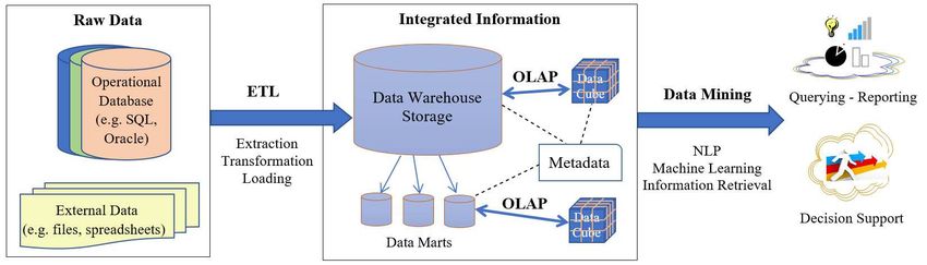
The general architecture of a typical DW system multiple dimensions through fast, consistent, interactive
includes four separate and distinct modules; Raw Data, access, management and analysis of the data. By using
Extraction Transformation Loading (ETL), Integrated roll-up (consolidation), drill-down, slice-dice and pivot
Information and Data Mining (Kimball and Ross, 2013), (rotation) operations, OLAP performs multidimensional
which is illustrated in Figure 6. In that, Raw Data analysis in a wide variety of possible views of information
(source data) module is originally stored in various that provides complex calculations, trend analysis
storage systems (e.g. SQL, sheets, flat files, ...). The and sophisticated data modelling quickly. The OLAP
raw data often requires cleansing, correcting noise and systems are divided into three categories: 1) Relational
outliers, dealing with missing values. Then it needs to be OLAP (ROLAP), which uses relational or extended-
integrated and consolidated before loading it into a DW relational database management system to store and
storage through ETL module. manage the data warehouse; 2) Multidimensional OLAP
The Integrated Information module is a logically (MOLAP), which uses array-based multidimensional
centralised repository, which includes the DW storage, storage engines for multidimensional views of data,
data marts, data cubes and OLAP engine. The DW rather than in a relational database. It often requires
storage is organised, stored and accessed using a suitable pre-processing to create data cubes. 3) Hybrid OLAP
schema defined by the metadata. It can be either (HOLAP), which is a combination of both ROLAP and
directly accessed or used to create data marts, which is MOLAP. It uses both relational and multidimensional
usually oriented to a particular business function or an techniques to inherit the higher scalability of ROLAP
enterprise department. A data mart partially replicates and the faster computation of MOLAP.
DW storage’s contents and is a subset of DW storage. In the context of agricultural Big Data, HOLAP is
Besides, the data is extracted in a form of data cube more suitable than both ROLAP and MOLAP because: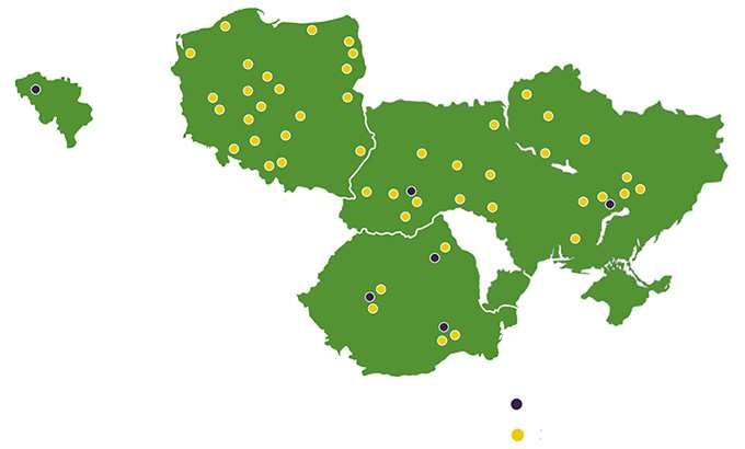
Int. J. Business Process Integration and Management                                                          7

                                Figure 6: Agricultural Data Warehouse Architecture.

1) ROLAP has quite slow performance and does not             and efficient information transaction. In the last
meet all the users’ needs, especially when performing        criterion, a user satisfaction survey should be used to
complex calculations; 2) MOLAP is not capable of             find out how a given DW satisfies its user’s expectations.
handling detailed data and requires all calculations to be
performed during the data cube construction; 3) HOLAP
inherits advantages of both ROLAP and MOLAP, which           7 ADW Implementation
allow the user to store large data volumes of detailed
information and perform complex calculations within          Currently, there are many popular large-scale database
reasonable response time.                                    types that can implement DWs. Redshift (Amazon
                                                             document, 2018), Mesa (Gupta and et al., 2016),
                                                             Cassandra (Hewitt and Carpenter, 2016; Neeraj, 2015),
6 Quality Criteria                                           MongoDB (Chodorow, 2013; Hows and et al., 2015)
                                                             and Hive (Du, 2018; Lam and et al., 2016). In Ngo
The accuracy of data mining and analysis techniques          and et al. (2019), the authors analysed the most
depends on the quality of the DW. As mentioned in            popular no-sql databases, which fulfil most of the
Adelman and Moss (2000) and Kimball and Ross (2013),         aforementioned criteria. The advantages, disadvantages,
to build an efficient ADW, the quality of the DW should      as well as similarities and differences between Cassandra,
meet the following important criteria:                       MongoDB and Hive were investigated carefully in the
                                                             context of ADW. It was reported that Hive is a better
  1. Making information easily accessible.                   choice as it can be paired with MongoDB to implement
                                                             the proposed ADW for the following reasons:
  2. Presenting consistent information.
                                                               1. Hive is based on Hadoop which is the most
  3. Integrating data correctly and completely.                   powerful cloud computing platform for Big Data.
  4. Adapting to change.                                          Besides, HQL is similar to SQL which is popular
                                                                  for the majority of users. Hive supports well
  5. Presenting and providing right information at the            high storage capacity, business intelligent and data
     right time.                                                  science more than MongoDB or Cassandra. These
                                                                  Hive features are useful to implement ADW.
  6. Being a secure bastion         that   protects   the
     information assets.                                       2. Hive does not have real-time performance so it
                                                                  needs to be combined with MongoDB or Cassandra
  7. Serving as the authoritative and trustworthy                 to improve its performance.
     foundation for improved decision making. The
     analytics tools need to provide right information         3. MongoDB is more suitable than Cassandra to
     at the right time.                                           complement Hive because: 1) MongoDB supports
                                                                  joint operation, full text search, ad-hoc query and
  8. Achieving benefits, both tangible and intangible.            second index which are helpful to interact with the
  9. Being accepted by DW users.                                  users. Cassandra does not support these features;
                                                                  2) MongoDB has the same master – slave structure
    The above criteria must be formulated in a                    with Hive that is easy to combine. While the
form of measurements. For example, with the 8th                   structure of Cassandra is peer - to - peer; 3) Hive
criterion, it needs to determine quality indicators about         and MongoDB are more reliable and consistent.
benefits, such as improved fertiliser management, cost            So the combination of both Hive and MongoDB
containment, risk reduction, better or faster decision,           adheres to the CAP theorem.
8 Ngo, V.M., Le-Khac, N.A. and Kechadi M.T.
Figure 7: Agricultural Data Warehouse Implementation
The ADW implementation is illustrated in Figure for testing. Every group has 5 queries and uses one, two
7 which contains three modules, namely Integrated or more commands (see Table 2). Moreover, every query
Information, Products and Raw Data. The Integrated uses operators; And, Or, ≥, Like, Max, Sum and Count,
Information module includes two components; to express complex queries.
MongoDB and Hive. MongoDB receives real-time data;
as user data, logs, sensor data or queries from Products Table 2 Command combinations of queries
module, such as web application, web portal or mobile Group Commands
app. Besides, some results which need to be obtained G1 Where
in real-time will be transferred from the MongoDB to G2 Where, Group by
Products. Hive stores the online data and sends the G3 Where, Left (right) Join
processed data to MongoDB. Some kinds of queries G4 Where, Union
having complex calculations will be sent directly to G5 Where, Order by
Hive. G6 Where, Left (right) Join, Order by
G7 Where, Group by, Having
In the Raw Data module, almost data in Operational
G8 Where, Group by, Having, Order by
Databases or External Data components, is loaded into
G9 Where, Group by, Having, Left (right) Join,
Cassandra. It means that we use Cassandra to represent Order by
raw data storage. Hence, with the diverse formats of G10 Where, Group by, Having, Union, Order by
raw data; image, video, natural language and sql data,
Cassandra is better to store them than SQL databases.
In the idle times of the system, the updated raw data in Group 1
Cassandra will be imported into Hive through the ELT Group 2
Different times (T imesqi )
tool. This improves the performance of ETL and helps 30 Group 3
us deploy ADW on cloud or distributed systems. Group 4
Group 5
20 Group 6
Group 7
8 Performance Analysis Group 8
10 Group 9
The performance analysis was conducted using MySQL Group 10
5.7.22, JDK 1.8.0 171, Hadoop 2.6.5 and Hive 2.3.3
1
which run on Bash, on Ubuntu 16.04.2, and on Windows 0
10. All experiments were run on a desktop with an 0 10 20 30 40 50
Intel Core i7 CPU (2.40 GHz) and 16 GB memory. Queries (qi )
We only evaluate the performance of reading operation
as ADW is used for reporting and data analysis. Figure 8: Different times between MySQL and
The database of ADW is duplicated into MySQL to ADW in runtime of every Query
compare performance. By combining popular HQL/SQL
commands, namely Where, Group by, Having, Left All queries were executed three times and we took
(right) Join, Union and Order by, we created 10 groups the average value of the their execution timess. TheInt. J. Business Process Integration and Management 9
difference in runtime between MySQL and ADW for a of a reading query on MySQL and ADW is 687.8 seconds
query qi is calculated as T imesqi = RTqmysqli
/RTqADW
i
. and 216.1 seconds, respectively. It means that ADW
Where, RTqi mysql
and RTqi ADW
are average runtimes of is faster 3.19 times. In the future, by deploying ADW
query qi on MySQL and ADW, respectively. Moreover, solution on cloud or distributed systems, we believe that
with each group Gi , the difference in runtime between the performance will be even much better than MySQL.
MySQL and ADW is T imesGi = RTGmysql i
/RTGADW
i
.
Where, RTGi = Average(RTqi ) is average runtime of
group Gi on MySQL or ADW. 9 Application for Decision Making
Figure 8 describes the time difference between
MySQL and ADW for every query. Although running on The proposed ADW and study its performance on real
one computer, but with large data volume, ADW is faster agricultural data, we illustrated some queries examples
than MySQL on 46 out of 50 queries. MySQL is faster to show how to extract information from ADW. These
for three queries 12th , 13th and 18th belonging to groups queries incorporate inputs on crop, yield, pest, soil,
3rd and 4th . The two systems returned the same time fertiliser, inspection, farmer, businessman and operation
for query 24th from group 5th . Within each query group, time to reduce labour and fertiliser inputs, farmer
for fair performance comparison, the queries combine services, disease treatment and also increase yields.
randomly fact tables and dimensional tables. This makes These query information could not be extracted if the
complex queries taking more time and the time difference Origin’s separate 29 datasets have not been integrated
is significant. When varying the sizes and structures of into ADW. The data integration through ADW is
the tables, the difference is very significant; see Figure 8. actually improve the value of a crop management data
over time to better decision-making.
Different times (T imesGi )
6.24 Example 1: List fields, crops in the fields, yield and
6 pest in the field with conditions: (1) the fields do not
4.66 4.63 used ’urea’ fertilizer; (2) the crops has ’yellow rust’ or
’brown rust’ diseases; (3) the crops were grown in 2015.
4 3.36
3.19 2.92 3.16
2.86
Mean 2.27
select CR.CropName, FI.FieldName, FF.Yield,
2 1.56 PE.CommonName, FF.PestNumber, PE.Description
1.22 from FieldFact FF, Crop CR, Field FI, Pest PE,
Fertiliser FE, Inspection INS, OperationTime OP
0 2 4 6 8 10 where FF.CropID = CR.CropID and
Groups (Gi )
FF.FieldID = FI.FieldID and
FF.PestID = PE.PestID and
Figure 9: Different times between MySQL and FF.FertiliserID = FE.FertiliserID and
ADW in runtime of every group CR.CropID = INS.CropID and
FF.OperationTimeID = OP.OperationTimeID and
Beside comparing runtime in every query, we aslo FE.FertiliserName ’urea’ and
compare runtime of every group presented in Figure 9. (INS.Description = ’Yellow Rust’ or
Comparing to MySQL, ADW is more than at most (6.24 INS.Description = ’Brown Rust’) and
times) at group 1st which uses only Where command, Year(INS.Date) = ’2015’ and
and at least (1.22 times) at group 3rd which uses Where Year(OP.StartDate) = ’2015’ and
Year(OP.EndDate) = ’2015’
and Joint commands.
1,109.2
Example 2: List farmers and their crop quantities
1,081.5
Average runtimes (seconds)
1,057.3 were sold by Ori Agro company in 08/2016.
1,000 MySQL
790.4776.6 ADW select FA.FarmerID, FA.FarmerName, CR.CropName,
687.8 SF.Unit, SUM(SF.Quantity)
599.7 571.1 from Salefact SF, business BU, farmer FA, crop CR
483
500 where SF.BusinessID = BU.BusinessID and
342.8 366.4
276.4 238
297.9 SF.FarmerID = FA.FarmerID and
228.3 216.1
173.4205.2 143.7 SF.CropID = CR.CropID and
111.7
91.2 94.2
Month(SF.SaleDate) = ’08’ and
0 Year(SF.SaleDate) = ’2016’ and
1 2 3 4 5 6 7 8 9 10 Mean BU.BusinessName = ’Ori Agro’
group by CR.CropName
Groups (Gi )
Figure 10: Average Runtimes of MySQL and Example 3: List Crops and their fertiliser and
ADW in every Groups treatment information. In that, crops were cultivated
and harvested in 2017, Yield > 10 tons/ha and attached
Figure 10 presents the average runtime of the 10 by ’black twitch’ pest. Besides, the soil in field has PH
query groups on MySQL and ADW. Mean, the run time > 6 and Silt10 Ngo, V.M., Le-Khac, N.A. and Kechadi M.T.
Select CR.CropName, FE.FertiliserName, 10 Conclusion and Future Work
FF.FertiliserQuantity, TR.TreatmentName,
TR.Rate, TR.TreatmentComment
In this paper, we presented a schema herein optimised
From FieldFact FF, Crop CR, OperationTime OT,
Soil SO, PEST PE, Fertiliser FE, Treatment TR for the real agricultural datasets that were made
Where FF.CropID = CR.CropID and available to us. The schema been designed as a
FF.OperationTimeID = OT.OperationTimeID and constellation so it is flexible to adapt to other
FF.SoildID = SO.SoilID and agricultural datasets and quality criteria of agricultural
FF.PestID = PE.PestID and Big Data. Based on some existing popular open source
FF.FertiliserID = FE.FertiliserID and DWs, We designed and implemented the agricultural
FF.TreatmentID = TR.TreatmentID and DW by combining Hive, MongoDB and Cassandra
Year(OT.StartDate) = ’2017’ and DWs to exploit their advantages and overcome their
Year(OT.EndDate) = ’2017’ and limitations. ADW includes necessary modules to deal
FF.Yield > 10 and
with large scale and efficient analytics for agricultural
SO.PH > 6 and SO.SiltInt. J. Business Process Integration and Management 11
WHERE fieldfact.cropid = crop.cropid and
2,297
fieldfact.sprayquantity = 8 and
Average runtimes (seconds)
2,188.4
MySQL crop.EstYield >= 1 and crop.EstYield 100;
1,192
1,000 892.4 8) The query 40th belongs to the group 8th :
754.8
479 422.6 439.5 472.1
SELECT crop.cropname,
233.2 226.7 265.9 212.3 sum(fieldfact.fertiliserquantity) as sum1
97.9 52.7 95.4
3 3.6 5.2 7.6 FROM fieldfact, crop
0
WHERE fieldfact.cropid = crop.cropid and
fieldfact.nutrientquantity= 5 and
5 10 15 20 25 30 35 40 45 50
crop.EstYield 30
Figure 11: Average runtimes of MySQL and ORDER BY crop.cropname;
ADW in 10 typical queries
9) The query 45th belongs to the group 9th :
th rd
3) The query 15 belongs to the group 3 : SELECT nutrient.NutrientName,
SELECT fieldfact.yield, sum(nutrient.Quantity) as sum1
fertiliser.fertiliserName, FROM fieldfact
fertiliser.fertiliserGroupName LEFT JOIN nutrient on
FROM fieldfact fieldfact.NutrientID = nutrient.NutrientID
RIGHT JOIN fertiliser on WHERE nutrient.nutrientName like ’%tr%’ and
fieldfact.fertiliserID = fertiliser.fertiliserID (fieldfact.pestnumber = 16 or
WHERE fieldfact.fertiliserQuantity = 10 and fieldfact.pestnumber = 15)
fertiliser.fertiliserName like ’%slurry%’; GROUP by nutrient.NutrientName
HAVING sum1 5 and sum(fieldfact.watervolumn) as sum1
fieldfact.watervolumn < 20 FROM fieldfact, spray
UNION WHERE fieldfact.sprayid = spray.sprayid and
SELECT productname fieldfact.Yield > 4 and fieldfact.Yield < 8
FROM product, orderfact GROUP by sprayproductname
WHERE product.ProductID = orderfact.ProductID HAVING sum1 > 210
and (orderfact.Quantity = 5 or UNION
orderfact.Quantity = 6); SELECT productname as name1,
sum(orderfact.Quantity) as sum2
5) The query 25th belongs to the group 5th : FROM product, orderfact
SELECT fieldfact.fieldID, field.FieldName, WHERE product.ProductID = orderfact.ProductID and
field.FieldGPS, spray.SprayProductName (orderfact.Quantity = 5 or
FROM fieldfact, field, spray orderfact.Quantity = 6)
WHERE fieldfact.FieldID = field.FieldID and GROUP by productname
fieldfact.SprayID = spray.SprayID and HAVING sum2 > 50
fieldfact.PestNumber = 6 ORDER BY name1;
ORDER BY field.FieldName;
6) The query 30th belongs to the group 6th :
Acknowledgment
SELECT fieldfact.FieldID, nutrient.NutrientName,
nutrient.Quantity, nutrient.‘Year‘ This research is an extended work of Ngo and et al.
FROM fieldfact (2019) being part of the CONSUS research program. It is
RIGHT JOIN nutrient on funded under the SFI Strategic Partnerships Programme
fieldfact.NutrientID = nutrient.NutrientID (16/SPP/3296) and is co-funded by Origin Enterprises Plc.
WHERE fieldfact.NutrientQuantity = 3 and
fieldfact.fertiliserquantity = 3
ORDER BY nutrient.NutrientName References
LIMIT 10000;
Adelman, S. and Moss, L. (2000). Data warehouse project
7) The query 35th belongs to the group 7th :
management, 1st edition. Addison-Wesley Professional.
SELECT crop.cropname,
sum(fieldfact.watervolumn) as sum1 Amazon document (2018). Amazon Redshift database
FROM fieldfact, crop developer guide. Samurai ML.12 Ngo, V.M., Le-Khac, N.A. and Kechadi M.T.
Bendre, M. R. and et al. (2015). Big data in precision Hewitt, E. and Carpenter, J. (2016). Cassandra: the definitive
agriculture: Weather forecasting for future farming. In guide, 2nd edition (distributed data at web scale). O’Reilly
International Conference on Next Generation Computing Media.
Technologies (NGCT). IEEE.
Hows, D. and et al. (2015). The definitive guide to MongoDB,
Cao, T. and et al. (2012). Semantic search by latent 3rd edition (a complete guide to dealing with big data using
ontological features. International Journal of New MongoDB. Apress.
Generation Computing, Springer, SCI, 30(1):53–71.
Huang, Y. and et al. (2013). Estimation of cotton yield
Chodorow, K. (2013). MongoDB: The definitive guide, 2nd with varied irrigation and nitrogen treatments using
edition (powerful and scalable data storage). O’Reilly aerial multispectral imagery. International Journal of
Media. Agricultural and Biological Engineering, 6(2):37–41.
Inmon, W. H. (2005). Building the data warehouse. Wiley.
Devitt, S. K. and et al. (2017). A cognitive decision tool to
optimise integrated weed management. In Proceedings of Kamilaris, A. and et al. (2018). Estimating the environmental
International Tri-Conference for Precision Agriculture. impact of agriculture by means of geospatial and big data
analysis: the case of Catalonia, pages 39–48. Springer.
Dicks, L. V. and et al. (2014). Organising evidence for
environmental management decisions: a ‘4s’ hierarchy. Kimball, R. and Ross, M. (2013). The data warehouse toolkit:
Trends in Ecology & Evolution, 29(11):607–613. the definitive guide to dimensional modeling (3rd edition).
Wiley.
Du, D. (2018). Apache Hive essentials, 2nd edition. Packt
Publishing. Lam, C. P. and et al. (2016). Hadoop in action, 2nd edition.
Manning.
EC report (2016). Europeans, agriculture and the common
Lokers, R. and et al. (2016). Analysis of big data technologies
agricultural policy. Special Eurobarometer 440, The
for use in agro-environmental science. Environmental
European Commission.
Modelling & Software, 48:494–504.
FAO-CSDB report (2018). Global cereal production and Lundstrom, C. and Lindblom, J. (2018). Considering farmers’
inventories to decline but overall supplies remain adequate,
situated knowledge of using agricultural decision support
release date: December 06, 2018. Cereal Supply and
systems (agridss) to foster farming practices: the case of
Demand Brief, FAO. cropsat. Agricultural Systems, 159:9–20.
FAO-FSIN report (2018). Global report on food crises 2018. Neeraj, N. (2015). Mastering Apache Cassandra, 2nd edition.
Food Security Information Network, FAO. Packt Publishing.
Friedman, S. P. and et al. (2016). Didas – user-friendly Ngo, V. (2014). Discovering latent information by spreading
software package for assisting drip irrigation design and activation algorithm for document retrieval. International
scheduling. Computers and Electronics in Agriculture, Journal of Artificial Intelligence & Applications, 5(1):23–
120:36–52. 34.
Golfarelli, M. and Rizzi, S. (2009). Data warehouse Ngo, V. and et al. (2011). Discovering latent concepts and
design: modern principles and methodologies. McGraw-Hill exploiting ontological features for semantic text search.
Education. In In the 5th Int. Joint Conference on Natural Languag
Processing, ACL, pages 571–579.
Gupta, A. and et al. (2016). Mesa: a geo-replicated
online data warehouse for google’s advertising system. Ngo, V. and et al. (2018). An efficient data warehouse for crop
Communications of the ACM, 59(7):117–125. yield prediction. In The 14th International Conference
Precision Agriculture (ICPA-2018), pages 3:1–3:12.
Gutierreza, F. and et al. (2019). A review of visualisations in
Ngo, V. M. and et al. (2019). Designing and implementing
agricultural decision support systems: An HCI perspective.
data warehouse for agricultural big data. In The 8th
Computers and Electronics in Agriculture, 163.
International Congress on BigData (BigData-2019), pages
Hafezalkotob, A. and et al. (2018). A decision support 1–17. Springer-LNCS, Vol. 11514.
system for agricultural machines and equipment selection: Ngo, V. M. and Kechadi, M. T. (2020). Crop knowledge
A case study on olive harvester machines. Computers and discovery based on agricultural big data integration. In
Electronics in Agriculture, 148:207–216. The 4th International Conference on Machine Learning
and Soft Computing (ICMLSC), pages 1–5. ACM.
Han, E. and et al. (2017). Climate-agriculture-modeling and
decision tool (camdt): a software framework for climate Nilakanta, S. and et al. (2008). Dimensional issues in
risk management in agriculture. Environmental Modelling agricultural data warehouse designs. Computers and
& Software, 95:102–114. Electronics in Agriculture, 60(2):263–278.
Helmer, S. and et al. (2015). A similarity measure for weaving Oliver, D. M. and et al. (2017). Design of a decision support
patterns in textiles. In In the 38th ACM SIGIR Conference tool for visualising e. coli risk on agricultural land using
on Research and Development in Information Retrieval, a stakeholder-driven approach. Land Use Policy, 66:227–
pages 163–172. 234.Int. J. Business Process Integration and Management 13 Oracle document (2017). Database data warehousing guide. Oracle12c doc release 1. Origin report (2018). Annual report and accounts. Origin Enterprises plc. Pantazi, X. E. (2016). Wheat yield prediction using machine learning and advanced sensing techniques. Computers and Electronics in Agriculture, 121:57–65. Paredes, P. and et al. (2014). Partitioning evapotranspiration, yield prediction and economic returns of maize under various irrigation management strategies. Agricultural Water Management, 135:27–39. Park, S. and et al. (2016). Drought assessment and monitoring through blending of multi-sensor indices using machine learning approaches for different climate regions. Agricultural and Forest Meteorology, 216:157–169. Protopop, I. and Shanoyan, A. (2016). Big data and smallholder farmers: Big data applications in the agri-food supply chain in developing countries. International Food and Agribusiness Management Review, IFAMA, 19(A):1– 18. Rembold, F. and et al. (2019). Asap: A new global early warning system to detect anomaly hot spots of agricultural production for food security analysis. Agricultural Systems, 168:247–257. Rogovska, N. and et al. (2019). Development of field mobile soil nitrate sensor technology to facilitate precision fertilizer management. Precision Agriculture, 20(1):40–55. Ruan, J. and et al. (2019). A life cycle framework of green iot-based agriculture and its finance, operation, and management issues. IEEE Communications Magazine, 57(3):90–96. Rupnik, R. and et al. (2019). Agrodss: a decision support system for agriculture and farming. Computers and Electronics in Agriculture, 161:260–271. Schnase, J. and et al. (2017). Merra analytic services: meeting the big data challenges of climate science through cloud-enabled climate analytics-as-a-service. Computers, Environment and Urban Systems, 161:198–211. Schuetz, C. G. and et al. (2018). Building an active semantic data warehouse for precision dairy farming. Organizational Computing and Electronic Commerce, 28(2):122–141. Schulze, C. and et al. (2007). Data modelling for precision dairy farming within the competitive field of operational and analytical tasks. Computers and Electronics in Agriculture, 59(1-2):39–55. Udiasa, A. and et al. (2018). A decision support tool to enhance agricultural growth in the mékrou river basin (west africa). Computers and Electronics in Agriculture, 154:467––481. UN document (2017). World population projected to reach 9.8 billion in 2050, and 11.2 billion in 2100. Department of Economic and Social Affairs, United Nations. USDA report (2018). World agricultural supply and demand estimates 08/2018. United States Department of Agriculture.
You can also read