The Rate of Return on Real Estate: Long-Run Micro-Level Evidence - eCommons@Cornell
←
→
Page content transcription
If your browser does not render page correctly, please read the page content below

The Rate of Return on Real Estate:
                     Long-Run Micro-Level Evidence∗

           David Chambers†                Christophe Spaenjers‡                  Eva Steiner§
       University of Cambridge                    HEC Paris                   Cornell University

                                                June 2019

                                                Abstract

       We provide evidence that direct real estate investments are less proftable and more risky
       in the long run than previously thought. We hand-collect property-level data on realized in-
       come, expenses, and transaction prices from the archives of four large institutional investors
       in the U.K.—historically important Oxbridge colleges—for the period 1901–1970. Gross
       income yields mostly fuctuate around 5%, but trend to lower (higher) levels for agricultural
       and residential (commercial) real estate near the end of our sample period. Operating costs
       mean that net yields are about one third lower than gross yields on average. Long-term
       real income growth rates are between -1.0% and 0.0% for the three main property types.
       Together these fndings imply limited long-run capital gains and real annualized net total
       returns of less than 4% across all property types. Moreover, we fnd substantial volatility
       in net income streams and variation in relative price levels across transacted properties,
       revealing the considerable idiosyncratic risks associated with real estate investments.
       .
       JEL Classification: G11, G12, G23, N20, R30.
       Keywords: real estate, property prices, rental yields, long-run returns, idiosyncratic risks.

   ∗
      We would like to thank David Klingle for excellent research assistance, and Elroy Dimson, William
Goetzmann, Rowena Gray, Dmitry Kuvshinov, Thies Lindenthal, Robert Margo, Ludovic Phalippou, Geert
Rouwenhorst, Moritz Schularick, Johannes Stroebel, Stijn Van Nieuwerburgh, Joachim Voth, Guillaume
Vuillemey, and seminar and conference participants at HEC Paris, London School of Economics, University of
Geneva, and the World Economic History Congress 2018 for valuable feedback and data. We are grateful to the
Cambridge Endowment for Research in Finance, the Centre for Endowment Asset Management, the Newton
Trust, and St John’s College, Cambridge for research funding. All errors are ours.
    †
      Cambridge Judge Business School. Email: d.chambers@jbs.cam.ac.uk.
    ‡
      HEC Paris. Email: spaenjers@hec.fr.
    §
      Cornell SC Johnson College of Business. Email: ems457@cornell.edu.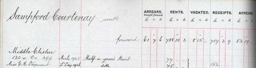
1       Introduction

Real estate has delivered attractive investment returns over the past few decades (e.g., Favilukis
et al. (2017), Ghent et al. (2018), Giglio et al. (2018)).1 Yet, we possess only a limited understand-
ing of its longer-term track record, especially when compared to our knowledge of historical bond
and equity returns (e.g., Jorion and Goetzmann (1999), Dimson et al. (2002)). Recent research
by Jordà et al. (2019a) suggests that residential real estate has been a stellar investment in a wide
sample of advanced economies since the late nineteenth century. It estimates an average real net
return to housing of about 7% per year, similar to equities. However, measuring the historical
performance of direct real estate investments based on existing data sets is an exercise that
is severely complicated by di˙erent data limitations and methodological challenges, at least up
until the 1960s or 1970s. First, available price data typically do not allow for an adequate adjust-
ment for variation in property characteristics. Increases in average prices may thus overstate the

capital gains realized by investors if more recently traded properties are of higher average quality.
Second, information on the cashfows associated with historical real estate investments is diÿcult
to obtain. When income data exist, they capture contractual (instead of realized) income, and
are not drawn from the same set of properties for which transaction prices are observed. Third,
detailed data on the costs associated with real estate ownership are typically not available.
        In this paper, we overcome these measurement problems, which are presented more formally
in Section 2, by exploiting a unique empirical setting where we observe not only transaction
prices but also rental income and costs for the same sample of individual properties. More
specifcally, we construct a data set of the holdings and transactions starting from the early
twentieth century for King’s College and Trinity College in Cambridge and Christ Church and
New College in Oxford. These four prominent colleges were among the wealthiest and most
substantial property owners in each university around 1900. Importantly, the data set is not
restricted to housing, but also includes agricultural and commercial real estate. The latter two
    1
    Favilukis et al. (2017) estimate average real returns to U.S. housing of 9–10%, before maintenance costs
and property taxes, over the 1976–2012 period. For U.K. housing, Giglio et al. (2018) document average real
net returns of about 7% over the 1988–2016 period. Ghent et al. (2018) report average nominal returns to
privately held commercial real estate of 9–12% for di˙erent periods since the 1970s.

                                                     1
property types have received less attention in prior literature despite their importance in the
real estate portfolios of institutional investors. Furthermore, the micro-level nature of this data
allows us to analyze the idiosyncratic risks faced by direct property investors.
Our data cover the period 1901–1970 and are hand-collected from the archives of the
four sample colleges. We obtain data on acquisitions and disposals from transaction ledgers
and source data on rental income and costs from rent books. We match transactions to the
corresponding income records based on property address, tenant name, and other identifying
characteristics. In the case of the two Cambridge colleges, archival sources enable us to assemble
the full history of rental income across all property holdings for the entire sample period. For
the two Oxford colleges, the available records allow us to collect income data for transacted
properties for the periods immediately following purchases and preceding sales. Our fnal data
set contains more than 48,000 income observations at the property-year level, and we observe
a purchase or sale for nearly 2,000 property-year combinations.
The granular data contained in the college archives allow us to analyze all three major
types of real estate; namely, agricultural, residential, and commercial. We frst analyze our
newly-constructed data set by studying the evolution of real estate portfolios across those three
major property types over time. At the start of the twentieth century, both King’s and Trinity’s
portfolios were heavily concentrated in agricultural real estate, which generated more than
three-quarters of total gross income. Over the course of the sample period, we document a shift
away from agricultural real estate in favor of commercial real estate, which by 1970 is by far
the most important property type held by gross income generated. This fnding underlines the
importance for institutional investors of property types other than housing.
Next, we construct quality-adjusted rental income indices over the 1901–1970 period. Our
indices capture the growth in realized income of the property holdings of institutional investors,
rather than the growth in average or aggregate contractual rental income in the economy.
This distinction is important because market-wide income may increase as new higher-quality
properties are added to the existing stock, while the income for any previously-constructed
property may not change in the same way. We document that nominal income remains nearly
2constant over the frst half of the twentieth century and begins to increase from 1945 at an
average rate of 4.6% per year. Real income growth exhibits substantial cyclicality, mirroring
infation and defation patterns in the U.K. economy. Crucially, we show that real income has
not increased over time; estimated annualized growth rates are 0.0% for agricultural, -0.8% for
commercial, and -1.0% for residential real estate. These results imply that any positive capital
gains for institutional investors in U.K. property over much of the twentieth century must have
been driven by income yield compression.
We estimate gross yields associated with real estate transactions by dividing the annual gross
income associated with a property by its transaction price. When measured over moving fve-
year intervals and across property types, the mean income yield fuctuates between 4% and 6%;
the long-run average is close to 5%. Average yields are particularly high—implying low relative
price levels—in the early 1930s and particularly low—implying high relative prices—just before
WWI and near the end of our sample period. We dig deeper into our fndings and break down
the evolution of yields by property type. Our estimates suggest that the yields of residential,
commercial, and agricultural properties are similar until WWII. After 1945, they start to diverge,
with yields for agricultural and residential real estate declining, and yields for commercial real
estate increasing. Our results highlight that inferences drawn about the performance of real estate
as an asset class based on empirical evidence from housing properties alone can be misleading.
When considering the cross-sectional variation in gross yields, we see that there is on average
a di˙erence of 3 percentage points between the frst and the third quartile in the yield distribution
per fve-year period, even in times when the di˙erent property types have comparable average
yields. A regression with a number of transaction-level covariates and fxed e˙ects for property
type, college identifer, geographical region, and transaction year leaves 80% of the variation in
gross yields unexplained. Our estimates imply that some properties will generate signifcantly less
(or more) income than expected; others are likely to sell for considerably less (or more) than an-
ticipated. This fnding highlights the importance of idiosyncratic risks in real estate investment.
Next, we analyze the holding costs associated with real estate investing. Averaging across
years and property types, we estimate a mean cost-to-income ratio of 35%. Commercial real
3estate is associated with somewhat lower average costs, in particular during the fnal decades
of our sample. In aggregate, improvements represent the largest cost category, especially from
the mid-twentieth century onwards. At the level of individual properties, we document that
the impact of costs increases the volatility in property-level net income streams relative to the
volatility of gross income streams. For a given property-year, the probability of a drop in net
income of 10% or more exceeds 20%, which is more than twice as high as for gross income. Our
result implies that ignoring the impact of costs may lead to a substantial underestimation of
the riskiness of real estate investments.
Our results on net income and yield dynamics imply limited long-run capital gains, and
annualized real net total returns of less than 4% for the di˙erent property types. For housing,
our estimate is substantially below previous results based on aggregate income and price
statistics—often with incomplete quality adjustments—from disparate sources, even for the
same geography and time period. The di˙erence mainly lies in the income component of the
return to investment. We fnd an average net income yield of 2.8% for U.K. residential real estate
over the 1901-1970 period, while Jordà et al. (2019a) estimate an average yield of 4.1% over the
same time interval. We show that this discrepancy is related to very di˙erent income growth
estimates for the two decades following the start of WWII—a period over which the aggregate
rent data underlying Jordà et al. (2019a) are thin. In sum, our results indicate that real estate
may be a poorer long-term investment than the existing academic literature on housing suggests.
The remainder of this paper is structured as follows. In the next section, we introduce a
defnition of total returns, review the measurement problems in prior research, and explain how
we overcome those methodological issues. Section 3 presents the empirical setting and describes
our data collection, the resulting data sets, and summary statistics. Section 4 presents our
main fndings on portfolio dynamics, income growth, yields, costs, capital gains, and net total
returns. The fnal two sections discuss these results and conclude, respectively.
42 Measuring the Returns to Real Estate Investments
2.1 Return Defnitions
To understand the nature of direct property investments, we present a decomposition of total
returns. We begin by defning the total return to holding property i between time t − 1 and
t, net of the costs associated with property ownership, as:
Pi,t + (1 − ci,t )Yi,t
ri,t = − 1, (1)
Pi,t−1
where Pi,t denotes the market value of property i at time t. While Pi,t is not continuously
∗
observable, it can be proxied by the transaction price Pi,t if a transaction takes place at time t.
Yi,t is gross rental income and ci,t is the cost-to-income ratio for property i at time t, respectively.
We can decompose ri,t from Eq. (1) into its constituent elements, namely net income yield
and capital gain, as follows:
Pi,t h Pi,t−1 (1 − ci,t )Yi,t i
ri,t = × 1+ × −1
Pi,t−1 Pi,t Pi,t−1
Pi,t h (1 − ci,t )Yi,t i
= × 1+ −1
Pi,t−1 Pi,t
h i
= (1 + ki,t ) × 1 + (1 − ci,t )yi,t − 1, (2)
|{z} | {z }
capital gain net income yield
where ki,t and yi,t are the capital gain and the gross rental yield of property i as observed
in year t, respectively. Eq. (2) can be expressed in nominal or in real terms; accounting for
infation a˙ects the computation of the capital gain between t − 1 and t (i.e., ki,t ), but not the
measurement of the income yield at time t (i.e., yi,t ). The total return rη,t to property type
η (i.e., agricultural, commercial, or residential) can then be computed as the value-weighted
average total return over all assets i = 1, 2, ..., N in property type η at time t − 1.
52.2 Measurement Problems in Prior Literature
The existing literature on the long-term fnancial characteristics of real estate investments
mainly focuses on housing. Also, most existing work estimates a time series of average capital
gains kη,t , and only less frequently of average total returns rη,t . Guided by the decomposition
of the net total returns to individual property investments shown in Eq. (2), we can summarize
the measurement problems faced by prior long-run studies estimating the performance of real
estate based on historical data as follows:
Capital gains. Many studies document the historical evolution of aggregate house price in-
∗
dices, based on average transaction values Pη,t observed in di˙erent housing markets. Important
contributions include Eichholtz (1997) for Amsterdam, Shiller (2000) for twenty cities in the
U.S., and Knoll et al. (2017) for fourteen di˙erent countries. However, a time series of changes in
∗
Pη,t
average observed transaction prices ∗
Pη,t−1
overestimates the average capital gains kη,t realized by
investors if it does not adequately control for changes in the quality composition of the traded real
estate stock. In particular, if new properties are, on average, of higher quality than existing ones,
then average transaction prices will increase at a rate that exceeds the capital gains of existing
investors. This is a well-known problem encountered in empirical studies of housing price trends.
For example, the U.K. house price index of Knoll et al. (2017) “does not control for quality changes
prior to 1969” (appendix p. 114); more generally, those authors acknowledge that “accurate mea-
surement of quality-adjustments remains a challenge” (p. 342). Next, investors will only realize
capital gains in line with a quality-adjusted price index if they properly maintain their property;
however, such expenditures are often ignored by the literature, as we discuss in more detail below.
Finally, there exists a “superstar city bias” in that many historical studies—even of “national”
housing prices—focus on capitals and other large cities (Dimson et al., 2018), which are known
to have had a higher-than-average rate of price appreciation historically (Gyourko et al., 2013).
Gross income yields and total returns. Modern fnancial institutions invest in real estate
expressly in pursuit of high rental yields (Hudson-Wilson et al., 2005). However, existing
6empirical studies on the investment performance of real estate largely ignore the rental yield
component of total returns. Rental yields are absent from prior research in part because data on
the cashfows from real estate investments are diÿcult to obtain. Unlike transaction prices, rental
income observations are not systematically or centrally recorded. Furthermore, existing data
capture contractual rental income, which can be signifcantly higher than realized income due
to rent arrears and temporary voids, and thus lead to overstated rental yields. Moreover, where
income data are available for property samples, transaction prices are not typically observed for
the same properties. As a result, empiricists often combine income and price data from di˙erent
sources to estimate yields and total returns. For example, Nicholas and Scherbina (2013) add
survey data on contractual rents from 54 income-producing local properties to their price index
estimated over a di˙erent property sample to compute total returns to Manhattan real estate in-
vestments between 1920 and 1939. Brounen et al. (2014) combine the long-run Amsterdam price
index from Eichholtz (1997) with the rent index from a di˙erent set of properties constructed
by Eichholtz et al. (2012) to estimate total returns. Most recently, Jordà et al. (2019a) provide
total return estimates on housing for fourteen countries by combining price indices from Knoll
et al. (2017) and rental income indices estimated from aggregate national statistics in Knoll
(2017). However, all such methods introduce a measurement error in the resulting time series of
income yield estimates if the underlying price and rent observations are obtained from properties
with di˙erent (quality) characteristics (Eichholtz et al., 2018). Moreover, using mismatched
historical income and price change estimates to extrapolate backward from a contemporary
rent-to-price ratio over long periods of time, as in Brounen et al. (2014) and Jordà et al. (2019a),
carries the risk of compounding measurement errors over time (Dimson et al., 2018).
Costs. Prior studies on the investment income earned from real estate holdings typically ignore
the infuence of costs associated with owning and operating real property. For instance, Eichholtz
et al. (2012) document the evolution of marked-to-market rents—not net income—in Amsterdam.
Where existing studies do account for costs, they rely on small samples of aggregate ratios. Jordà
et al. (2019a) attempt to account for the historical costs of property ownership by anchoring their
7estimation to a contemporary aggregate net income yield estimate. Critically, in this literature
the actual asset-level costs of owning and operating real estate—which have to be borne by the
investor and thus materially a˙ect the net income generated by real property—are unobserved.
Furthermore, by focusing on aggregate capital gains or total returns in the housing market,
much of the literature ignores two important dimensions that are particularly relevant for
institutional investors:
Idiosyncratic risks. The return on an individual property ri,t may be substantially above
or below the aggregate return for its property type rη,t for di˙erent reasons. First, price
appreciation rates may vary across regions, quality categories, etc. Second, “transaction-specifc
risk” is non-negligible: if property i transacts in year t, this may happen at a particularly
∗
low or high price Pi,t that is di˙erent from the (unobservable) Pi,t . The idea that in illiquid
asset markets there exists a transaction-specifc idiosyncratic risk component, which may make
observed prices deviate from their expected values, dates back to at least Shiller and Case
(1987).2 Third, for any given property and in any given year, the gross income Yi,t may be
lower than anticipated (i.e., contracted) or costs ci,t may exceed expectations for that year.
This last source of idiosyncratic risk—and in particular the possibility that annual returns may
be volatile because of variation in expenses—has not been explored in prior literature. For
example, the discussion of idiosyncratic risks as a potential explanation for the “housing risk
premium puzzle” in Jordà et al. (2019b) focuses on individual house price volatility.
Property types other than housing. The global real estate market overall is worth $228
trillion; 74% is residential, 14% is commercial, and the remainder is agricultural land and
forestry (Tostevin, 2017). However, only one third of residential property is investable, compared
to two thirds of commercial.3 As a result, housing does not begin to represent the investable
2
Recent literature on this topic includes Sagi (2018) and Giacoletti (2019) for real estate and Lovo and
Spaenjers (2018) for art.
3
Most residential real estate is held by entities, operators, and owner-occupiers whose main purpose is not
investment. In the U.S.—the largest institutional real estate market worldwide—16% of the housing stock
is institutionally owned (U.S. Department of Housing and Urban Development, 2015), compared to 78% of
8opportunity set for institutional real estate investors. It is therefore problematic to draw
inferences about the investment performance of real estate from the performance of residential
property alone. Outside of housing, scholars have studied U.K. agricultural prices (Jadevicius
et al., 2018), and commercial property prices in Manhattan (Wheaton et al., 2009) and in the
U.K. (Scott, 1996). However, these studies either focus on a narrow geography or a limited
number of property types, have a small sample, or lack income data.
2.3 This Paper
In our hand-collected data set, which we will present in Section 3, we directly observe transaction
∗
prices (Pi,t ), income (Yi,t ), and costs across individual properties of di˙erent types. We can
thus compute the cost ratio (ci,t ) in every year, and measure the gross income yield (yi,t ) if the
property transacts in year t. We do not observe an estimate of the property’s market value
Pi,t if it does not trade. However, we can mitigate measurement problems arising from missing
market values by further re-arranging Eq. (2) as follows:
Yi,t yi,t−1 h i
ri,t = × × 1 + (1 − ci,t )yi,t − 1
Yi,t−1 yi,t
yi,t−1 h i
= (1 + gi,t )× × 1 + (1 − ci,t )yi,t − 1, (3)
|{z} yi,t | {z }
income growth | {z } net income yield
yield change
where gi,t denotes the property-level income growth rate between t − 1 and t. Assuming that
∗
average yields on observed transactions yη,t are representative for the asset class in that period,
we can thus compute a property category’s net total return from the observed aggregate income
growth rates, changes in gross income yields, and aggregate cost ratios as follows:
∗
yη,t−1 h
∗
i
rη,t = (1 + gη,t ) × ∗
× 1 + (1 − cη,t )yη,t − 1. (4)
yη,t
commercial real estate (Ling and Archer, 2018). In the U.K., the second-largest institutional real estate market,
4 percent of the £6,000 billion housing stock is held by institutions; in contrast, institutions invest over twelve
times that amount, or £490 billion, in U.K. commercial property (Mitchell, 2017).
9Eq. (4) highlights the importance of income growth in long-term real estate returns. Absent
(future) income growth, price increases will imply higher capital gains today, but lower income
yields going forward. Absent relative price (i.e., yield) changes, capital gains will equal real
income growth rates. Given that in the very long run the average annual yield change cannot
be too di˙erent from zero—yields cannot increase or decrease ad infnitum—we can expect
long-run average capital gains to be relatively close to long-run average income growth rates.
The relationships described in Eq. (4) suggest that accurately measuring rental income
growth rates over time is a prerequisite for a meaningful analysis of long-term real estate returns.
As discussed before in the context of yield estimation, some prior studies construct market-level
housing rent indices. However, as with price indices, adequately controlling for changes in the
quality mix of properties over time remains a challenge. The issue may be particularly relevant
when indices are based on aggregate national statistics, such as for example in Knoll (2017),
who mainly relies on the rent component of cost-of-living and consumer price indices. In a
recent contribution, Eichholtz et al. (2018) explicitly tackle the issue of quality adjustments
using new historical data and conclude that “most of the increase in housing expenditure that
did occur is attributable to increasing housing quality rather than rising rent”.4
3 Data
3.1 Empirical Setting
Our data set is drawn from the real estate investments held by some of the most prominent
Oxford and Cambridge (Oxbridge) colleges. U.K. institutional investors have a long record
of investing in real estate, and the oldest Oxbridge college endowments have held property
for at least fve centuries. For example, King Henry VIII founded Trinity College, Cambridge,
and Christ Church, Oxford, in 1546 and conferred on both colleges an expansive agricultural
4
Note that income from ownership of a fxed set of properties may increase even more slowly than the
quality-adjusted average rental income in the broader economy. This would be the case if the income associated
with a property tends to jump when ownership changes, or if newly leased properties have higher average rents
even after adjusting for their higher quality. Such scenarios are not unlikely if there exist constraints on the
ability of owners to update rents, for example through legal or contractual limits on rent reviews.
10real estate portfolio. At the start of the twentieth century, their portfolios consisted almost
exclusively of real estate (Chambers et al., 2013).5 Notwithstanding diversifcation into stocks
and bonds in the twentieth century, the oldest and wealthiest of the Oxbridge colleges still
allocate over 40% of their endowment to real estate today (Cambridge Associates, 2018).
By the early decades of the twentieth century, the investment and property portfolios of
Oxbridge colleges were being professionally managed. The senior bursar—equivalent to the chief
fnancial oÿcer and chief investment oÿcer rolled into one—of a college was expected (with the
help of professional advice) to set investment strategy, and to execute that strategy in buying
and selling both real estate and fnancial securities. This is particularly apparent in the cases of
Trinity and King’s College in Cambridge (Nicholas (1960), Neild (2008), Chambers et al. (2013)).
3.2 Data Collection
We study King’s College, Cambridge (founded in 1441), and Trinity College, Cambridge, as well
as Christ Church and New College, Oxford (all founded in 1379). These colleges are among the
oldest and wealthiest Oxbridge colleges at the beginning of the twentieth century (Dunbabin,
1975). We begin our data collection in 1901 and end in 1970. We start in 1901 for two reasons.
First, prior to the late nineteenth century, colleges were forbidden by statute from freely buying
or selling property and were restricted in their ability to raise rents and develop their estates
(Neild, 2008). Second, by the turn of the century, benefcial leases charging below-market rents
had been eradicated and all properties were let at market rent (Dunbabin, 1975). The year
1970 is a natural stopping point for our analysis as higher-quality estimates on the performance
of real estate exist from the 1970s onward. Moreover, access to archival records is restricted
after this date, due to the ongoing commercial sensitivity of the data.
We focus on the investment properties held in college endowments and ignore operational
properties outside the endowments, which are typically not for sale and are not let at market
rents. We compile an unbalanced panel data set of property-year observations on rental income
5
In contrast, the largest U.S. university endowments allocated only 10% of their assets to direct real estate
in the early twentieth century (Goetzmann et al., 2010). U.S. institutional investors did not in general begin to
make a substantial allocation to real estate until the 1970s and 1980s (Eagle, 2013)
11received, costs incurred, and transaction values realized, alongside a number of property and
transaction characteristics, as follows.6
For King’s College, Cambridge, we collect annual property-level realized rental income and
costs incurred over the years 1901–1970 from the annual volumes of the so-called “Mundum
Books”. Transactions of properties over the same period are found in the “Ledger Books”. We
record transaction type (purchase or sale), transaction amount, and year. These records further
allow us to identify partial transactions (part of a property) and portfolio sales (more than one
property), as well as instances where the use of the property has changed—often agricultural
land being sold with a permission for residential development. Where available, we collect
information on location, size, and other characteristics of the property. We manually match
income and cost records on the one hand with transaction records on the other hand by the
common property name.
Figure 1 presents an example of a matched transaction for King’s College. Subfgures 1A
and 1B show the income and cost record for a farm property called “Middle Cliston” located in
the village Sampford Courtenay in the county of Devon. In the fnancial year 1926, the property
generated a rental income of £152 in two semi-annual payments, while the costs (including for
“ironmongery” and a “carpenter”) amounted to slightly more than £19 in total. Subfgure 1C
shows part of the document recording the transaction for the same property, which was sold
in 1927 for £2,552.
Figure 1 about here.
6
A few general points about our data collection are worth mentioning. First, for all colleges, we exclude non-
standard rent types such as rentcharges, wayleaves, and contracts related to trust estates. Second, where a cost
record relates to a group of properties (e.g., a row of houses on the same street), we split these costs equally across
the properties. Third, both for King’s and Trinity College, some properties show substantially lower income in
1926; for Trinity we also observe a temporary jump in income in 1925 for some properties. These patterns seem
related to changes in the accounting methods adopted by those colleges. Appendix B explains how we treat the
income records for these years. Fourth, across all colleges, the recorded transaction year may not coincide with the
frst or last calendar year for which we record an income or cost observation. One reason is that a property may
be vacant for some months (or even years) leading up to a sale or remain vacant for some time after it has been
purchased by a college. In such cases, we match the transaction to the last or frst available income observation.
Fifth, it is possible for all colleges to acquire and dispose of properties through means other than purchases
and sales (e.g., through bequests and exchanges). Our records do not capture such acquisitions or dispositions.
12For Trinity College, Cambridge, we collect annual realized property-level rental income
and costs incurred from the Rent Books over the period 1901–1970. Unfortunately, due to a
missing volume in the archives, records are missing for most residential properties for the period
1966–1970. Unlike at King’s, annual income and cost data is reported by tenant name, instead
of property name. When several tenants occupy a property, we aggregate income across all
tenants in the property in a given year. We collect data on transactions over the same period
from the “Sealed Books”. Transactions are reported by property name. Matching tenant-level
income data with property-level transaction data is challenging because there is no one-to-one
relation between the property on which the college receives rent from a tenant and the property
transacted. As a result, we match the Trinity income and transaction records by identifying
unique property characteristics. For both Cambridge colleges, we match in excess of 50% of
the recorded transactions to properties in the income and cost data.
For Christ Church and New College in Oxford, there are some gaps in the archival records,
particularly with respect to rents, due to volumes being destroyed or lost. For these two colleges,
we collect data on transactions over the period 1901–1970.7 We then collect income and cost data
for the year of the transaction and, in case of a sale (purchase), two years before (after). We also
obtain information on contractual income—in addition to realized income—which is available for
certain years. In case of missing records for realized income, we use contractual income whenever
possible. Data on transactions, annual property-level realized and contractual rental income as
well as costs incurred are obtained from the sources outlined in Appendix A, which also outlines
the exact years for which realized and contractual income records are available. Properties are
identifed by name in all sources, allowing us to match income and cost as well as transaction
records. Property and transaction characteristics are collected from all sources as available.
7
On occasion the transaction records include a property, such as a large piece of farmland or a residential
property with multiple tenants, which is sold not in a single transaction but in a series of transactions in the
same year. In particular, Christ Church owned a large number of residential properties in Kentish Town which
were highly homogeneous, earned similar rents and were transacted in close succession at similar prices. In
such instances, we merge all related transactions into a single transaction with a unique identifer and aggregate
all the associated rental income streams into one.
133.3 Resulting Data Sets and Descriptive Statistics
The data collection described above produces two data sets. First, a larger database of 48,613
annual property-level observations on income, cost and property characteristics, mainly based on
records from King’s and Trinity College. The unit of observation is thus a unique property-year
combination, i.e., property i in year t. The data cover 2,949 di˙erent properties.8 Second, a
smaller database of 1,972 matches between the just-mentioned income data and the transaction
records, which will be used in our estimation and analysis of income yields. This database
includes income and cost data as well as corresponding property and transaction characteristics.
Here the unit of observation is a property-transaction combination, i.e., the purchase or sale
of property i in transaction x. (Every transaction is of course associated with a certain year
t.) Our matched property records correspond to 1,542 distinct transactions.
Table 1 shows a number of di˙erent frequency tables for the income database. More specif-
ically, it shows the number of property-year income and cost observations—and the number
of distinct properties that these observations relate to—by decade (Panel A), by college and
property type (Panel B), and by region of the U.K. (Panel C). Our data are spread evenly over
time with an average of approximately 7,000 property-year observations per decade. Based
on the qualitative descriptions provided in the archival records, we classify properties into one
of four main types. We maintain a property’s initial classifcation throughout its life in the
sample. “Agricultural” refers to land used for farming and represents approximately 50% of
the sample. “Commercial” refers to any property let to a retail, industrial or other commercial
business and represents 13% of our income observations. “Residential” refers to any residential
property or building and contributes about 33% of the data.9 “Other”—by far the smallest
category representing 4% of the sample—refers to schools, government buildings, etc. For the
Oxford colleges, our focus on years surrounding transactions of course implies much smaller
8
This is after accounting for the fact that properties sometimes undergo structural changes, e.g. a large
agricultural property may be subdivided into smaller parcels, or a number of smaller parcels may be merged
into a larger property. In such cases, we assign new property identifers when the change occurs.
9
Properties with mixed uses are classifed as much as possible under one of the three main types, with
priority given to agricultural and otherwise to commercial. Where the necessary information is not available,
mixed-use properties are classifed under the “other” category.
14data samples. Table 1 also shows that the Oxbridge colleges were diversifed geographically,
although the largest portfolio shares were located in the East and South of England.
Table 1 about here.
Table 2 reports on the composition of our sample of matched property-transaction obser-
vations. It thus shows the availability of income observations as does Table 1, but we now only
consider property-year combinations matched to a transaction. Observed and matched property
sales outnumber purchases by a factor of almost 3:1.10 Panels A–C summarize the distribution
of matched property-transaction records by purchase and sale over time, by college, and by
property type. We observe the highest trading volume in agricultural real estate, particularly in
terms of sales. The fnal column in each panel shows the number of distinct transactions, which
may comprise multiple transacted properties (due to portfolio transactions), corresponding to
each row. In Panel D, we show the distribution of matched property-transaction observations
over transactions of one (complete) property, partial transactions, and portfolio transactions
of multiple properties. For portfolio transactions, the number of distinct transactions is by
construction lower than the number of property-transaction combinations.
Table 2 about here.
Table 3 provides summary statistics on nominal and real income and transaction prices over
time. We use infation data from Dimson et al. (2019) to convert nominal values into real terms.
In Panel A, we report for each decade the number of non-missing gross income and net income
(i.e., income less costs) observations, together with means and medians. In real terms, both
mean gross and net income decreased substantially after the frst decade of the twentieth century,
but increased in later decades. However, median real income only bottomed out in the 1960s. In
Panel B, we show for each decade the mean and median purchase and sale price levels. In this
panel, the unit of observation is a transaction, not a property-transaction combination, so there
is no double-counting of portfolio transactions. Mean purchase prices are substantially higher
10
However, note that the colleges may have acquired properties through other methods than outright market
purchases.
15than sale prices in all decades. Although mean prices are somewhat higher at the end of our
sample period than in the beginning, there exists no monotonic trend over our sample period.
Table 3 about here.
4 Results
4.1 The Evolution of Real Estate Portfolios
We start our empirical analysis by studying the evolution of the property portfolios of King’s
and Trinity College, for which we have a near-complete history of holdings and associated rental
income. Figure 2 graphs the evolution of the two portfolios. Subfgures 2A and 2B show the time-
series of the number of income-generating properties by property type for both colleges. Subfg-
ures 2C–2F display the evolution of nominal and real (infated to year-1970 British pounds) gross
income along the same dimensions, while subfgures 2G–2J repeat the exercise for net income.
Figure 2 about here.
As can be clearly seen, the portfolios of these institutions have always encompassed all three
property types. At the start of the twentieth century, both colleges were heavily concentrated
in agricultural real estate, which generated more than three-quarters of total gross income. This
allocation refects the nature of their original endowments centuries earlier and a lack of trading
over the intervening period. Yet, from the little that is known of other institutional property
portfolios at the start of the twentieth century, a heavy portfolio allocation towards agricultural
real estate was not unusual (Dunbabin, 1975). Subsequently, over our sample period there was
a signifcant shift for both colleges in portfolio holdings—both in terms of number of properties
and total rental income—away from agricultural real estate in favor of commercial real estate.
So much so that by 1970 commercial is by far the most important property type held by both
institutions. The growing importance of commercial real estate is most striking when studying
the evolution of income rather than the number of properties; average income is of course much
higher for a commercial property than for a residential house. Our fndings underscore the need
16to include property types other than housing in order to produce an accurate estimation of
the long run performance of the entire real estate asset class.
4.2 Gross income growth over time
In the previous subsection we see that aggregate rental income by property type shifts over
time at least in part due to the fuctuations in the number of properties in the college portfolios.
As a result, average property quality is changing from year to year. In order to estimate
quality-controlled (gross) income indices over our sample period, we proceed as follows. In
every year t, we consider all Cambridge properties that are present in our income database
both in year t − 1 and in year t.11 Next, we compute for every year t the percentage change
in aggregate income. Finally, we chain-link the estimated time-series of income growth rates.
The resulting index thus explicitly controls for changes in the quality mix of the portfolio of
properties over time, in a way similar to repeat-sales regressions in the estimation of capital
gains on properties.12
Figure 3 presents the resulting indices, both at the aggregate level and for each of the three
main property types separately. Subfgure 3A shows the nominal indices, while Subfgure 3B
depicts the defated indices alongside annual infation rates. Note that as reported in Panel C of
Table 1, the property portfolios of the two Cambridge colleges are well-diversifed geographically
across the English regions with signifcant exposure to the economically more prosperous South.
As a result, the annual time-series of their combined rental income is broadly representative
of the overall U.K. real estate market.
Figure 3 about here.
Subfgure 3A shows that nominal income remained almost constant over the frst four
decades of our sample period and only starts to increase after WWII. After correcting for
11
To avoid mis-measurement of income trends due to properties that have just entered or are about to exit
the portfolio, we exclude from the analysis any properties for which we observe a transaction between t − 2 and
t + 1, and properties that frst appear in the data set in t − 2 or t − 1 or last appear in the data set in t or t + 1.
12
To interpret the resulting rental income index as a constant-quality one, we of course need to assume that
the expenditures on repairs and maintenance—which we will analyze later—are suÿcient to avoid property
degradation.
17infation, Subfgure 3B presents a very di˙erent picture where real income growth exhibits
substantial time-series variation. First, real rental income decreased dramatically for all property
types during WWI and until 1920, and then rebounded in the early 1920s. This refects the
impact of high infation during the war and its immediate aftermath followed by subsequent
price defation induced by a policy of returning the pound sterling to the gold standard. Second,
residential income continued to grow until the early 1930s, but income for all property types
decreased in the second half of the 1930s, as infation started to rise again. Third, between 1940
and 1970, we see very little real income growth, except for agricultural real estate in the 1960s.13
Table 5 presents annualized nominal (in Panel A) and real (in Panel B) income growth
rates over our complete sample period 1901–1970, and three di˙erent subperiods: pre-WWI,
1914–1945, and post-WWII. As noted before, nominal income grew fast after WWII; the average
growth rate when considering the complete portfolios is 4.6%. Yet, the equivalent number
in real terms is only 0.6%. Considering the full sample period, we estimate that real income
growth is close to zero for all property types. The annualized real growth rates computed based
on the indices shown in Subfgure 3B are 0.0% for agricultural, -0.8% for commercial, and -1.0%
for residential real estate. These results imply that the colleges can have achieved capital gains
in excess of infation on their real estate investments only if gross income yields declined.
Table 5 about here.
4.3 Gross Income Yields
We now turn to estimating gross income yields from our data set, based on the matched
transactions–rental income database. We exclude “other” property types, furnished lettings,
partial transactions, and small transactions defned as below £500 in year-1970 terms (about
£5,500 at the end of 2018). For a property bought (sold) in year t, we use the maximum
real income generated by the property over the calendar years t until t + 2 (t − 2 until t).
We consider these two-year windows before (after) a disposition (acquisition) to minimize the
13
Rent controls may have held back rental income growth over certain parts of our sample period (e.g.,
1915–1923, 1939–1957) (Knoll, 2017).
18e˙ect of temporary voids on income and present an income estimate that is representative for
the stabilized operation of a given property. (For instance, properties may be vacated by the
occupants prior to a disposition. Alternatively, there may be an initial lease-up period just
after the completion of an acquisition.) We exclude cases where this maximum equals zero.
We then divide real income by the real transaction price. For portfolio transactions (i.e., a
set of properties purchased or sold by one of our colleges in a single transaction), we observe
the transaction price for the entire portfolio. To compute yields on portfolio transactions, we
aggregate income over all properties reported as being bought or sold in the same transaction.
We then classify the transaction under a single property type (agricultural, commercial, or
residential) according to the property in the portfolio that generates the highest income in the
year of the transaction. We winsorize our yield estimates at the 5th and 95th percentile.
Panel A of Table 6 presents summary statistics for the gross income yields estimated over
the same subperiods shown in Table 5. We fnd equal-weighted (value-weighted) mean yields
before costs of 4.1%–5.4% (3.4%–5.2%). Panels B–D of Table 6 repeat the same exercise for
each of the main property types, separately. The relatively low yields for residential real estate
and relatively high yields for commercial real estate after WWII are particularly striking.
Table 6 about here.
Subfgure 4A provides summary statistics for the estimated income yields (equal-weighted
and value-weighted mean, median, frst and third quartile), measured over moving fve-year
periods. We are showing the statistics over moving intervals as the samples can get small in any
given individual year, especially in the early decades of our sample time frame. In most periods,
the mean gross income yields are between 4% and 6%. Taking a simple average over all periods,
we fnd a value of 4.7% for the equal-weighted mean yields (4.8% for the value-weighted mean
yields). Our estimates suggest that mean yields exceed 6% in the 1930s, a period during which
defation caused a temporary increase in real rental income (cf. Figure 3). By contrast, the
results reported indicate that mean yields drop below 4% before WWI and revert to the same
levels near the end of our sample period.
19Figure 4 about here.
Subfgure 4B presents equal-weighted means by property type over moving ten-year periods.
The mean yields average to 4.7% for agricultural, 5.7% for commercial, and 4.5% for residential
real estate over all periods. Our estimated yields for the di˙erent property types move in a
narrow range until WWII. Thereafter, yields for agricultural and residential real estate trend
downwards, while yields for commercial real estate trend in the opposite direction. As Figure
3 depicted, real income for residential properties in the 1960s was in line with previous decades,
while agricultural properties exhibited substantial income growth in the same decade. The
lower yields at the end of the sample period thus point to signifcant real price rises for these
property types. By contrast, the increasing yields on commercial real estate in the last two
decades of our sample period imply substantial real price decreases then.
Our granular data on income and transaction prices allow us to document cross-sectional
variation in realized yields across individual real estate assets and the di˙erent property types.
For example, Subfgure 4A exhibits an average di˙erence of about 3 percentage points between
the frst and the third quartiles of income yields for all properties, even in times when the
di˙erent property types have comparable average yields. This fnding highlights the importance
of idiosyncratic risks in real estate investments. First, some properties will generate less income
than expected. Second, at the time of purchase and sale, the prices for some properties will
be lower or higher than anticipated.
Table 7 presents output from a regression with transaction-level yields as the dependent
variable, estimated as a function of property and transaction characteristics. The results
reported suggest that purchases (rather than sales), portfolio transactions, and commercial
properties are associated with higher yields, i.e., lower prices relative to the income stream.
We estimate that a change in use around the time of a sale, which typically represents an
agricultural property that can now be developed for residential or commercial use, is correlated
with lower yields, i.e., a higher relative price. Despite the inclusion of a comprehensive set of
covariates, as well as fxed e˙ects for college identity, geographical region, and transaction time,
the R2 of the regression is only 20.0%, implying that a large proportion of the total variation in
20yields remains unexplained. These regression results reinforce the importance of idiosyncratic
risk factors in the pricing of real estate investment assets.
Table 7 about here.
4.4 The Impact of Costs
In what follows, we analyze the extent to which costs reduce realized income yields. The college
rent books show that the di˙erent types of cost incurred in managing their properties, namely,
repairs, improvements, property taxes and rates, payments to estate agents or brokers, and
insurance. To assess their importance, we compare costs and realized income aggregated across
the two Cambridge colleges. Subfgure 5A displays the results both aggregated over all properties
and by property type. When considering the average across years for all property types, we
document a mean cost-to-income ratio of 35%. In many years the ratio ranges between 30%
and 40%, but we document substantial variation outside this range. Commercial real estate is
associated with the lowest average cost ratio (28.2%), especially in the fnal decades of the study
period. Residential (36.7%) and especially agricultural real estate (43.4%) have higher relative
costs, meaning that net yields will deviate more from gross yields for these property types.
Figure 5 about here.
For Trinity College, we have annual rent book summaries that allow us to break down total
costs into di˙erent categories. We show the results in Subfgure 5B. Improvements represent
the largest cost category, especially after World War II.
Figure 5 focuses on aggregate costs. However, there exists substantial variation across
properties and over time in the extent to which costs depress net income. The upshot is that
property-level net income streams will be much more volatile than gross income streams. This
fnding is illustrated in Figure 6. We show for every year the distribution of property-level gross
or net income changes over the prior year across fve categories: a decrease of 10% or more,
a decrease of less than 10%, no change, an increase of less than 10%, or an increase of 10%
or more. Subfgure 6A points to the relative stability of gross income streams; sharp decreases
21or increases are relatively uncommon. However, in Subfgure 6B, we see a completely di˙erent
story when taking into account costs. When pooling data across years, we estimate that the
probability of a property-level decrease in net income of 10% or more (and of an increase
in net income of 10% or more) exceeds 20%. Ignoring costs therefore leads to a substantial
underestimation of the volatility of real estate income streams and thus total net returns.
Figure 6 about here.
4.5 Capital Gains and Net Total Returns
Our fndings allow us to estimate capital gains and the net total rate of return on real estate.
First consider housing. We have documented an average income yield of 4.5% over the sample
period, with an average cost-to-income ratio of 36.7%. These estimates imply an average net
income yield of about 2.8%. Following Section 2, the total real capital gain implied by the start
and end values of both the real income index (shown in Subfgure 3B) and the gross yield series
can be computed as follows:
∗
yη,1901
kη,1901→1970 = (1 + gη,1901→1970 ) × ∗
− 1. (5)
yη,1970
We use the frst (last) available decade-level average yield from Subfgure 4B as a proxy for
∗ ∗
yη,1901 (yη,1970 ). If we then annualize the total capital gain given by Eq. (5), we fnd a geometric
average rate of real price appreciation of 0.2% between 1901 and 1970 for residential real estate.
Our estimate of the annualized real net total return to housing over our sample period is thus
approximately 3.0%. Table 8 presents our estimated decomposition of the annualized net total
returns for each of residential, agricultural and commercial real estate. (For commercial real
estate, the initial yield is computed starting in 1911.) In the case of the latter two property
types, we document annualized net total returns of 3.8% and 2.3% in real terms, respectively.
Table 8 about here.
Over the same time period 1901–1970, annualized real total returns to U.K. government
bonds and equities were 0.1% and 5.0%, respectively, according to Dimson et al. (2019). The
22performance of real estate thus falls in between these two more traditional assets. Dimson et al.
(2011) perform a decomposition of long-run equity returns for the period 1900-2010 similar in
spirit to ours. The mean total real equity return for 19 countries largely arises from the average
dividend yield over the sample period, with the real dividend growth rate slightly below zero
on average and a modest contribution from the decline in dividend yields (rise in valuations)
over time. We observe a qualitatively similar decomposition in our real estate returns analysis,
especially for agricultural and residential real estate.
5 Discussion
Our study is the frst to provide a property-type specifc breakdown of total returns to real
estate investments in the long run. Our estimates suggest that all real estate types generated a
real net return of less than 4% per year over the 1901–1970 period. In this section, we discuss
our fndings in the context of the existing empirical evidence.
Residential real estate. Most of the existing empirical work on the performance of real
estate investments relates to the history of the housing market. We can directly compare our
index of rental income to, frst, the rental index in Jordà et al. (2019a) based on Knoll (2017),
and, second, the quality-adjusted real rent index for London estimated in contemporaneous
work by Eichholtz et al. (2018). We show the di˙erent series in Figure 7 for all available years
starting in 1901. Note that Eichholtz et al. (2018) use a methodology similar in spirit to ours
for most of the overlapping time period, relying on repeated individual rent observations taken
from the archives of actual real estate investors. By contrast, the estimates used in Jordà et al.
(2019a) are constructed using aggregated data (on average rents and on the rent component in
consumer price indices) that do not adjust for variation in quality. Importantly, the primary
data are particularly thin for the 1939–1954 period; Knoll (2017) even notes that “to the best
of [her] knowledge, no data on rents exists between 1946 and 1954” (p. 247).14
14
We represent their rent index as derived from the house price index and rental yields as used in Jordà et al.
(2019a). This income index shows a gap over World War II as the authors do not have rental yield estimates for
those years.
23You can also read