Multitemporal Classification of River Floodplain Vegetation Using Time Series of UAV Images - MDPI
←
→
Page content transcription
If your browser does not render page correctly, please read the page content below
remote sensing
Article
Multitemporal Classification of River Floodplain
Vegetation Using Time Series of UAV Images
Wimala van Iersel * , Menno Straatsma                 , Hans Middelkoop and Elisabeth Addink
 Department of Physical Geography, Faculty of Geosciences, Utrecht University, Princetonlaan 8A,
 3584 CB Utrecht, The Netherlands; m.w.straatsma@uu.nl (M.S.); h.middelkoop@uu.nl (H.M.);
 e.a.addink@uu.nl (E.A.)
 * Correspondence: w.k.vaniersel@gmail.com

 Received: 10 July 2018; Accepted: 17 July 2018; Published: 19 July 2018

 Abstract: The functions of river floodplains often conflict spatially, for example, water conveyance
 during peak discharge and diverse riparian ecology. Such functions are often associated with
 floodplain vegetation. Frequent monitoring of floodplain land cover is necessary to capture the
 dynamics of this vegetation. However, low classification accuracies are found with existing methods,
 especially for relatively similar vegetation types, such as grassland and herbaceous vegetation.
 Unmanned aerial vehicle (UAV) imagery has great potential to improve the classification of these
 vegetation types owing to its high spatial resolution and flexibility in image acquisition timing.
 This study aimed to evaluate the increase in classification accuracy obtained using multitemporal
 UAV images versus single time step data on floodplain land cover classification and to assess the
 effect of varying the number and timing of imagery acquisition moments. We obtained a dataset of
 multitemporal UAV imagery and field reference observations and applied object-based Random Forest
 classification (RF) to data of different time step combinations. High overall accuracies (OA) exceeding
 90% were found for the RF of floodplain land cover, with six vegetation classes and four non-vegetation
 classes. Using two or more time steps compared with a single time step increased the OA from 96.9%
 to 99.3%. The user’s accuracies of the classes with large similarity, such as natural grassland and
 herbaceous vegetation, also exceeded 90%. The combination of imagery from June and September
 resulted in the highest OA (98%) for two time steps. Our method is a practical and highly accurate
 solution for monitoring areas of a few square kilometres. For large-scale monitoring of floodplains, the
 same method can be used, but with data from airborne platforms covering larger extents.

 Keywords: vegetation monitoring; UAV imagery; multitemporal; OBIA; random forest classification

1. Introduction
     River floodplains have a rich array of functions that often conflict spatially, such as water
conveyance and storage during peak discharge, riparian ecology, agriculture, and recreation [1,2].
These functions are often associated with the floodplain’s land cover, more specifically, its vegetation.
Floodplain vegetation cover is highly dynamic and heterogeneous in space, reflecting its sharp gradients
in environmental conditions, such as sediment type, soil moisture and the flood frequency induced by
the river. The high spatial and temporal variation in these conditions result in patchy vegetation with
seasonal development and new arrangements from year to year on a scale of a few metres. Vegetation
height and greenness are important characteristics in floodplain vegetation which vary strongly over
time and between vegetation types [3]. Vegetation height is an important parameter for discriminating
vegetation types and for vegetation roughness parametrization in flood models. Vegetation greenness
is an important indicator of the chlorophyll activity in the leaves of the vegetation; it varies strongly
over the growing season, but also between vegetation types. Vegetation greenness is, therefore, an

Remote Sens. 2018, 10, 1144; doi:10.3390/rs10071144                        www.mdpi.com/journal/remotesensing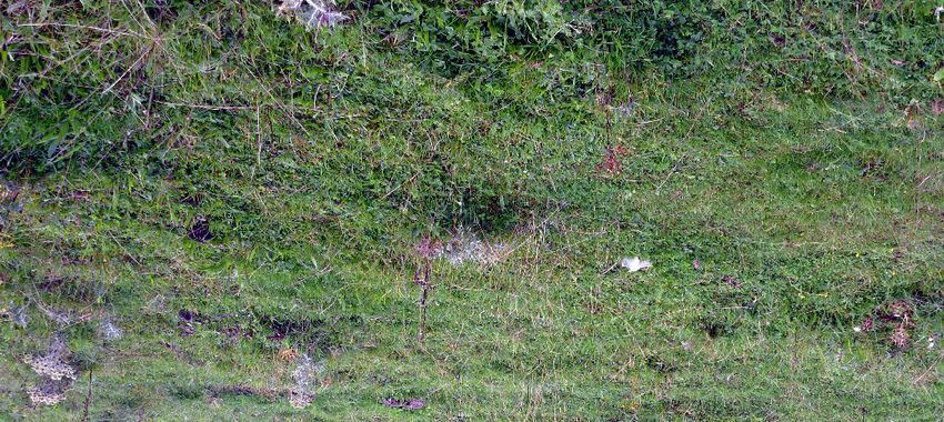
Remote Sens. 2018, 10, 1144                                                                         2 of 18

interesting characteristic to discriminate vegetation types by. Frequent monitoring of floodplain land
cover is necessary to capture the dynamics of floodplain vegetation and its related functions.
      Monitoring of floodplain land cover is commonly performed by making maps which are generally
obtained from remote sensing (RS) data. Detailed floodplain vegetation maps are commonly produced
by manually delineating and identifying vegetation objects using remote sensing data and visual
interpretation using a classification tree, e.g., for the Mississippi River [4], Murray-Darling Basin [5],
the Rhine Delta [6] and River Meuse [7]. However, low user’s accuracies have been reported for
production meadow, natural grasslands and herbaceous vegetation, whether they are obtained with
traditional airborne (user’s accuracy (UA) = 38–74%), high resolution spaceborne (57–75%) or Light
Detection And Ranging (LiDAR) remote sensing (57–73%) [8–11]. Even though vegetation height is
an important discriminator for floodplain vegetation types, this information is not available from
traditional airborne and spaceborne imagery and is difficult to obtain with an error less than 15 cm
with airborne LiDAR for low vegetation types [12]. Traditionally, the classification of floodplain
vegetation has mainly been performed with data sets collected at a single moment in time [13]. Several
studies have shown that the use of multitemporal data increases the classification accuracy, owing
to the different degrees of variation in the spectral characteristics of vegetation types through the
seasons [14–18]. These studies were carried out with satellite data, because of the relatively low costs
of obtaining imagery at a high frequency for large areas, compared with airborne imagery. However,
for semi-natural riverine landscapes, which are dominant in Europe, the low spatial resolution of the
spaceborne data limits the ability to differentiate between floodplain vegetation types. Furthermore,
while multitemporal data might improve the accuracy of floodplain vegetation maps, it is still unclear
how many and which moments during a year are optimal for the acquisition of monitoring data for
floodplain land-cover mapping. For example, Langley et. al. [19] found that time series of spectral data
do not always improve the grassland classification accuracy, due to similarities between vegetation
types at certain time steps or the effect of shadow during low sun angles in winter.
      In recent years, the increased availability of unmanned aerial vehicles (UAVs) has allowed low-cost
production of very high-resolution orthophotos and digital surface models (DSMs) [20]. These data
have high potential for floodplain vegetation monitoring, because they enable frequent production
of detailed greenness and vegetation height maps. Over time, height and greenness attributes may
improve the classification accuracy of floodplain vegetation patches, since these characteristics change
over the seasons in specific ways for different vegetation types [3]. An object-based classification of
riparian forests based on UAV imagery also indicated spectral and vertical structure variables as being
the most discriminating [21]. Time series of UAV images have mostly been used for elevation change
mapping studies, reporting vertical accuracies of 5–8 cm for bare surfaces [22–25]. To monitor the
crop height of barley, Bendig et al. [26] reported a vertical error of 0.25 m and for natural vegetation
UAV-derived DSMs can be used to estimate the vegetation height with an error of 0.17–0.33 m [3].
      A downside of a multitemporal dataset is the large number of variables available for classification,
of which only a small fraction is likely to contribute significantly. Consequently, a classification model
may tend to consider the less important variables (noise) as well for its predictions, which makes
it sensitive to overfitting. Model complexity and the number of available variables are important
components of a classification procedure to affect overfitting. A complex classification model, in
which a large number of variables are available for the prediction, may be more prone to overfitting,
because there is a higher possibility it will include noise variables in addition to high value variables.
Different levels of model complexity can be achieved by varying the number of variables the model
can include. Overfitting may also arise when using a large dataset with many variables. Further testing
is required to determine whether the number or type of variables used in the model can be optimized
in addition to the number of time steps considered.
      The manual identification of map units (objects) is a time-consuming method, which may be
bypassed by using a semi-automatic, object-based approach, in which a segmentation algorithm
groups the pixels into homogeneous objects. These objects are then classified based on the spectral
Remote Sens. 2018, 10, 1144 3 of 18
signal of the object, as well as the shape and context characteristics of the object. By using the signal of
the object instead of the pixel, the signal is amplified and, additionally, allows for the use of variation
within the object as an attribute [27]. Thus, combining multitemporal, UAV-derived, high-resolution
imagery with object-based classification techniques has the potential to offer a major step forward in
the automated mapping and monitoring of complex and dynamic floodplain vegetation in high detail.
The aims of this study were (1) to document floodplain land cover based on the classification
of multitemporal UAV-derived imagery with an object-based approach, focusing on low vegetation;
(2) to evaluate the effect of varying the number and timing of acquisition moments on the classification
accuracy of multitemporal input data versus single time step data; and (3) to quantify the effect of
different levels of complexity of the dataset and classification model on the classification accuracy.
2. Materials and Methods
2.1. Study Area
We performed our classification study on the embanked Breemwaard floodplain (Figure 1C).
The area of 116 ha is located on the Southern bank of the river Waal (Figure 1A), which is the
largest distributary of the river Rhine in the Netherlands. Typical vegetation in the Breemwaard
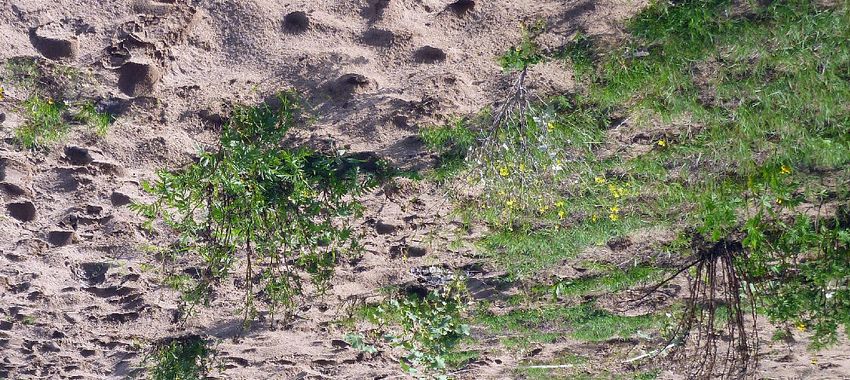
includes pioneer vegetation (e.g., scutch grass, tansy, narrow-leaved ragwort, and red fescue), natural
grassland (e.g., creeping cinquefoil, English ryegrass, red clover, and yarrow), production grassland
(e.g., English ryegrass and orchard grass), herbaceous vegetation (e.g., narrowleaf plantain, common
nettle, dewberry, water mint, creeping cinquefoil, and black mustard) reed and riparian woodland
(e.g., white willow, black poplar, and alder) (Figure 1B). Different management practices, such as
grazing and mowing, have resulted in a heterogenous distribution of these vegetation types. Along
the banks of the Waal bare sand, protection rock/rubble of groynes and pioneer vegetation are the
main surface cover. The four water bodies are the result of clay mining in the past. For a more detailed
description of the floodplain and its history, see Peters et al. [28].
4° E 5° E 6° E 7° E
A pioneer production grassland natural grassland B
´
53° N
North Sea
Breemwaard
52° N
herbaceous reed trees
m
Waal
Meuse Rhine
51°49'0"N 51° N
km
0 25 50 100
0 0.25
km
0.5
C
flow
direction
51°48'40"N
´
5°9'0"E 5°10'0"E
Legend
pioneer bare sand sealed road obtained from
production grassland trees
images
natural grassland herbaceous vegetation reed water rock/rubble
Figure 1. Breemwaard study area on the Southern bank of the river Waal. (A) Location in the Rhine
Delta; (B) Field impressions of typical vegetation in the study area; (C) Orthophoto of June with
classified reference polygons. Polygons marked with a dotted circle were obtained from the imagery
and the remaining polygons were obtained from the field.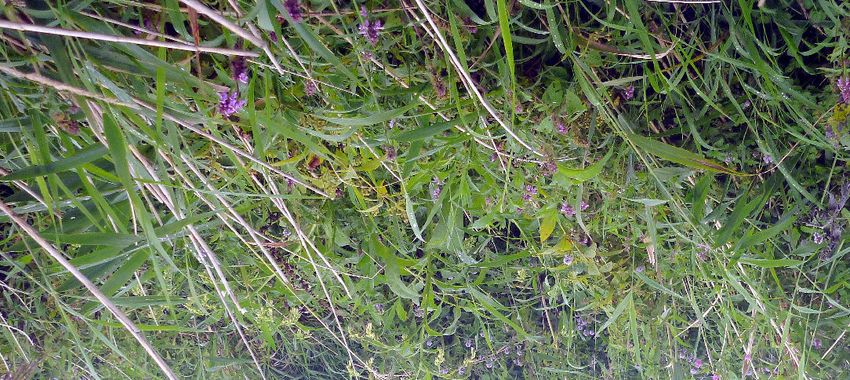
Remote Sens. 2018, 10, 1144                                                                          4 of 18

2.2. Data Set and Processing

2.2.1. Reference Data
      Reference data, representing homogeneous vegetation units, were collected in the field and
supplemented by digitized areas from orthophotos. Low floodplain vegetation (
Remote Sens. 2018, 10, 1144                                                                         5 of 18

                              Table 1. Total area of reference polygons per class.

                                           Class                Total Area (m2 )
                               1.     Pioneer vegetation               676
                               2.      Natural grassland              1986
                               3.    Production grassland              758
                               4.    Herbaceous vegetation            2975
                               5.            Reed                      621
                               6.          Bare sand                  1114
                               7.           Forest                    1662
                               8.            Water                    1211
                               9.         Sealed road                  198
                               10.       Rock/Rubble                   119

2.2.2. UAV Imagery Acquisition and Preprocessing
      Survey data were collected as described in Van Iersel et al. [3]. In brief, the UAV imagery was
collected at six moments during one growing season: February, April, June, September, and November
2015, and January 2016. The Swinglet CAM by Sensefly [29] was used as the platform for all flights,
except for June when we used a Sensefly eBee because of repair work on the Swinglet. A Canon IXUS
125 HS was used to acquire true colour (RGB) imagery and a modified Canon IXUS 125 HS for false
colour (CIR) imagery in two separate flights, because the UAV could only carry a single camera. The
surveys were conducted between 7 a.m. and 6 p.m., depending on the sunrise and sunset timing
which differed over the season, on days with low wind speeds and constant weather conditions. In
total, 38 white vinyl markers, supplemented by five street lanterns and road markings, were used
as ground control points (GCPs) for georeferencing. The obtained imagery was processed with
Surface-from-Motion (SfM) in Agisoft Professional [30] to obtain point cloud DSMs and orthophoto
mosaics of the study area [3]. Per survey, we obtained a true colour orthophoto (orthoRGB ), a true
colour DSM (DSMRGB ), a colour infrared orthophoto (orthoCIR ), and a colour infrared DSM (DSMCIR ),
resulting in 12 orthophotos and 12 DSMs. The orthophotos were raster formatted, whereas the DSMs
consisted of point clouds. Agisoft reported errors of less than 0.1 m in both the XY and Z directions for
its produced orthophotos and DSMs.

2.2.3. DSM and Orthophoto Processing
     The DSMs represented the elevation of the floodplain surface model above sea level, and not
the vegetation height. The height of each DSM point above the terrain surface (nDSM point ) was
calculated as the difference from a LIDAR bare earth model [31]. The terrain surface was based on the
LiDAR-based digital terrain model (DTM) of the Netherlands, which has a vertical accuracy of 5 cm for
bare earth. The nDSMs point were rasterized to a 25-cm grid (nDSMsraster ), to use them for segmentation
in the eCognition Developer software [32]. To match the orthophotos’ resolution, the point nDSM was
resampled into a 5-cm grid using nearest neighbour assignment. Large water areas were manually
masked in the nDSMsraster because of outliers in the dense point clouds due to matching errors in the
SfM method with the continuously changing water surface.
     The orthoCIR were used to calculate a vegetation index for each time step. The available spectral
channels of the CIR camera (blue, green and near infrared) did not allow the commonly used NDVI
based on red and near infrared to be calculated. Therefore, we used the blue channel instead of red and
calculated a ‘consumer-grade camera’ vegetation index (CGCVI) in accordance with Rasmussen et al.
and Van Iersel et al. [3,33]. A CGCVI layer was calculated for each time step, resulting in six additional
layers. After processing, three types of raster layers were obtained per time step: (1) single band
raster nDSMs; (2) three-band raster orthophotos; and (3) a single band raster CGCVI image. In total,
54 layers were available for multitemporal segmentation and classification: six nDSMsRGB,raster , six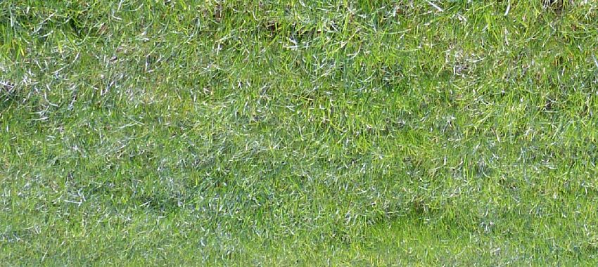
Remote Sens. 2018, 10, 1144                                                                                            6 of 18

nDSMsCIR,raster , six orthoRGB with three channels, six orthoCIR with three channels and six CGCVI
(Figure 3; input).

2.3. Methods
      To achieve the three research aims, we performed the analysis in three main steps (Figure 3).
First, we used the dataset of multitemporal UAV imagery and reference data to evaluate the
classification of floodplain land cover with an object-based approach. For the object-based approach,
segmentation was required, which is the process of grouping pixels of the image together into image
objects or segments [34], followed by classification of these segments during which, land-cover classes
are assigned to the objects. The raster layers were segmented and the obtained objects were classified
using a Random Forest (RF) classifier. Second, this process was repeated, leaving out the image data
from the time step that contributed the least to the overall classification accuracy until only the data
from one time step remained. In this way, we evaluated the effect of varying the number and timing
of acquisition moments of multitemporal input data versus single time step data. Third, to quantify
the effect of the different levels of complexity of the dataset and of the classification model on the
classification accuracy, the classification over a step-wise reduction of time steps was repeated with a
less complex RF and with a reduced input dataset.

                        Input                       Classification                        Timestep reduction

                         Six
                                                    Segmentation
                     time steps                  based on n*9 layers
                                                                                                      n=n-1
                        (n=6)

                       9 layers:

                        RedRGB                   Variable selection via
                                                  VarSelRF based on                       Drop TSleast from further
                       GreenRGB                    n*18 attributes                                analysis
                                                (mean & sd of 9 layers)
                        BlueRGB

                    Near InfraredCIR
                                                                                              Determine which time
                                               New segmentation based
                       GreenCIR                                                                steps add least value
                                               on VarSel-selected layers
                                                                                                      (TSleast)
                        BlueCIR

                       nDSMRGB
                                                                                              Perform n times RF
                        nDSMCIR                RF classification based on        If         classification based on
                                                n*18 object attributes          n >1      (n-1)*18 attributes: leave
                        CGCVI                                                              out each time step once

                                                             If n =1

                                                                          Application of RF
                                                                           classifier with
                                                                          highest accuracy
                                                                              to create
                                                                          land-cover map

                                                        Output

      Figure 3. Workflow of multitemporal segmentation, classification, and validation, resulting in accuracy
      by decreasing the number of time steps. The subscript RGB indicates a true colour layer and CIR
      indicates a false colour. Random Forest (RF) and varSelRF are classification models in R.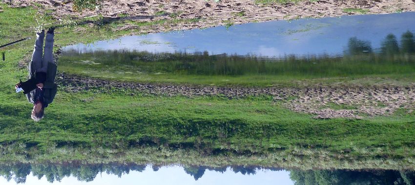
Remote Sens. 2018, 10, 1144                                                                           7 of 18

2.3.1. Object-Based Multitemporal Classification and Validation
     To perform an object-based image classification, the 54 raster layers were first segmented.
The obtained segments were assigned 108 spectral and height attributes, which were calculated
from the 54 raster layers (i.e., 54 mean & 54 standard deviation (SD)). Second, we performed an
RF classification to select the most discerning attributes of the objects. In a third step, a new image
segmentation was carried out, now using the layers on which these most important attributes were
based and independent of earlier obtained segments. Fourth, this second segmentation was again
classified with an RF to check the classification accuracy and to determine the attributes from which
time step contributed least to the classification accuracy. This processing loop was repeated five times,
each time leaving out the time step that contributed least to the classification (Figure 3).

Segmentation
      Many object-based classifications have shown superior results over pixel-based landscape
classification [34]. In vegetation classification, the within-area statistics of the pixels making up
the object are an interesting feature, because some vegetation objects, such as a patch of herbaceous
vegetation, are expected to show a relatively large internal variation in colour and height compared
with smoother grassland objects. For this reason, the layers were segmented into objects before
classification, using eCognition Developer [32]. To compare our vegetation objects from the imagery
with the field reference data, an object size less than the field-plot size was necessary, which was
achieved with a scale parameter setting of 60 for all 54 layers. The shape and compactness were both
set to 0.1. An object was selected for the training or validation of the classification if it overlapped
at least 50% with a reference polygon. If it overlapped with more than one polygon, it was assigned
the class with which it shared at least 50% of its surface area. The attributes per object were (1) class;
(2) the X and Y coordinates of the object centre; (3) the mean value of each layer; and (4) the standard
deviation of each layer.

Variable Selection and Second Segmentation
      All reference objects obtained from the segmentation were divided into two sets of equal size by
splitting them alternately per class based on their X-coordinate into a training and validation dataset.
This was done to ensure an equal number of objects per class in both the training and validation sets
and to make sure both sets represented the variation in the entire study area. For classes with more than
1000 objects, a random sample of 1000 objects was taken first, which was then divided into the training
and validation sets, as described above. All classes except sealed road and rock/rubble had more than
1000 objects. The function varSelRF in R [35] was used to select the most discerning attributes of the
multitemporal data set. During this selection step, all attributes were included, thus variables of all
time steps could be selected. VarSelRF iterates over multiple RF classifications, dropping variables
until the out-of-the-bag-error (OOB) becomes larger than the initial OOB error until only the relevant
variables remain. Although the varSelRF is also a classifier, here, it was only used for attribute selection.
A new segmentation was then performed in eCognition to obtain segments based on only the layers of
these selected attributes. The objects of the varSelRF segmentation were exported as described in the
previous section.

Classification
     The varSelRF-based objects were again sampled up to 1000 objects and alternately split into
training and validation datasets based on their X-coordinate. An RF classifier was built in R based on
these samples for each class from the training set and using all 108 attributes. The RF classifier was
built with 10,000 trees, and the maximum number of end nodes (maxnodes) was set to 25 to prevent
overfitting (RFmaxn=25 ). In data sets with a large number of variables, it is likely that only a small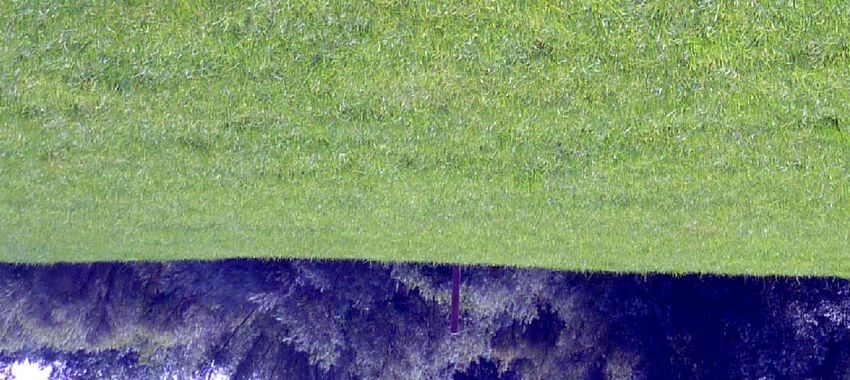
Remote Sens. 2018, 10, 1144                                                                         8 of 18

fraction of these contribute significantly to a high accuracy level. An unrestrained classification model
may tend to consider noise variables as well for its predictions, which could lead to overfitting.

Validation
     The classification accuracy of the RF was determined using the independent validation set and
was reported as the overall classification accuracy (OA) and Kappa statistic (κ). OA is the percentage
of true positives in all evaluated objects and (κ) corrects the OA for the possibility of an agreement
occurring by chance. The OA and κ were calculated from the confusion matrix, which accounted
for the area of the objects in order to correct for object size. To check for overfitting of the RF model,
an additional validation was performed with the training dataset, resulting in an OAtrain and κtrain .
For the difference between OAval and OAtrain ≤ 0.01 percent point (pp), overfitting was assumed
negligible. Moreover, the user’s accuracy was used to inspect the performance of individual classes
from the point of view of a map user, as it shows how often the class on the map will actually be
present on the ground. The producer’s accuracy indicates how often real objects of this class on the
ground correctly show on the classified map.

2.3.2. Classification Accuracy with Step-Wise Decrease in the Number of Time Steps
     Since the costs for monitoring are directly related to the number of surveys carried out (i.e., time
steps), the relation between the number of monitoring time steps per year and the resulting OA is of
high relevance. To determine which moments are essential, the time step contributing the least to the
OA (TSleast ) was dropped repeatedly from the segmentation and classification, until only one time step
remained (Figure 3). To determine the TSleast of the total of six time steps, the RF was performed six
times, each time leaving out either February, April, June, September, November, or January. TSleast was
selected from the RF loop with the least decrease or even increase in OA compared to the condition
where all time steps were included and the layers and derived attributes of TSleast were excluded from
further analyses.
     The next step was to find the TSleast of the remaining time steps with the same method, for which
we subsequently performed a new segmentation, variable selection, a second segmentation with the
optimal layers from five time steps and five times the RF including only four time steps. These steps
were repeated until only a single time step remained (Figure 3). To guarantee similar object sizes
over the entire work flow, the scale parameter was adjusted in each segmentation to maintain
5 × 10⁶ ± 10% segments for the whole study area.

2.3.3. Varying Complexity of the Classification Model and the Data Set
      Two additional analyses were performed with the six segmentations that included layers of one
to six time steps. This means that the first three blocks in the “Classification” of Figure 3 were skipped
to reduce calculation time, but the rest of the method was repeated. First, maxnodes was set to default
for the best obtainable RF model (RFde f ault ) for the Breemwaard dataset. With maxnodes set as inactive,
the RF can build each tree to its maximum depth [36]. In this case, each tree may consider noise
variables as well for its predictions, which increases the risk of overfitting. Second, the RFs were built
using only the spectral attributes (RFspectral ) and excluding the nDSM attributes. In this way, the added
value of multitemporal data with and without elevation data could be determined. Note that the
segments used for this additional analysis were obtained by segmenting both the spectral and nDSM
layers. Maxnodes was kept at 25.
      The RF classifier with the highest OA was applied to the corresponding layers to classify the
entire study area. The result of this classification was visualized by mapping the classified objects
of the entire study area, and this thematic map was compared to the orthophoto of September by
visual inspection.
Remote Sens. 2018, 10, 1144                                                                                       9 of 18

3. Results

3.1. Object-Based Multitemporal Classification
     From the available 54 layers (nine layers x six time steps), for the first multitemporal segmentation,
the varSelRF function selected 23 out of 108 attributes, including (1) only mean attributes; (2) all mean
nDSM attributes; and (3) all mean CGCVI attributes. No SD attributes were selected by varSelRF.
The second segmentation, performed with only the layers of the varSelRF-selected attributes, resulted
in an OA of 0.939 and a κ of 0.926 (Table 2).

      Table 2. Classification accuracy with step-wise decrease in the number of time steps. The * indicates
      the time step which adds the least value. This time step is the group of 18 attributes collected for this
      specific time step and is not used in further analyses. OA is the overall classification accuracy and κ is
      the Kappa coefficient. The subscript val indicates that validation is based on a validation data set and
      train is based on a training data set. Bold OAval show the accuracy of the RF with the same time steps
      used for the segmentation, which are plotted in Figure 4, labelled as ‘maxnodes-25’.

       Time Steps Included      Time Step Excluded       OAval     κval   OAtrain    κtrain   OAtrain    κtrain
       in Segmentation          from Classification      (%)       (%)    (%)        (%)      -OAval     -κval
                                          -               93.9     92.6     94.5     93.3     0.60       0.78
                                        FEB *             94.1     92.8     94.6     93.5     0.51       0.67
               n=6                      APR               93.8     92.5     94.4     93.3     0.63       0.82
           FEB APR JUN                  JUN               93.2     91.7     94.1     92.9     0.92       1.16
           SEP NOV JAN                   SEP              92.9     91.4     94.0     92.7     1.03       1.30
                                        NOV               93.8     92.5     93.2     94.4     −0.58      1.91
                                        JAN               93.8     92.4     92.4     93.2     −1.36      0.83
                                           -              94.1     92.7     94.1     92.8     0.01      0.04
                                         APR              93.6     92.1     93.7     92.3     0.10      0.14
              n=5
                                         JUN              93.0     91.4     93.2     91.6     0.15      0.20
           APR JUN SEP
                                         SEP              93.3     91.8     93.5     92.0     0.20      0.27
            NOV JAN
                                        NOV               93.8     92.4     93.8     92.4     −0.04     −0.03
                                        JAN *             94.1     92.7     94.1     92.7     −0.05     −0.05
                                          -               94.1     92.7     95.0     93.9      0.93      1.24
                                        APR               94.0     92.5     94.5     93.3      0.53      0.76
              n=4
                                        JUN               92.7     91.0     93.7     92.3      0.98      1.33
        APR JUN SEP NOV
                                        SEP               93.4     91.9     94.4     93.2      0.98      1.31
                                       NOV *              94.0     92.6     95.1     94.0      1.04      1.37
                                          -               94.4     93.2     94.4     93.2     −0.02     0.04
              n=3                       APR *             94.5     93.3     94.5     93.3     −0.06     −0.02
           APR JUN SEP                  JUN               91.2     89.2     91.1     89.2     −0.12     −0.07
                                         SEP              92.8     91.2     92.9     91.4     0.18      0.28
                                          -               94.6     93.4     94.6     93.3      0.00     −0.10
                n=2
                                        JUN               88.3     85.6     89.6     87.0      1.29     1.40
              JUN SEP
                                        SEP *             92.1     90.3     92.5     90.7      0.43     0.39
                n=1
                                           -              91.6     89.6     91.3     89.2     −0.29     −0.41
                JUN

3.2. Classification Accuracy with Step-Wise Decrease in the Number of Time Steps
     Table 2 shows the classification accuracies after subsequently leaving out a time step with
maxnodes set to 25. For each of the six segmentations, the classification accuracies are given for
every possible n−1 combination of the remaining time steps. The number of time steps included in the
segmentation decreases in each row with TSleast , which was based on the highest OAval obtained after
the time step was omitted (marked by the *). For example, for n = 6, the OAval even increased from
93.9% to 94.1% when February (FEB) was omitted. Moreover, OAval continued to increase until n = 2,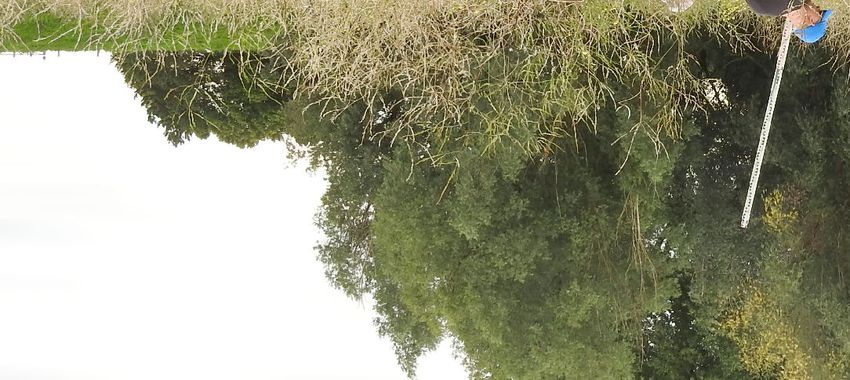
Remote Sens. 2018, 10, 1144                                                                                10 of 18

even though the differences in OAval were minimal (Figure 4, maxnodes-25). The most important
time step is June, because it was the last remaining time step and thus, was never selected as the least
contributing. In increasing order of importance, February, January, April, November, and September
were shown to be TSleast .
      All classifications with the RFmaxn=25 resulted in high OAval and κval , both exceeding 90%. The OA
and κ were higher for the multitemporal sets than those obtained for the remaining single time step in
June (Figure 4). The differences in OA and κ were remarkably small among the different multitemporal
sets. The highest accuracy was achieved using the June and September datasets; the OAval was 94.6%,
compared with 91.6% for June only. This means that adding September’s data to the classification based
solely on June increased the classification by 3 percent point (pp), which thus decreased the initial
error of 8.4% by about one-third. Overfitting was not an issue in any classification, as OAtrain -OAval
was equal to or less than 1.36 pp (Table 2). User’s accuracies exceeded 85% for all classes except for
natural grassland (60–73%) for 1–6 time steps (Table S1). This may be explained by its high within-class
variability and confusion between the pioneer and herbaceous vegetation classes, due to structural
and spectral similarity.

3.3. Varying Complexity of the Classification Model and Data Set
     The RFde f ault resulted in significantly higher OAs compared to the less complex RFmaxn=25
(p = 0.00001) (Figure 4). We found the highest accuracy when including all six time steps: the OAval
was 99.3%, compared to 96.9% for June only. This is an increase in accuracy of 2.4 pp, which equals
a 76% decrease in classification error. With RFde f ault , the OA decreased much more gradually when
eliminating time steps, compared with the sudden decrease in OA and κ at one time step obtained with
RFmaxn=25 . User’s accuracies exceeded 75% for all classes, even when using one time step, and were
larger than 90% for three time steps or more. Overfitting was only a minor issue with RFde f ault , as
OAtrain -OAval stayed below 3 pp. Validation with the training set resulted in an accuracy of 100%.

                                      100%
                                      98%
                                      96%
                                      94%
                                      92%
                              OAval

                                      90%
                                      88%
                                      86%           maxnodes-default
                                      84%           maxnodes-25
                                      82%           only spectral
                                      80%

      Figure 4. Accuracy of the RF classification by decreasing number of time steps. OAval is the
      classification accuracy based on validation with an independent data set. For only spectral attributes,
      maxnodes was 25.
Remote Sens. 2018, 10, 1144 11 of 18
When the nDSM-related attributes were excluded from the RF classification, the OA was
significantly lower (p < 0.01) compared with RFmaxn=25 (Figure 4). The OA increased from 86%
to 92% by using three or more time steps. However, reed and herbaceous vegetation still had user’s
accuracies of 51–68%. Error matrices of n = 1 and n = 6 for the three levels of complexity can be found
in the Supplementary Information (Table S2).
3.4. Classified Land-Cover Map
The natural vegetation types only have small differences in their spectral and structural
characteristics, but they were well discriminated by the RF (Table 3). Pioneer vegetation is sometimes
confused with bare sand, which is understandable as this sparse vegetation does not fully cover
the bare sand. Overall, the classification with RFde f ault matched the vegetation patterns that were
observed on the orthophoto at the end of the growing season (September) (Figure 5A). The production
grassland area in the east was well delineated. The detailed alternating patterns of natural grassland
and herbaceous vegetation were also excellently mapped. For example, the stripy pattern in the
centre of the floodplain is caused by small terrain height differences of approximately 0.4 m, which
results in different vegetation types in the lower (grassland) and higher (herbaceous) sections
(Figures 4C and 5B). These terrain height differences are man-made remnants of old forestry methods
from the 19th and 20th centuries, so-called rabatten. Along the banks of the water bodies, wet pioneer
vegetation or wet bare sand is sometimes classified as rock or sealed road, which is understandable
due to its low reflectance and irregular surface that are similar to the rock/rubble class (Figure 5A).
5°8'30"E 5°9'0"E 5°9'30"E 5°10'0"E 5°10'30"E
Legend A
bare sand sealed road
51°49'0"N
pioneer
natural grassland trees rock/rubble
production grassland water
herbaceous vegetation
reed
C'
51°48'45"N
0 0.1250.25 0.5 0.75 1
km
´
B C
51°48'49"N
51°48'49"N
51°48'47"N
51°48'47"N
0 12.525 50 75 100 0 12.525 50 75 100
m m
5°9'25"E 5°9'30"E 5°9'25"E 5°9'30"E
Figure 5. Classified land-cover map of the Breemwaard floodplain with data from the best performing
RF, which used data from all time steps and maxnodes set to default. (A) Overview of the classified
study area. (B) Orthophoto of September of zoomed in area C’ and (C) zoomed in area of classified
grassland and herbaceous vegetation.Remote Sens. 2018, 10, 1144 12 of 18
Table 3. Confusion matrix of the RF classification based on all six time steps and with maxnodes of the RF set to default, expressed in numbers of pixels.
Reference
Pioneer Vegetation Sealed Road Rock/Rubble Natural Grassland Prod. Grassland Herb. Vegetation Reed Bare Sand Forest Water User’s Accuracy
Pioneer Vegetation 57,317 0 0 0 0 0 0 765 0 0 99%
Sealed road 0 38,362 0 0 0 0 0 0 0 0 100%
Rock/Rubble 23 0 23,152 0 0 0 0 0 0 0 100%
Natural grassland 0 0 0 72,422 0 2210 0 0 0 0 97%
Prediction Production grassland 0 0 0 0 110,501 0 0 0 0 0 100%
Herbaceous vegetation 60 0 0 1993 0 40,616 0 0 0 0 95%
Reed 0 0 0 0 0 0 24,759 0 0 0 100%
Bare sand 378 0 0 0 0 0 0 117,974 0 0 100%
Forest 0 0 0 0 0 0 0 0 22,953 0 100%
Water 0 0 0 0 0 0 0 0 0 245,643 100%
Producer’s accuracy 99% 100% 100% 97% 100% 95% 100% 99% 100% 100%Remote Sens. 2018, 10, 1144 13 of 18
4. Discussion
This is the first study to use UAV multi-seasonal data for object-based classification of natural
non-woody vegetation at a high spatial resolution, according to the authors’ knowledge. High overall
accuracies of more than 90% were found, even with a single time step. The high classification accuracies
were caused by the additional attributes on vegetation height compared with traditional airborne
imagery which reports lower OAs of 75–77% [9–11], as well as the powerful RF classifier.
4.1. Object-Based Multitemporal Classification
The varSelRF function showed that only the object means of layers were relevant attributes,
whereas SD attributes were unimportant. Although the variation within the objects did not show up
as an important attribute, the object-based approach is still recommended because of noise reduction.
Calculating the mean or another measure of central tendency for an object reduces the effect of
extreme pixel values and decreases noise [37]. Hence, object-based classification decreases the spectral
confusion of classes.
Weil et al. [38] were able to classify herbaceous patches within in a Mediterranean woody
vegetation with a user’s accuracy of 97.1% and an OA of 85% with only spectral UAV data. However,
their “herbaceous patches” class included all low vegetation, whilst all other classes were specific tree
species; in our study, we differentiated several low vegetation classes and still obtained high OAs.
This detailed classification of low vegetation types is required to map hydraulic roughness in river
flood modelling [39]. In addition, it is the level of detail at which the habitat characteristics of small
floodplain fauna such as butterflies need to be monitored [40]. Other studies classifying similar natural
vegetation with multitemporal satellite data yielded lower OAs of 80–90%, but also produced maps
covering much larger areas [14,16]. The high classification accuracies found with multitemporal UAV
imagery are owing to (1) the high resolution combined with an object-based approach [41]; (2) the
addition of vegetation height data, which is of major importance when discriminating between classes
like grassland, shrub, and herbaceous vegetation [3,9]; and (3) the use of an RF classifier which was
also proven to be the most powerful by Weil et al. [38] using multitemporal data.
4.2. Required Number of Time Steps
OA and κ are up to 3 pp higher for the multitemporal sets than those of the single time step for
June, produced with RFde f ault , RFmaxn=25 and RFspectral . Interestingly, for the less complex RFmaxn=25 ,
the differences in OA and κ were minimal between the different multitemporal sets. Weil et al. [38]
also found no prominent improvements in OA in their RF classification of woody vegetation after the
first three optimal time steps. Most likely, the RF did not produce a sufficiently large majority of trees
containing the important variables, due to the pre-set limitation on the number of end nodes. This may
be explained by the small difference in the added value to the classification accuracy between the
included variables and the high number of variables involved in the classification with more than two
time steps. As a result, classification using a larger number of attributes (in this case, based on more
time steps) might not necessarily result in higher OA. In this study, this mostly affected the user’s
accuracies of classes with a high internal variability, such as natural grassland, because the restricted
trees in RFmaxn=25 do not capture this variability. When only using the June data, important variables
were clearly missing in the forest, resulting in a much lower OAval .
The highest OA was found when combining June and September, which may be explained
by the fact that June has the moment of maximum photosynthetic activity, and hence, the highest
CGCVI, while in September, most vegetation is at its maximum height. Hence, spectral and structural
differences between vegetation types are most pronounced in these months, while data from other
months become redundant, add noise, and may increase confusion between classes. These findings are
similar to what Michez et al. [21] concluded from their multitemporal study classifying riparian forestRemote Sens. 2018, 10, 1144 14 of 18
species. They found that the late vegetation season was the most appropriate time window to perform
UAV surveys, because phenological differences between riparian forest species are the most enhanced.
4.3. Varying Complexity of the Classification Model and of the Data Set
The RFde f ault had overall higher OAs than RFmaxn=25 , because the trees were built to their full
extent. It was possible for each training object to have its own end node in these fully grown trees.
However, this also increased the risk of using noisy variables to build the tree, potentially causing
overfitting on the training data. Therefore, we built a large number of trees (i.e., 10,000) to correct for
overfitting [36], and the differences between OAval and OAtrain of 0.03 or less show that overfitting
was indeed minimal [42].
Multitemporal data is also of high value for classifications based only on spectral UAV data.
The OA obtained using spectral information increased from 86% when based on a single observation
moment to 92% when data acquired during three or more time steps were used. Even with
multitemporal data, user’s accuracies obtained for reed and herbaceous vegetation were low
(Supplementary Information, Table S1), because without height information, these classes are easily
confused with each other or with spectrally similar classes such as natural grassland. Note that the
objects used in RFspectral were obtained from segmentation of both nDSM and spectral raster layers.
The less complex RFmaxn=25 classifier is sensitive to the number of variables, as using data
from more than two time steps did not improve, and even decreased, the OA (Figure 4). This
counterintuitive result is due to the large number of variables, of which many are correlated or not
discriminative between classes, which hampers identification of the important variables in the RF
procedure. This effect is negligible when a smaller total number of variables per time step is available,
as was the case with only spectral attributes of the objects. Moreover, OA improved significantly
when using the default tree depth (RFde f ault ) instead of a limited depth (RFmaxn=25 ), because the larger
number of tree nodes led to more frequent selection of the important variables, hence leading to a
better overall RF classification performance.
4.4. Training and Validation Sets
The RF performance is also sensitive to the number of classes and the number of objects per
class. In a few experimental runs with more classes, for example, quite similar types of herbaceous
vegetation, the RF developed a preference towards one of these classes and misclassified the other
class, instead of confusing them equally. In the experiment, the class with the highest internal variation
was predicted the least, unless its number of objects was increased to better capture the within-class
variation by the trees of the RF. Moreover, the RF was susceptible to the resemblance of the training
and validation sets. In our study the validation and training objects were obtained from the same
reference polygons. Switching the training and validation sets resulted in OAs of the same order of
magnitude (Figure S3), again with June and September being the most important time steps (Table S2) .
Surprisingly, if the polygons were first split into either training or validation, the resulting RF would
sometimes fit the validation data better than the training data. On the other hand, the structured
X-coordinate-based splitting of the reference objects into training and validation sets resulted in high
spatial correlation between the sets. Random sampling of the reference objects also resulted in OAs of
the same order of magnitude (Figure S3) with June and September being the most important time steps
(Table S3). Most importantly, the improvement in OA with multitemporal input data versus single
time step input data was still clear with different sampling methods for the training and validation
sets (Figure S3).
4.5. Floodplain Vegetation Map
The highest OA of floodplain vegetation was obtained with UAV imagery of all six monitoring
moments and an RF with default settings that built 10,000 trees. The alternations in grassland and
herbaceous vegetation were mapped in very high detail. We observed many different patterns in theseRemote Sens. 2018, 10, 1144 15 of 18
vegetation types, resulting from topographical or substrate differences, or grazing by cows and horses.
Mapping errors still occurred between non-vegetation classes, which gained little benefit from using
multitemporal data because they are relatively stable over time. These classes may benefit from a
different sensor that is able to detect reflectance in the short-wave spectrum (1700–2300 nm) where the
spectral differences between these materials are more pronounced [43]. Nevertheless, to document
natural floodplain vegetation, the spectral characteristics used in our study were satisfactory, as we
found user’s accuracies of 95% and higher.
The improvement in land-cover-map accuracy with our method compared with other floodplain
land-cover-classification studies [8–11] has important consequences for applications in hydrodynamic
predictions and biodiversity estimations for floodplains. Straatsma et al. [44] predicted a reduction
of 50% in the uncertainty of discharge distribution over the bifurcation points of rivers with an
increase in the OA of floodplain land cover from 69% to 95%. We showed that this level of accuracy
is now achievable for natural floodplain vegetation with multitemporal UAV data. More detailed
maps allow for more detailed management of floodplains, for example, by allowing more complex
spatial configurations of vegetation types, while maintaining overall safe conditions during high river
discharge. A higher diversity in vegetation structure may be relevant as it is typical of the habitat
of floodplain fauna. However, quantitative ecological knowledge on habitat characteristics, such as
the spatial configurations of vegetation types, is species-specific. Some studies on small floodplain
mammals have described, in detail, the necessary sizes and shapes of vegetation or other land-cover
types [45,46], but these are rare. Habitat suitability is often based on expert knowledge which is more
difficult to find and standardize for use in floodplain management.
4.6. Practical Considerations
For practical application, UAVs allow high-resolution and frequent monitoring areas of a few
square kilometres, since image acquisition takes three days for an area of roughly 100 ha (1 day of
flying and 2 days for GCP collection). For data collection over much larger areas, this method becomes
costly. For example, a UAV survey of the entire Dutch Rhine delta would take 370 km2 × 3 days
= 1110 days, which would require 50 simultaneously working survey teams of 2 people to collect
the data within a month (22 working days) and would cost approximately one million euros. For a
cost-benefit analysis, it would be interesting to compare these costs to those of traditional airborne
imagery acquisition from a plane or helicopter of the same region with a similar resolution of 5 cm and
sufficient image overlap of 60% or more.
The above calculation excludes the costs for the LiDAR DTM which was used for normalization
of the UAV DSMs. However, this can be obtained once every few years depending on the floodplain
topography dynamics. Another possibility might be normalization of the DSMs with a sparsely
vegetated winter DSM, which would be fine for the low, non-woody vegetation [3], but the nDSMs
would become inaccurate for more woody vegetation as they maintain their height in winter and block
the view of the terrain for the UAV.
5. Conclusions
We collected a large multitemporal data set with high resolution vegetation height and spectral
information, which resulted in the availability of 108 variables for the object-oriented classification of
floodplain land cover. Using data from six UAV surveys over a growing season and a Random Forest
classifier (RF), we obtained overall classification accuracies of up to 99.3% and user’s accuracies of at
least 95%, even for similar classes, such as natural grassland and herbaceous vegetation. This high
accuracy of floodplain land-cover maps has important implications for floodplain management, as it
will improve hydrodynamic predictions and biodiversity estimations.
With the RF, we were also able to filter the many variables of the multitemporal dataset in terms
of importance for the monitoring of floodplain land cover. With default RF settings, the use of two or
more time steps compared with a single time step increased the overall classification accuracy fromRemote Sens. 2018, 10, 1144 16 of 18
96.9% up to 99.3%. The most important time steps were June and September, which is when most
floodplain vegetation reaches its maximum values for, respectively, greenness and vegetation height.
Additional testing with varying RF complexity and a smaller data set showed that overfitting was not
a major problem, because the difference between validation with the training set and independent
validation set was less than 3 percent points.
Our method is a practical solution for monitoring areas of a few km2 . The same method can be
used for large-scale monitoring of floodplains, but with data from airborne platforms covering larger
extents. Our study can be used to improve the survey setup and planning with these platforms.
Supplementary Materials: The following are available online at http://www.mdpi.com/2072-4292/10/7/1144/s1,
Figure S1. The nine field plots containing a mixture of two vegetation types, Figure S2. Field impressions of
the vegetation types in the Breemwaard study area, Figure S3. Accuracy of the RF classification by decreasing
number of time steps for different sampling of the training and validation sets from the reference data, Table S1.
Error matrices of classifications with 1) RFmaxn=25 and RFde f ault with structural and spectral data and RFmaxn=25
with only spectral data for segmentations with six (n = 6) and one (n = 1) time steps, Table S2: Classification
accuracy with step-wise decrease in number of time steps with reversed training and validation set in the
RandomForest classification, Table S3: Classification accuracy with step-wise decrease in number of time steps
with random sampling of training and validation set per class.
Author Contributions: Conceptualization, W.v.I., M.S., H.M. and E.A.; Data curation, W.v.I.; Formal analysis,
W.v.I.; Funding acquisition, H.M.; Investigation, W.v.I.; Methodology, W.v.I. and E.A.; Supervision, M.S., H.M. and
E.A.; Validation, W.v.I.; Visualization, W.v.I.; Writing—original draft, W.v.I.; Writing—review & editing, W.v.I.,
M.S., H.M. and E.A.
Funding: This research is part of the research programme RiverCare, supported by the Dutch Technology
Foundation TTW (formerly STW), which is part of the Netherlands Organization for Scientific Research
(NWO), and which is partly funded by the Ministry of Economic Affairs under grant number P12–14
(Perspective Programme).
Acknowledgments: The authors would like to thank the State Forestry for its permission to fly with the UAV in
the Breemwaard. All volunteers are greatly acknowledged for their assistance during the field surveys.
Conflicts of Interest: The authors declare no conflict of interest.
References
1. Tockner, K.; Pusch, M.; Borchardt, D.; Lorang, M.S. Multiple stressors in coupled river-floodplain ecosystems.
Freshw. Biol. 2010, 55, 135–151. [CrossRef]
2. Schindler, S.; Sebesvari, Z.; Damm, C.; Euller, K.; Mauerhofer, V.; Schneidergruber, A.; Biró, M.; Essl, F.;
Kanka, R.; Lauwaars, S.G.; et al. Multifunctionality of floodplain landscapes: Relating management options
to ecosystem services. Landsc. Ecol. 2014, 29, 229–244. [CrossRef]
3. Van Iersel, W.K.; Straatsma, M.W.; Addink, E.A.; Middelkoop, H. ISPRS Journal of Photogrammetry and
Remote Sensing Monitoring height and greenness of non-woody floodplain vegetation with UAV time series.
ISPRS J. Photogramm. Remote Sens. 2018, 141, 112–123. [CrossRef]
4. Dieck, J.; Ruhser, J.; Hoy, E.; Robinson, L. General Classification Handbook for Floodplain Vegetation in Large River
Systems; Technical Report Book 2; U.S. Geological Survey Techniques and Methods: Reston, VA, USA, 2015.
5. Eco Logical Australia. Vegetation of the Barwon-Darling and Condamine-Balonne Floodplain Systems of New South
Wales Mapping and Survey of Plant Community Types; Technical Report; Eco Logical Australia: Sutherland,
Australia, 2015.
6. Houkes, G. Toelichting Ecotopenkartering Rijntakken-Oost 2005; Technical Report; Rijkswaterstaat,
Data-ICT-Dienst: Delft, The Netherlands, 2008.
7. Daphnia Ecologisch Advies. Ecotopenkartering Maas 2004; Biologische Monitoring Zoete Rijkswateren;
Technical Report; Rijkswaterstaat: Brussels, Belgium, 2007.
8. Van der Sande, C.J.; de Jong, S.M.; de Roo, A.P. A segmentation and classification approach of IKONOS-2
imagery for land cover mapping to assist flood risk and flood damage assessment. Int. J. Appl. Earth
Obs. Geoinf. 2003, 4, 217–229. [CrossRef]
9. Geerling, G.W.; Labrador-Garcia, M.; Clevers, J.G.P.W.; Ragas, A.M.J.; Smits, A.J.M. Classification of
floodplain vegetation by data fusion of spectral (CASI) and LiDAR data. Int. J. Remote Sens. 2007,
28, 4263–4284. [CrossRef]Remote Sens. 2018, 10, 1144 17 of 18
10. Straatsma, M.W.; Baptist, M.J. Floodplain roughness parameterization using airborne laser scanning and
spectral remote sensing. Remote Sens. Environ. 2008, 112, 1062–1080. [CrossRef]
11. Knotters, M.; Brus, D.J. Purposive versus random sampling for map validation: A case study on ecotope
maps of floodplains in the Netherlands. Ecohydrology 2013, 6, 425–434. [CrossRef]
12. Straatsma, M.W.; Middelkoop, H. Extracting structural characteristics of herbaceous floodplain vegetation
under leaf-off conditions using airborne laser scanner data. Int. J. Remote Sens. 2007, 28, 2447–2467.
[CrossRef]
13. Xie, Y.; Sha, Z.; Yu, M. Remote sensing imagery in vegetation mapping: a review. J. Plant Ecol. 2008, 1, 9–23.
[CrossRef]
14. Wang, C.; Hunt, E.R.; Zhang, L.; Guo, H. Phenology-assisted classification of C3 and C4 grasses in the U.S.
Great Plains and their climate dependency with MODIS time series. Remote Sens. Environ. 2013, 138, 90–101.
[CrossRef]
15. Son, N.T.; Chen, C.F.; Chen, C.R.; Duc, H.N.; Chang, L.Y. A phenology-based classification of time-series
MODIS data for rice crop monitoring in Mekong Delta, Vietnam. Remote Sens. 2013, 6, 135–156. [CrossRef]
16. Simonetti, D.; Simonetti, E.; Szantoi, Z.; Lupi, A.; Eva, H.D. First Results from the Phenology-Based Synthesis
Classifier Using Landsat 8 Imagery. IEEE Geosci. Remote Sens. Lett. 2015, 12, 1496–1500. [CrossRef]
17. Yan, E.; Wang, G.; Lin, H.; Xia, C.; Sun, H. Phenology-based classification of vegetation cover types in
Northeast China using MODIS NDVI and EVI time series. Int. J. Remote Sens. 2015, 36, 489–512. [CrossRef]
18. Senf, C.; Leitão, P.J.; Pflugmacher, D.; van der Linden, S.; Hostert, P. Mapping land cover in complex
Mediterranean landscapes using Landsat: Improved classification accuracies from integrating multi-seasonal
and synthetic imagery. Remote Sens. Environ. 2015, 156, 527–536. [CrossRef]
19. Langley, S.K.; Cheshire, H.M.; Humes, K.S. A comparison of single date and multitemporal satellite image
classifications in a semi-arid grassland. J. Arid Environ. 2001, 49, 401–411. [CrossRef]
20. Nex, F.; Remondino, F. UAV for 3D mapping applications: A review. Appl. Geomatics 2014, 6, 1–15. [CrossRef]
21. Michez, A.; Piégay, H.; Lisein, J.; Claessens, H.; Lejeune, P. Classification of riparian forest species and health
condition using multi-temporal and hyperspatial imagery from unmanned aerial system. Environ. Monit.
Assess. 2016, 188. [CrossRef] [PubMed]
22. Tanteri, L.; Rossi, G.; Tofan, V.; Vannocci, P.; Moretti, S.; Casagli, N. Multitemporal UAV Survey for Mass
Movement Detection and Monitoring; Work World Landslide Forum: Ljubljana, Slovenia, 2017; pp. 153–161.
23. Esposito, G.; Mastrorocco, G.; Salvini, R.; Oliveti, M.; Starita, P. Application of UAV photogrammetry for
the multi-temporal estimation of surface extent and volumetric excavation in the Sa Pigada Bianca open-pit
mine, Sardinia, Italy. Environ. Earth Sci. 2017, 76, 1–16. [CrossRef]
24. Cook, K.L. An evaluation of the effectiveness of low-cost UAVs and structure from motion for geomorphic
change detection. Geomorphology 2017, 278, 195–208. [CrossRef]
25. Lucieer, A.; de Jong, S.M.; Turner, D. Mapping landslide displacements using Structure from Motion (SfM)
and image correlation of multi-temporal UAV photography. Prog. Phys. Geogr. 2014, 38, 97–116. [CrossRef]
26. Bendig, J.; Bolten, A.; Bennertz, S.; Broscheit, J.; Eichfuss, S.; Bareth, G. Estimating biomass of barley using
crop surface models (CSMs) derived from UAV-based RGB imaging. Remote Sens. 2014, 6, 10395–10412.
[CrossRef]
27. Blaschke, T.; Hay, G.J.; Kelly, M.; Lang, S.; Hofmann, P.; Addink, E.; Queiroz Feitosa, R.; van der Meer, F.;
van der Werff, H.; van Coillie, F.; et al. Geographic Object-Based Image Analysis—Towards a new paradigm.
ISPRS J. Photogramm. Remote Sens. 2014, 87, 180–191. [CrossRef] [PubMed]
28. Peters, B.; Kurstjens, G.; van Diermen, J. Rijn in Beeld Natuurontwikkeling Langs de Grote Rivieren Deel 1 De Waal;
Technical Report; Bureau Drift/Kurstjens Ecologisch Adviesbureau: Berg en Dal, The Netherlands, 2011.
29. Sensefly. Extended User Manual Swinglet CAM; SenseFly Ltd.: Cheseaux-Lausanne, Switzerland, 2014.
30. Agisoft. PhotoScan Professional 1.1 User Manual; Agisoft: St Petersburg, Russia, 2014.
31. Van der Zon, N. Kwaliteitsdocument AHN2; Technical Report; Waterschapshuis: Amersfoort, The Netherlands, 2013.
32. Trimble. eCognition Developer 7 Reference Book; Technical Report; Trimble Geospatial: München, Germany, 2007.
33. Rasmussen, J.; Ntakos, G.; Nielsen, J.; Svensgaard, J.; Poulsen, R.N.; Christensen, S. Are vegetation indices
derived from consumer-grade cameras mounted on UAVs sufficiently reliable for assessing experimental
plots? Eur. J. Agron. 2016, 74, 75–92. [CrossRef]
34. Addink, E.A.; Van Coillie, F.M.; De Jong, S.M. Introduction to the GEOBIA 2010 special issue: From pixels to
geographic objects in remote sensing image analysis. Int. J. Appl. Earth Obs. Geoinf. 2012, 15, 1–6. [CrossRef]You can also read