Spatio-Temporal Dynamic Fields Estimating and Modeling of Missing Points in Data Sets Using a Flexible State-Space Model
←
→
Page content transcription
If your browser does not render page correctly, please read the page content below
applied
              sciences
Article
Spatio-Temporal Dynamic Fields Estimating and Modeling of
Missing Points in Data Sets Using a Flexible State-Space Model
Zhichao Shi *           and Xiaoguang Zhou

                                          School of Automation, Engineering Research Center of Information Network, Ministry of Education,
                                          Beijing University of Posts and Telecommunications, Beijing 100876, China; zxg@bupt.edu.cn
                                          * Correspondence: shizhichao@bupt.edu.cn

                                          Abstract: Modelling and estimating spatio-temporal dynamic field are common challenges in much
                                          applied research. Most existing spatio-temporal interpolation methods require massive prior cal-
                                          culations and consistent observational data, resulting in low interpolation efficiency. This paper
                                          presents a flexible state-space model for iteratively fitting time-series from random missing points
                                          in data sets, namely Flexible Universal Kriging state-space model(FUKSS). In this work, a recur-
                                          sive method similar to Kalman filter is used to estimate the time-series, avoiding the problem of
                                          increasing data caused by Kriging space-time extension. Based on the statistical characteristics of
                                          Kriging, this method introduces a spatial selection matrix to make the different observation data and
                                          state vectors identical at different times, which solves the problem of missing data and reduces the
                                          calculation complexity. In addition, a dynamic linear autoregressive model is introduced to solve
                                          the problem that the universal Kriging state-space model cannot predict. We have demonstrated the
                                superiority of our method by comparing it with different methods through experiments, and verified

                                          the effectiveness of this method through practical cases.
Citation: Shi, Z.; Zhou, X.
Spatio-Temporal Dynamic Fields            Keywords: spatio-temporal dynamic field; universal Kriging; state-space model; missing data;
Estimating and Modeling of Missing
                                          dynamic model
Points in Data Sets Using a Flexible
State-Space Model. Appl. Sci. 2021, 11,
9050. https://doi.org/10.3390/
app11199050
                                          1. Introduction
Academic Editor: Antonio                       Spatio-temporal dynamic data is a series of data with time and space dimensions,
López-Quílez                              obtained by sensors, GPS, and other devices [1,2]. It is widely present in many domains,
                                          including ecology, meteorology, economics, traffic, and so on. Often, we need to use spatio-
Received: 7 August 2021                   temporal data to describe or predict the rules of occurrence and development, further
Accepted: 26 September 2021               guiding our decision making. However, due to the inherent characteristics of spatio-
Published: 28 September 2021              temporal data in the three aspects of time, space, and attribute, it features the complexity
                                          of multi-dimensional and spatio-temporal dynamic correlation. Therefore, we require a
Publisher’s Note: MDPI stays neutral      flexible, interpretable, and accurate model to fit the spatio-temporal data and obtain a
with regard to jurisdictional claims in   latent dynamic model [3].
published maps and institutional affil-        Process spatial-temporal dynamic data consists of two stages: A sensor data acquisi-
iations.                                  tion stage and a data processing stage, as demonstrated in Figure 1. In the data acquisition
                                          stage, due to the limitations of current technology and cost, missing data [4,5] may occur in
                                          each round of data collection, and its distribution may differ. As shown in the second sub-
                                          figure, black indicates effective data collection and white indicates missing data. Among
Copyright: © 2021 by the authors.         them, the effective collected data are mainly composed of real data and random systematic
Licensee MDPI, Basel, Switzerland.        error, which are represented by blue and red, respectively. At the data processing stage,
This article is an open access article    with these incomplete sensor data, we expect to achieve interpolation estimation for generic
distributed under the terms and           positions, estimation for future moments, and filtering approximation for real data.
conditions of the Creative Commons             The characteristics of the above observed data have been extensively studied and
Attribution (CC BY) license (https://
                                          various methods have been explored. Researchers have used existing sensor observation
creativecommons.org/licenses/by/
                                          data to fill in the missing data by interpolation, including linear, spline [6], and Lagrange
4.0/).

Appl. Sci. 2021, 11, 9050. https://doi.org/10.3390/app11199050                                              https://www.mdpi.com/journal/applsci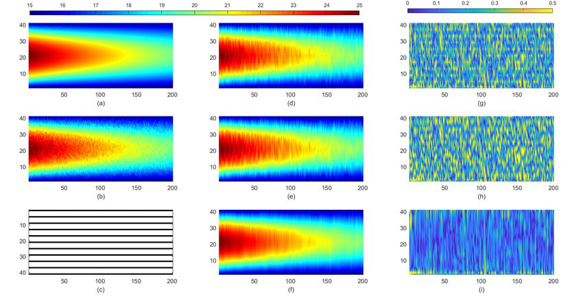
Appl. Sci. 2021, 11, 9050                                                                                            2 of 22

                            interpolations [7]. However, this strategy may lead to some deviations, especially the lack
                            of consideration of spatio-temporal correlation uncertainties in describing local variations
                            of dynamic fields. Similarly, data errors can be eliminated by filtering or statistical analy-
                            sis, but this approach is mostly biased towards temporal or spatial dimensions. Various
                            commonly used methods have been applied to model spatio-temporal field, including
                            the Bayesian model [8], State Space model [9], and Kalman filter [10]. In practical applica-
                            tion, these spatio-temporal dynamic models often require sufficient or consistent available
                            sensor observations to achieve a balance between estimation accuracy and computational
                            burden. Therefore, developing an effective and flexible spatio-temporal dynamic field
                            modeling method from sensor observation data is essential.

                            Figure 1. General processing of spatio-temporal data.

                                 In this paper, we propose the FUKSS model, approximating the stochastic equation
                            of state representation. This model retains the characteristics of universal Kriging, and
                            uses best linear unbiased estimation (BLUE) [11] to reconstruct the estimation function.
                            By the recursion and calculation of the state equation, we obtain the recursive variables
                            and the calculation process, similar to the Kalman filter error correction. In this way, we
                            make use of universal Kriging analysis of spatial correlation, while maintaining the Kriging
                            calculation burden for each function in the sequence, in order to achieve the error recursive
                            correction of inconsistent data and the storage of consistent intermediate variables. In
                            essence, the algorithm is more biased to the Kalman-Kriging filtering model estimation
                            in the spatial domain; that is, the weight of the current data in the current spatial domain
                            estimation is increased, to some extent, in the calculation process. The result is similar to
                            the extension of the unbiased vector Kalman filter proposed by Kitanidis [12] to the Kriging
                            space domain.
                                 In FUKSS, the problems to be solved and main contributions can be summarized
                            as follows:
                            •    The estimation of general position is realized by the statistical characteristics of Krig-
                                 ing [13,14]. At the same time, the intrinsic random function (IRF) [15,16] is used to
                                 replace the variation function which requires prior statistics in the Kriging process,
                                 such that the whole model does not need prior information in the calculation process.
                            •    In the process of model calculation, a constant size state vector is maintained (the size
                                 being the number of sensors, N, in the sensor network) and the available sampling
                                 data nt at time t is obtained through the data selection matrix W t for correction and
                                 calculation. This method solves the problem of data inconsistency caused by different
                                 sampling data at different times. At the same time, for a constant extra space storage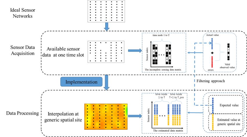
Appl. Sci. 2021, 11, 9050                                                                                                  3 of 22

                                 required (O( N 2 )) and computational complexity (O(n3t )) in the cyclic calculation
                                 process, the computational complexity can be further reduced by setting W t .
                            •    Through the derivation process, similar to that for a Kalman filter, the model real-
                                 izes a similar function to Kalman smoothing [17], such that the estimated data can
                                 eliminate the random systematic error, to a certain extent. Exponential smoothing
                                 prediction [18,19] is introduced, in order to improve the prediction ability of the model.
                                   The remainder of this article is organized as follows: Section 2 provides related
                            background information. Section 3 describes the FUKSS model in detail. For this model, in
                            Section 3.1, we propose the state equation and derive the recursive equation. A specific
                            formulation of the state-space model is described in Section 3.1.2, while the detailed
                            calculation process is described in Section 3.1.3. In Section 3.2, we describe the selection of
                            various functions for our model in detail. In Section 3.3, we introduce cubic exponential
                            smoothing prediction to realize the multi-step prediction by the model. Based on this
                            model, we conclude the paper with some numerical examples in Sections 4.1 and 4.2, an
                            application of the algorithm in Section 4.3, and a discussion of the method in Section 5.
                            Section 6 presents the conclusion of our work.
                                   Notations: Matrices are in upper case bold, and column vectors are in lower case bold.
                            The notation (.) T is the transpose operator, Zbt ( x ) is the estimate of Zt ( x ). The special cases
                            to be noted are: the regional variable functions Z and Y based on the stochastic process.
                            Zt ( x ) and Yt ( x ) represent an implementation of a random process at time t and position
                            x. In this case, bold capital Z t and Y t represents positions ( x1 , x2 , . . .) at time t, which
                            represents the n ∗ 1 vector. Sampling data lowercase x represents the position information
                            of a point, and a capital X represents the data set composed of n sampling points. An
                            identity matrix of size N ∗ N is denoted by I. k x a − xb k2 represents the second order
                            universal number between x a and xb , namely the Euclidean distance. Specific variable
                            settings in the manuscript can be found in Nomenclature part.

                            2. Related Work
                                 Estimation of arbitrary positions in space and time and filtering of observed data are
                            also being encouraged in other fields. In these application fields, estimation methods are
                            required as the main means to recover unknown information and solve the problems of
                            missing data, sensor layout optimization, sensor system error and so on. It also provides
                            support for data summary and spatial correlation study of observed data. In practice,
                            estimation methods are needed to process spatio–temporal dynamic data, potentially in
                            stream scenarios. Two common studies are mainly found in the literature as follows:

                            2.1. Kalman Filter
                                  Kalman filter is widely used in spatio-temporal dynamic modeling. In recent years,
                            Kriging has elicited considerable attention in describing spatial correlation, and has been
                            widely used to compensate for spatial correlation of Kalman filter, namely Kalman-Kriging
                            filtering model (KKF).
                                  In KKF, Kriging interpolation is used to construct a spatial field, in order to describe the
                            spatial correlation, and Kalman filtering is used to describe the temporal correlation [20–22].
                            Although Kriging [23–25] has been widely used to consider various fields of spatial correla-
                            tion, in KKF, the time dimension as an additional dimension, brings non-stationary changes,
                            that greatly increase the computational complexity of the linear equations. Considering the
                            large computation problem, the KKF model is suitable for the interpolation of spatial sparse
                            stations. Therefore, many researchers try to model covariance functions to reduce compu-
                            tational complexity, and several effective methods have been obtained, mainly including
                            sparse matrix algorithm, rank reduction technology, and Gaussian random field. For ex-
                            ample, Wike [26] proposed a space-time Kalman filter which has the dimension reduction
                            function and a temporally dynamic and spatially descriptive statistical model. Cressie
                            et al. [27–29] proposed a fixed-rank spatiotemporal Kalman, Spatio-Temporal Random
                            Effects, or Spatio-temporal Mixed-Effects model to calculate massive spatiotemporal data.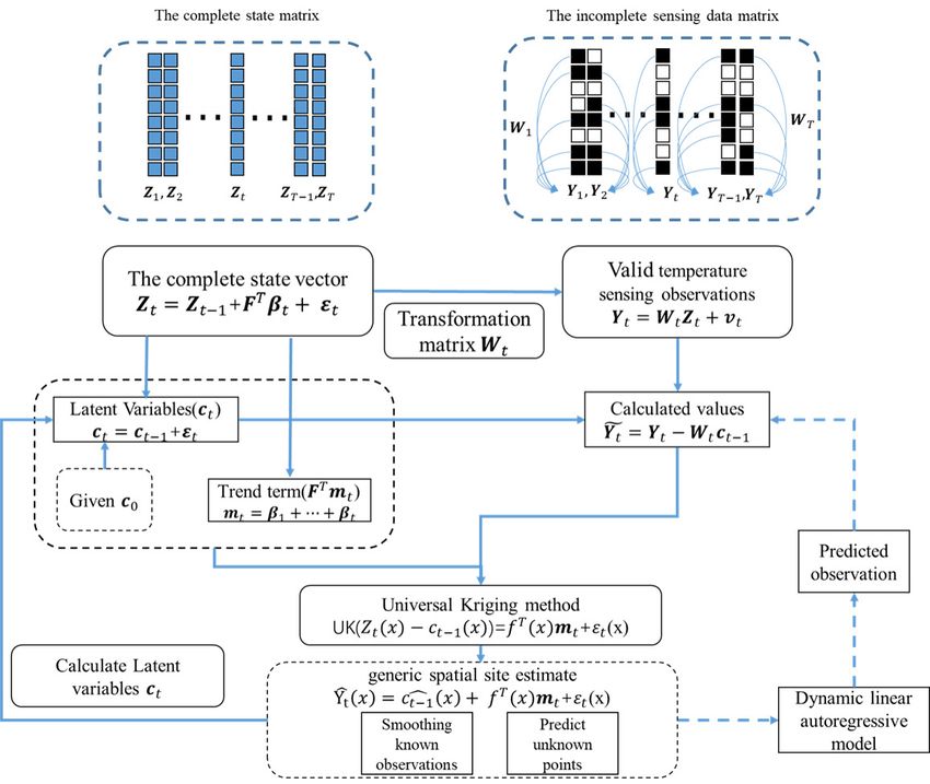
Appl. Sci. 2021, 11, 9050                                                                                           4 of 22

                                  As mentioned above, the KKF model has the advantages of Kriging and can also have
                            high interpolation accuracy for sparse sites or irregular sampling distribution. However,
                            the current calculation process of the KKF model [30] requires a lot of time to try different
                            initial parameters, in order to obtain the optimal accuracy, which limits the usefulness and
                            reliability of the model.
                                  In addition, the aforementioned method requires sufficient available sensor observa-
                            tions to achieve a balance between the accuracy of the field estimate and the computational
                            burden. This is mainly because the state vector and the observation vector need to be
                            consistent in the time dimension in the KKF process. However, one of the challenges in
                            modeling is that limited and time-varying distributions of sensor observations are avail-
                            able (sampling data at different moments are distributed differently, as shown in the data
                            acquisition in Figure 1).

                            2.2. State-Space Model
                                  The State-space model is also a rapid and flexible generalized model for handling a
                            wide range of spatio–temporal dynamic problems. In the state-space, a state transition or
                            state correlation model is constructed using stochastic theory, and then the transition or
                            correlation model is used to estimate the value of the unobserved spatio–temporal position.
                                  The state-space model based on Kriging can effectively use the characteristics of both.
                            As often happens in geostatistics, the Kriging state-space model also constructs the random
                            field into time-dependent trend terms and residual fields, where the trend term is used to
                            describe large-scale variation characteristics and the residual field is used to compensate
                            for local variation. The universal Kriging state-space model [3] has been used for the spatial
                            interpolation of medical images, and the error is corrected according to a Kalman filter of
                            time observations. The results of this model provide an optimal predictor for this process
                            decomposition and provide a basis for extending recursive filters to the spatial domain
                            of Kriging theory. Cressie [31] constructs Kriging state-space model using six-parameter
                            quadric in polynomial trend surface analysis. Martin [32] construct the Kriging state model
                            of the power trend using Euclidean distance, thus realizing the estimation of arbitrary
                            point sources at different times.
                                  However, this model does not take further advantage of the characteristics of the
                            universal Kriging method, which also requires the consistency of the observed data. At
                            the same time, due to the limitations of its algorithm, it cannot carry out prediction in the
                            absence of state inputs from the system. However, compared with the KKF algorithm, the
                            universal Kriging state-space model requires less prior knowledge.

                            2.3. Problems and Solutions
                                 Missing data and noisy data are problems encountered repeatedly in data acquisi-
                            tion and analysis. Especially for the analysis of spatio–temporal dynamic data, we also
                            need to consider the characteristics of time, space and space-time. Here, periodic sensor
                            temperature data obtained from grain storage is taken as an example to illustrate the data
                            challenge. Due to cost and mechanized operation constraints, a large granary has only
                            limited sensor observations (the distance between two adjacent horizontal sensors can be
                            up to 5 m). Sensor observations may not be properly collected into the database due to
                            unexpected reasons, such as sensor damage, communication failures, and data read/write
                            errors. In addition, the data obtained by the sensor not only has the detection error of
                            the sensor, but also has the systematic error caused by its principle, i.e., the temperature
                            obtained by the sensor is the temperature in the pore inside the grains instead of the actual
                            temperature of the grains. At the same time, this kind of data have obvious temporal and
                            spatial relationships, i.e., its temperature changes are continuous in time and correlated
                            in space.
                                 In general, there are three problems related to the automatic processing of collected
                            data: (1) The inconsistency of periodically collected data; (2) Possible deviation between
                            the observed value and the real value; and (3) problems related to the temporal collected
Appl. Sci. 2021, 11, 9050 5 of 22
data and historical data. For the above problems, the existing models require consistent
observations in the spatial and temporal domains to estimate dynamic fields. Compara-
tively, Kalman filter needs more data for pre-processing to obtain the initial parameters of
the model, so it has a better prediction structure than the state-space model. In order to
simplify the calculation, the proposed model is based on the state-space model, so it does
not need additional data for pre-processing.
The FUKSS proposed in this paper provides a cyclic estimation method for spatio-
temporal dynamic fields. The data selection matrix W t is used to realize the correspondence
between the state matrix and the observation vector, so that the observation data of different
sizes at different times can be directly used in the circular calculation process without
additional operation. At the same time, we use the universal Kriging feature to estimate
the arbitrary position and eliminate the system random error in a way similar to Kalman
filter. Finally, exponential smoothing prediction is introduced to obtain quasi-observed
value to simulate state input, so as to improve the prediction ability of the model.
3. Materials and Methods
3.1. Methodology
3.1.1. The FUKSS Model
The FUKSS model is based on a universal Kriging state-space model and introduces
the observed data Y t with length nt of different quantities and distributions into the cyclic
calculation process. In the calculation process, we maintain a constant state vector Z t with
length N and make corrections through different observation vectors. The FUKSS model is
described by the following state and measurement equations:
Z t = Z t −1 + F T β t + ε t , (1)
Y t = W t Z t + vt , (2)
where Z t = [ Zt ( x1 ), . . . , Zt ( xn )] T are the state values at N sensor nodes positions, and vt
is a vector of observation noise (nt ∗ 1), as determined by the measurement error of the
sensor. We can determine that vt = [vt ( x1 ), ..., vt ( xnt )] is white noise so that E[vt vtT ] = Rt ,
and it is uncorrelated with all past noise and data. F T βt is the expected value, where
F = [ f ( x1 ), . . . , f ( xn )], βt = [ β t1 . . . β tr ] T and f ( x ) = [ f 1 ( x ) . . . f r ( x )] T . Among them
f ( x ) denoting the r known drift functions, which often used in universal Kriging [33,34]
estimation, and βt is unknown drift coefficients vector (r ∗ 1). εt = [ε t ( x1 ), . . . , ε t ( xn )], ε t ( x )
denotes the spatially correlated errors, with zero mean and known covariance function:
E[ε t ( x a )ε t ( xb )] = k ( x a , xb ). (3)
In the calculation process, we introduce the selection matrix W t with size nt ∗ N
and rank nt . For a sensor network with N sensor nodes, all sensors are numbered to
obtain a vector for facilitate calculation. Therefore, the T rounds data collection will form
a measurement matrix, as shown in Figure 1. Here, each row of W t has only one 1 and
the rest of the entries are 0, where W t (i, j) = 1 representing the ith data Yt ( xi ) of Y t in the
coordinate of measurement matrix is j at time t. The expression is:
1, The ith node of Y t in the coordinate of sensor network is j.
W t (i, j) = (4)
0, otherwise
The essence of the FUKSS model is to maintain a fixed state variable Z t , and use a
different number of observation variables Y t to calibrate and estimate Zt ( x ), in order to
realize estimation of the whole process. In this model, the current state, Zt ( x ), is determined
by the previous state Zt−1 ( x ) and the stochastic model f T ( x ) βt + ε t ( x ) used in universal
Kriging. Therefore, we can obtain the estimated for a generic spatial site x, as follows:Appl. Sci. 2021, 11, 9050 6 of 22
bt ( x ) = Z
Y bt ( x )
T (5)
= Zt−1 ( x ) + f ( x ) βt + ε t ( x ).
b
3.1.2. Simplified Calculation
When working with this model, although the state equation is effective, it is difficult
to further calculate the Kalman filtering process. Therefore, we expand the state equation
and carry out some related simplifications:
Z t = Z 0 + ε1 + · · · + ε t + F T β1 + · · · + F T β t , (6)
c t −1 = Z 0 + ε 1 + · · · + ε t −1 , (7)
m t = β1 + · · · + β t . (8)
Using these definitions, Z t can be written as
Z t = c t −1 + F T m t + ε t . (9)
By definition, we know that the trend term F T mt provides the mean, and the first
component ct−1 = ct − εt is a latent variable representing the error. Therefore, we can
obtain the same expression as the spatial universal Kriging method:
KrigingEstimate( Z t − ct−1 ) = F T mt + εt . (10)
In contrast, the effective values we use for the universal Kriging estimate can be
expressed as:
e t = Y t − W tb
Y c t −1 . (11)
It is inevitable that we consider the change of the state equation at different times.
Our model is based on the state of the previous value and introduces a universal Kriging
estimate; the specific process is shown in Figure 2. As can be seen from the figure, our
model is mainly divided into two parts: One is the latent variable ct representing the errors,
and the other is the trend term F T mt . In the model, we use the current observation data to
simulate the trend term, and use the method similar to Kalman filter derivation to carry
out correction and progressive estimation of latent variable. Therefore, the essence of this
model is to update and cyclically estimate the error after removing the known trend term.
For the sake of consistency, we assume that neither trend term F nor Systematic error
distribution Rt changes with the time t. For spatially correlated errors ε t ( x ) at different
times, we assume that:
E[ε t1 ( x a ), ε t2 ( xb )] = 0, t1 6= t2. (12)
Finally, as an initial condition, we assume that Z 0 is a zero-mean process with a
covariance function aE[ε0 ε0T ], in order to keep ct consistent over time. Where a is a known
parameter. Thus, we can extrapolate that Z0 ( x ) is not correlated with ε t ( x ) for all t from
the hypothesis.The next part of this article details the derivation and lists the required
leading parameters.Appl. Sci. 2021, 11, 9050 7 of 22
Figure 2. Flexible Universal Kriging state-space model flow chart.
3.1.3. Recursive Estimate
Given the observed data Y t and the latent variable b
ct−1 at time t, we estimate Zt ( x ) to
bt ( x ). In this case, we use BLUE, which is widely used in universal Kriging, with
obtain Y
expression by Equation (11):
bt ( x ) = cbt−1 ( x ) + q T ( x )Y
Z et. (13)
t
bt ( x )] = E[cbt−1 ( x ) + q T ( x )Y
Unbiasedness implies that the estimate must satisfy E[ Z et] =
t
T
f ( x )mt , which leads to the constraint
FW tT qt ( x ) = f ( x ). (14)
The best estimate Z bt ( x ))2 ],
bt ( x ), then minimizes the mean squared error E[( Zt ( x ) − Z
subject to the constraint
2 = E [( Z ( x ) − c
σez t bt−1 ( x ) − qtT ( x )Y
e t )2 ]
T
= E[(ε t ( x ) + ct−1 ( x ) + f ( x )mt − cbt−1 ( x ) − ... (15)
T
qt ( x )(W t εt + W t ct−1 − W tb c t −1 + W t F T m t + v t )2 ] .
Squaring the argument and applying the expectation yields
2 = σ2 ( x ) + σ2 ( x ) + q T ( x )(W P T T
σez ε c t t t−1 W t + W t KW t + Rt ) qt ( x ) − ...
T (16)
2qt ( x )W t ( pt−1 ( x ) + k( x )).
where
σε2 ( x ) = E[(ε t ( x ))2 ], (17)
σc2 ( x ) = E[(ct−1 ( x ) − cbt−1 ( x ))2 ], (18)Appl. Sci. 2021, 11, 9050 8 of 22
pt−1 ( x ) = E[(ct−1 ( x ) − cbt−1 ( x ))(ct−1 − b
ct−1 )], (19)
Pt−1 = E[(ct−1 − b c t −1 ) T ] ,
ct−1 )(ct−1 − b (20)
k ( x ) = E [ ε t ( x ) ε t ], (21)
T
K = E [ ε t ( ε t ) ]. (22)
In this result, we know that vt is white noise, such that its expectation with the other
values is 0. The terms qtT ( x )W F T mt and f T ( x )mt can be removed from the expression by
Equation (14). Thus, the question now is how to compute qt ( x ). The qt ( x ) is derived by
minimizing the variance of the prediction error, subject to FW tT qt ( x ) = f ( x ), such that the
prediction is unbiased. The constrained minimizing the variance problem can be solved by
the Lagrange multiplier method:
2
ξ ( x ) = σez + λ T FW tT g t ( x ), (23)
where the Lagrange multipliers λ are unknown and must be estimated. Setting the partial
derivatives of this criterion with respect to g t ( x ) and λ equal to zero, we obtain the
following equations:
2(W t Pt−1 W tT + W t KW tT + Rt )qt ( x ) − 2W t ( pt−1 ( x ) + k( x )) + W t F T λ = 0
. (24)
FW tT qt ( x ) = f ( x )
Therefore, we can solve for qt ( x ), yielding the desired minimizing weight vector
qt ( x ) = ( I − M tT FW t ) Lt W t ( pt−1 ( x ) + k( x )) + M tT f ( x ), (25)
where
Lt = (W t Pt−1 W tT + W t KW tT + Rt )−1
. (26)
M t = ( FW tT Lt W t F T )−1 FW tT Lt
As all K and Rt are positive definite, and this implies that the inverse exists. Pt is
positive semi-definite covariance matrices, and Lt is also positive definite. Then, we can
prove that FW tT Lt W t F T is full rank and has rank r because we have assumed F has rank r.
This implies that M t exists.
By the generalized least squares method we can obtain the unknown drift coefficients
vector mt in Equation (10):
mt = M t Y
et. (27)
ct and cbt ( x ) by the following equations:
Thus, we can obtain the estimates of b
ct = Zb t − F T mt
(28)
b
= bct−1 + (Pt−1 + K )W tT Lt ( I − W t F T M t )Yet ,
bt ( x ) − f T ( x ) m t
cbt ( x ) = Z
(29)
= cbt−1 ( x ) + ( ptT−1 ( x ) + k T ( x ))W tT Lt ( I − W t F T M t )Y
et.
Let G t = (Pt−1 + K )W tT Lt ( I − W t F T M t ) and g t ( x ) = ( I − M tT FW t ) Lt W t ( pt−1 ( x ) +
k( x )). Then, we obtain
ct = b
b c t −1 + G t Y
et, (30)
b ct−1 ( x ) + g tT ( x )Y
ct ( x ) = b et. (31)
ct ,
Before estimating these unknown terms, we can obtain a recursive estimate, b
as follows:
T
ct =
b ∑ Gi Ye i , (32)
i =1Appl. Sci. 2021, 11, 9050 9 of 22
T
ct ( x ) =
b ∑ g iT (x)Ye i . (33)
i =1
Then, we evaluate Pt , as in Appendix A:
Pt = (Pt−1 + K )( I − W tT G tT ). (34)
To achieve the unknown quantity pt−1 ( x ), we discuss the relationship between
pt−1 ( x ) and k( x ) further in Appendix B, and obtain:
p t −1 ( x ) = P t −1 K −1 k ( x ). (35)
We yield the solution between g t ( x ) and G t :
g t ( x ) = G tT K −1 k( x ). (36)
The solution in Equation (33) we can also be written as:
cbt ( x ) = k T ( x ) ∑it=1 K −1 Gi Y
ei
T − 1 . (37)
= k ( x )K bct
Therefore,
Zbt ( x ) = cbt−1 ( x ) + q T ( x )Y
et
t
T T
= cbt−1 ( x ) + g t ( x )Y e t + f ( x )mt
T − 1 T . (38)
= k ( x )K bct + f ( x ) M t (Y t − W tbct−1 )
= k T ( x )K −1bct−1 + k T ( x )K −1 G t (Y t − W tbct−1 ) + f T ( x ) M t (Y t − W tbct−1 )
Finally, we use the equation in Equation (5) to write:
bt ( x ) = k T ( x )K −1b
Y c t − 1 + k T ( x ) K − 1 G t (Y t − W t b
c t − 1 ) + f T ( x ) M t (Y t − W t b
c t −1 ). (39)
3.2. Recursive Estimation and Parameters Settings
Our algorithm has a lot of prior variables, as shown in the previous derivation;
mainly K, k( x ), P0 , Rt , and F. First, the parameter selection of Rt is mainly based on
the measurement error of the observation itself. Therefore, the observed quantities are
independent of each other. Therefore, for Rt , we need the corresponding probability
distribution to obtain the variance.
Second, we can find the value of P0 = TK using the length of the sample data, or we
can just specify the value of P0 = 0 or a smaller value, when T is large.
Third, we must specify drift functions to obtain f ( x ) and F, mainly to reflect spatial
non-stationarity. However, as the specific order of the spatial trend distribution cannot
be obtained, the lower order is generally chosen to reflect the possible spatial trend char-
acteristics, and the experiment proves that this choice also obtains good results. In fact,
this phenomenon also conforms to the characteristics of universal Kriging estimation. In
the process of universal Kriging estimation, it is necessary to calculate the variogram or
covariance function of the residual error by removing the drift term. Compared with the
calculation without drift term, the result can be made more accurate by removing the trend
term of lower order.
Finally, it is difficult to choose the general k( x a , xb ) in Universal Kriging theory, to
determine K and k( x ). To simplify the calculation, we chose intrinsic random functions
(IRF), which are a more generalized covariance function. In this paper, we propose two
generalized covariance functions. Matheron [15] proposed an IRF model of order k, with
+1
expression k(k x a − xb k2 ) = k x a − xb k2k
2 . Watson [16] proposed an IRF function similar
to a spline, with expression k(k x a − xb k2 ) = k x a − xb k22 logk x a − xb k2 . Therefore, the
form of k( x a , xb ) in this paper mainly refers to these two forms, and good results wereAppl. Sci. 2021, 11, 9050 10 of 22
obtained in the experimental verification. The specific steps are provided in Algorithm 1.
As shown in table, this FUKSS model maintains a fixed-size state variable ct and transfer
matrix Pt . The complexity of calculation at time t is only related to the quantity of valid
sampling data Y t .
Algorithm 1: FUKSS Algorithm
Initialize: t = 1, P0 = αK, c0 = 0(n ∗ 1).
Given: K, k ( x ), α, Rt , F, Wt
State equations:
Zt ( x ) = Zt−1 ( x ) + f T βt + ε t ( x )
Observation equation:
Yt ( x ) = Zt ( x )
For t = 1, . . . , T
Calculate the matrices:
Lt = (W t Pt−1 W tT + W t KW tT + Rt )−1
M t = ( FW tT Lt W t F T )−1 FW tT Lt
G t = (Pt−1 + K )W tT Lt ( I − W t F T M t )
Calculate the desired estimate using:
bt ( x ) = k T ( x )K −1b
Y ct−1 + (k T ( x )K −1 G t + f T ( x ) M t )(Y t − W tb
c t −1 )
Updated parameters :
Pt = (Pt−1 + K )( I − W t G tT )
ct = b
b c t − 1 + G t (Y t − W t b
c t −1 )
end
3.3. Dynamic Linear Autoregressive Model Specification
The prediction ability discussed in this paper is mainly for multi-step prediction ability.
In this experiment, the time interval between the time-series data is equal, and the current
data are used for estimation and revised in our calculations. Therefore, this method is
not suitable for prediction, due to the lack of a specific model to exclude the prediction
of future functions. Compared with spatial interpolation, our model can eliminate the
observation error, to a certain extent, with an operation similar to that of a Kalman filter.
To solve this problem, we introduce the dynamic linear autoregressive model to solve the
prediction problem. During prediction, the predicted value is closer to the current value,
as illustrated in the subsequent tests.
A simpler alternative model, based on the dynamic linear model, is the Holt–Winters
model. This model has three main components: A smoothing sequence (St ), a trend
sequence (Bt ), and a periodic smoothing sequence (C t ). We can combine these components
together with several methods. To make the model more general, we use an additive model,
which integrates the components together to obtain the full model.
Y t +1 = S t + B t + C t − L +1 , (40)
where L is the length of periodic sequence. Inside the model, we use the cubic exponential
smoothing method to yield the components. ζ, τ, and γ are the parameters used, which
have values between 0 and 1. The equations are given below.
Y ct−1 + ( G t + F T M t )(Y t − W tb
bt ( X ) = b c t −1 ), (41)
bt ( X ) − C t− L ) + (1 − ζ )(St−1 + Bt−1 ),
S t = ζ (Y (42)
B t = τ ( S t − S t −1 ) + (1 − τ ) B t −1 , (43)
bt ( X ) − St ) + (1 − γ)C t− L .
C t = γ (Y (44)
The initial data have little impact on the whole model, so we choose S0 = Y
b0 ( X ),
b1 ( X ) − Y
B0 = Y b0 ( X ), and Y
b0 ( X ) = 0.Appl. Sci. 2021, 11, 9050 11 of 22
We introduce exponential smoothing prediction to provide additional quasi-observable
values for multi-step prediction. The detailed steps are shown in Algorithm 2. Exponen-
tial smoothing prediction is introduced to enhance FUKSS multi-step prediction. In the
prediction process, we first use our proposed model to re-estimate the observed values,
in order to improve the accuracy of exponential smoothing prediction, which can realize
data cleaning (e.g., denoising) to a certain extent. For the prediction stage, we use the
updated parameters of the iteration to re-estimate the quasi-observed values, which makes
the actual predicted value more in line with the spatial distribution law set by the model.
However, this prediction error also increases with the increase of the prediction step size.
At the same time, due to the limitation of the dynamic linear model, it can predict and
describe the time-series with trend and periodic change more accurately.
Algorithm 2: FUKSS Prediction algorithm
Initialize: t = 1, P0 = αK, c0 = 0( N ∗ 1).
Given: K, k( x ), α, Rt , F,W t ,Tpre , L, ζ, τ, and γ
For t = 2, . . . , T
Loop calculate the matrices: Lt , M t , G t , Pt , cbt
Calculate the desired estimate using:
Ybt ( X ) = b ct−1 + ( G t + F T M t )(Y t − W tb c t −1 )
Calculate the dynamic linear autoregressive parameters:
S t = ζ (Y bt ( X ) − C t− L ) + (1 − ζ )(St−1 + Bt−1 )
B t = τ ( S t − S t −1 ) + (1 − τ ) B t −1
C t = γ (Y bt ( X ) − St ) + (1 − γ)C t− L
End for
For t = T + 1, . . . , Tpre
Yt ( X ) = St−1 + Bt−1 + C t− L
Ybt ( X ) = b ct−1 + ( G t + F T M t )(Yt ( X ) − b
c t −1 )
According to the order calculate the corresponding parameters:
Lt , M t , G t , Pt , b
ct , St , Bt , C t .
End for
4. Experiments
In this section, we present experimental comparisons of different types and dimen-
sions. First, we conducted experiments on a thermodynamic fitting data set, in order to
demonstrate some of the model’s characteristics, including accuracy, continuous estimates
of different sampled data, and prediction ability. We also apply the FUKSS model to
real data.
4.1. Experiments on Thermodynamic Model
There have been many studies on thermal spreading models in the field of spatio-
temporal analysis and prediction [35]. In the aspect of spatio-temporal correlation, they
have very obvious characteristic. At the same time, their complexity is manageable. A 1D
simple thermodynamic model is:
∂2 T ∂T
a( )= , (45)
∂x2 ∂t
where T is the temperature field, including time t and position x, and a is the thermal
conductivity coefficient.Using the finite difference method, it can be discretized as
( Tti−1 − 2Tti + Tti+1 )
Tti+1 = Tti + a∆t , ∀i ∈ 1, . . . , n. (46)
∆x2
The time of thermodynamic simulation was 200 time steps, and 41 discrete points
were selected for calculation to construct the data set. The initial temperature distributionAppl. Sci. 2021, 11, 9050 12 of 22
was 25 − 40 ∗ ( x − 0.5)2 , which is a second-order distribution, and the boundary conditions
were fixed. The result is shown in Figure 3a. White noise with a standard deviation of
σ = 0.5 was also added to the simulated data, the results are shown in Figure 3b. We evenly
chose 10 points in the interval at which to observe the functions. The sampling model is
shown in Figure 3c.
We applied the FUKSS with model parameters k ( x a , xb ) = k x a − xb k32 , f ( x ) =
[ 1, x ] T , Rt = 0.52 I, and α = 5. In the actual work process, we often cannot determine
the trend term order of the distribution, and generally choose a low possible order. There-
fore, we chose first-order f ( x ) in this experiment, and proved that this choice also achieved
good results. For the parameter Rt , we chose the observation error as a Gaussian distribu-
tion with standard deviation of 0 and variance of 0.52 . The selection of other parameters is
detailed in Section 3.2 and the discussion.
The resulting function estimates are depicted in Figure 3f. The same sampled data
were used in linear and Kriging. Note, that we adopted the same covariance parameter as
FUKSS, as the fitting of the covariance function could not accurately describe the actual
situation due to the small amount of sampling data for Kriging interpolation. Compared
with the experiment, we found that the three methods could fit the actual situation well, but
the proposed method had a smaller error. At the same time, it can be seen, from Figure 3f,
that the Kalman filtering method could effectively eliminate the observation noise.
Figure 3. Heat diffusion data at 41 points and 200 time-steps: (a) Ground truth; (b) Noisy data
derived from the real; (c) Sample of the noisy data; (d) Estimates using linear model; (e) Estimates
using Kriging model; (f) Estimates using the proposed algorithm; (g) Deviation of the linear model
estimate from the true value; (h) Deviation of the Kriging model estimate from the true value; and (i)
Deviation of our model estimate from the true value.
We further compared different sampled data at different times, and the results are
shown in Figure 4. Different sampling methods had an obvious influence on the spatial
interpolation but, through iteration, our model obtained better results, compared with the
other spatial interpolation models. At the same time, comparing Figures 3f,i and 4f,i, under
the condition of the same number of observable sensors, multiple sampling methods can
improve the fitting accuracy of the model.
In Figure 5, we took out 40 time-steps equally from 200 time-steps, in order to simplify
the calculation process. The first 30 time-steps were trained and the last 10 time-steps were
used as prediction test. We applied the KUKF Prediction algorithm with cubic exponential
smoothing model parameters ζ = 0.8, τ = 0.3, γ = 0.2, and L = 0. For Figure 5e, we
chose this model instead of KKF, mainly as the Kalman filter cannot be corrected when
making multi-step prediction, which will increase the error and does not conform to theAppl. Sci. 2021, 11, 9050 13 of 22
usage of the Kalman filter itself. As for Figure 5f, we used FUKSS to make the data similar
to Kalman smoothing, improving the prediction result of the dynamic linear model. This
method optimizes the Kalman filter correction problem in multi-step prediction, to a certain
extent. However, at the same time, the model is required to have a more suitable initial
parameter setting, which makes the model establishment more difficult.
Figure 4. Heat diffusion data at 41 points and 200 time-steps: (a) Ground truth; (b) Noisy data
derived from the real; (c) Sample of the noisy data; (d) Estimates using linear model; (e) Estimates
using Kriging model; (f) Estimates using the proposed algorithm; (g) Deviation of the linear model
estimate from the true value; (h) Deviation of the Kriging model estimate from the true value; and
(i) Deviation of our model estimate from the true value.
Figure 5. Heat diffusion data at 41 points and 40 time-steps: (a) Ground truth; (b) Noisy data derived
from the real; (c) Sample of the noisy data; (d) A training area; (e) Estimates using Holt-Winters
model with training area; (f) Estimates using the proposed algorithm with sampled the noisy data;
(h) Deviation of the Kriging spatial model estimate from the true value; and (i) Deviation of our
model estimate from the true value.Appl. Sci. 2021, 11, 9050 14 of 22
4.2. 2D Function Simulation
For the external variation conditions, we also carried out relevant experimental veri-
fication. Figure 6a shows a two-dimensional thermodynamic conductivity diagram, the
bottom of which has a fixed temperature value, where the external temperature varies
with time, and different thermal conductivity coefficients in the X and Y directions are
used. We imitate the basic coefficient of grain storage, where the length was 24 m and the
height was 7 m. The thermal conductivity referred to the actual thermal conductivity of
wheat in the actual storage. The initial condition was set as uniform temperature, and we
conducted 360 simulations with days as the unit of time. The external conditions were
fitted into the annual weather changes using a second-order function. Sampling points
are set using a grid sampling method with six points in the X direction and five points
in the Y direction. In addition, we randomly selected 90% of the data at all sampling
points for each time period. We resampled the time-series on a seven-day basis, in order
to obtain 50 time-series with sampling intervals of weeks. Taking the first 40 as training,
we predicted the temperature of the 45th. We added noise to the sampled data, using is a
random distribution with a standard deviation of 0.5. The parameters selected for fitting
were as follows:
k ( x a , xb ) = k x a , xb k22 logk x a , xb k2 , f ( x ) = [ 1, x, y] T (47)
Figure 6. 2D sequence temperature simulation (times 1, 12, 23, 34 and 45 are shown): (a) Temperature
simulation; (b) Fit by FUKSS; and (c) Fit by radial basis interpolation.
We chose Rt = 0.52 I and a = 40. Figure 6b was obtained using our model. Figure 6c
shows radial basis interpolation [36], where the radial basis function is:
f ( x a , xb ) = k x a , xb k22 (logk x a , xb k2 − 1) (48)
As can be seen from Figure 6, the changes of external conditions were described more
accurately using the proposed model. In particular, at t = 23, a small bull’s-eye region
appears obviously in the radial basis function fit, mainly caused by the random error of
sampling. In our model, there was obvious consistency between the before and after, and
the timing prediction with five steps was also described more accurately.
The grain storage process is mainly affected by external weather conditions, which
mainly present periodic changes. Therefore, we used the dynamic linear regression method
to strengthen the multi-step prediction and obtain relatively more realistic results. At the
same time, the spontaneous heat conduction inside the grain pile forms the distribution
pattern of hot and cold zone, for which the Universal Kriging method can provide a more
accurate description. Therefore, the prediction model can provide more accurate descrip-
tion and prediction for the grain storage process. In contrast, this linear regression modelAppl. Sci. 2021, 11, 9050 15 of 22
conducts multi-step prediction mainly for spatio-temporal data with periodic changes in
the boundary conditions.
To further verify the reliability of our model, we used signal data to carry out fitting,
in which changes in the temporal characteristics are more common. First of all, we used
a sinc function to generate a time signal, and added spherical information on this basis,
such that the simulation data contained spherical coordinate information and sinc function
time information. As shown in Figure 7a, the height of the sinc function increased over
time. We intercepted data from 25 equal time intervals, each of which was sampled on an
equally spaced grid. Moreover, we added white noise to it, where the standard deviation
was 0.1 times the maximum signal value of the whole process. The first 20 intervals were
used for training and the last 5 were used for prediction.
Figure 7. 2D sequence signal simulation (times 1, 6, 11, 16 and 21 are shown). (a) Original signal
functions without white noise; (b) Fit by FUKSS; and (c) Fit by Smoothing thin-plate spline.
To estimate the original function from the noisy data, we applied the Kriging filter
with data covariance function and the drift functions (according to Equation (47)). In this
case, we chose Rt = σ2 I and a = 20. The results are shown in Figure 7b. For further com-
parison, cubic spline interpolation was selected for interpolation analysis of the sampled
data, for which the results are shown in Figure 7c. Cubic spline interpolation preserves
the advantages of piecewise interpolation polynomials and improves the smoothness of
interpolation functions. However, as the sampling data contained noise, there were large
fluctuation when cubic spline interpolation is used. Comparing (b) and (c) in Figure 7, both
methods can preserve the characteristics of the original simulation to a certain extent, but
the proposed model had smoother results, compared with cubic spline interpolation [37].
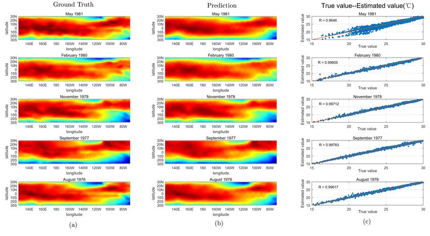
4.3. Application to Real Data
The Pacific Sea Temperature (PST) data set, which can be obtained from the Climate Data
Library at Columbia University (http://iridl.ldeo.columbia.edu/SOURCES/.CAC/, accessed
on 27 September 2021) [38], has 2520 sample temperature data points per month on the
Pacific from January 1970 through March 2003. The sampling mode is grid (84 * 30), with a
longitude and latitude interval of 2. In the PST data, the first 120 time-series were used for
training, and the observation error was set as 0.5. The data of the subsequent 24 months
were then predicted and described.The forecast period was 24 months, from January 1980
to December 1982. To estimate the PST, we first used data normalization to make the
coordinates in the same grade interval, and each time was resampled on a regular 21 ∗ 10
grid. We applied the Kriging filter with the data covariance function in Equation (47),
T
drift functions as f ( x ) = 1, x, y, xy, x2 , y2 , and cubic exponential smoothing model
parameters ζ = 0.45, τ = 0.2, γ = 0.95, and L = 12. The results are shown in Figure 8, whileAppl. Sci. 2021, 11, 9050 16 of 22
Figure 9 shows a comparison of the temperature of a single coordinate over time. As can be
seen from the two figures, our method achieved good results, could effectively predict the
temperature value of unknown points in the training data, and can also effectively show
the trend of change in the prediction process.
Figure 8. Temperature images from the PST data set. (a) Ground truth; (b) Estimates of the resampled
points using our algorithm; and (c) Predicted against resampled points for all real points.
It can be seen, from the experiment, that the training deviation was relatively small,
mainly due to the accuracy of universal Kriging estimation and Kalman filter using the
correction of the current observations. At this point, we introduce the dynamic linear
model to introduce additional quasi-observable values. Experimentally, it was found
that the introduction of such quasi-observable values in the multi-step prediction led to
better results. The possible reasons for this are as follows: (1) Kalman filtering cleans and
smooths the data in the time-series, by removing the possible noise or outliers, such that
better results can be obtained in dynamic linear prediction of the smoothed data; and
(2) during the simulation interpolation, universal Kriging also fitted the data with features
and correlations, in order to make the data more consistent with the actual situation.
Although we solved the multi-step prediction, to a certain extent, the error of the additional
quasi-observable values obtained by the dynamic linear model increases as the step size
of the prediction increased. At the same time, this quasi-observable value error is also
transmitted to the gain matrix, thereby increasing the error. In our choice of May 1981,
which is a five-step forecast relative to the time interval, we can clearly see the variation of
this error. The temperature of the Pacific Ocean changes on an annual basis. Although the
range of change in this cycle is not large, it is also shown in the single point chart. Generally,
the annual period of change is about 5 ◦ C, but that in some regions can also reach a range
of more than 10 ◦ C. This is something that we have not fully solved yet as, over time, these
errors accumulate and the forecast starts to drift. However, we still obtain high accuracy in
multi-step short-term forecasting.
The considered grain warehouse temperature test system was a generally distributed
system. The temperature sensor is stored in a cable, and fixed on the wall at one end. In
this way, a rather warehouse impression of the locations of temperature sensors could
be obtained. In this data, on the horizontal plane, the vertical and horizontal spacing
of temperature measuring points were 4.3 m and 4.6 m, respectively, with a total of six
rows and 11 columns, a height distance of 6.7 m, and a total of five layers. The sensor
arrangement is shown in Figure 10a. The data, mainly from October 2016, showed that it
cooled during the November period, until June 2017, the data were mainly temperature
data, and the collection time was once a week. To estimate grain warehouse temperature,Appl. Sci. 2021, 11, 9050 17 of 22
we used data from the first 10 weeks for training and predicted data from the 14th week.
From week 5, a small amount of sensor information was incorrectly collected and the value
is null. In weeks 7 and 8, information collection of the entire temperature measurement
cable was lost.
We applied the Kriging filter with the data covariance function in Equation (47),
drift functions as f ( x ) = [ 1, x, y, z] T , and cubic exponential smoothing model parameters
ζ = 0.8, τ = 0.5, γ = 0.3, and L = 0. In this case, we chose σ = 0.5 and a = 10. The results
are shown in Figure 10.
Figure 9. Time-series temperature changes at predicted and original points. Among them, the first
120 months were used for training and the next 24 months were predicted: (a) The resampled points;
and (b) the points estimated though our algorithm, using resampled points.
(a) A 3D sketch of grain temperature field in a (b) A six-view plot in 5th week
granary
(c) A six-view plot in 10th week (d) A six-view plot in 14th week
Figure 10. Analysis of grain temperature through our algorithm: (a) Distribution of sensors in the
grain storage silo; (b,c), the first 12 weeks were sampled data for gradual fitting; and (d) prediction at
the 14th week.
The granary temperature monitoring system is a three-dimensional storage system.
As such, this analysis was carried out in 3D, as showing in Figure 10b–d, with an expanded
view of the outer surface. Unsurprisingly, the change was not very dramatic, given the
huge size of the silo and the fact that bulk grains are poor conductors of heat. However,
for the temperature forecast from week 11 onwards, we obtain better results, as shown in
Figure 11. The reason for this lies in the particularity of grain storage. Grain storage isAppl. Sci. 2021, 11, 9050 18 of 22
mainly affected by external conditions and shows periodic changes, making it a suitable
scenario for the dynamic linear regression model.
Figure 11. Prediction against sampled points for all real points.
5. Discussion
The FUKSS model presented in this paper is a step-by-step method which can be
used to reconstruct the time-series of spatial functions from scattered data. As our model
is based on the universal Kriging state-space model, the calculation process is based on
Kriging’s spatial statistics and the derivation is similar to that of a Kalman filter. In terms
of space, we do not need to have strict distribution requirements for the sampled data.
Using the statistical characteristics of Kriging, partial missing or new data have little
impact on the estimate. In terms of time-series prediction, this model has the advantages
of small memory requirement (constant extra space storage required O( N 2 )), acceptable
computational speed (constant computational complexity O(n3t )), and being suitable for
dynamic problems. The keys to deducing the recursive filter is to use linear unbiased
estimation, establishing the optimality of the recursive formulation. This method uses not
only historical data but also the spatial relationship between the historical data, which
optimizes the results. To further solve the problem that it is impossible to make long-term
predictions, we introduce the dynamic linear regression model to carry out secondary
processing on the estimated value of each step, such that the spatial information can still
be retained, to some extent, in the long-term prediction. However, there are still some
limitations to our model.
As FUKSS is based on the universal Kriging state-space model, our algorithm can be
simplified to a similar method of universal Kriging interpolation and Kalman filtering in
special cases. If the sensor accuracy is not taken into account—namely, if the measurement
data is unbiased—we can simplify it, to a certain extent, to universal Kriging interpolation
fitting in this time period. If we do not consider the drift term in Equation (1), we can
simplify it to space–time Kalman filtering [39]. Therefore, the parameters of universal
Kriging and Kalman filtering are used simultaneously in our model, such that the model
has the advantages and disadvantages of both.
Our algorithm has a lot of prior variables; for example, we have to specify K, k( x ),
α, Rt , and F. The selection method for these parameters (except for a) is similar to that
of universal Kriging, which has been described in detail in the literature [31]. In general,
we recommend using a polynomial drift function for F, as discussed in the literature [40].
For K and k( x ), we cannot calculate them statistically as with universal Kriging, or fit it in
any other way, as they would take a lot of computational effort to determine. To simplify
the calculation, we chose IRF, which are a more generalized covariance function [15,16] .Appl. Sci. 2021, 11, 9050 19 of 22
If enough data points are available, the selection of the covariance function is not critical.
Finally, the noise covariance is mainly determined by the parameters of the sensor which
has an effect similar to the smoothing parameters of the smooth spline.
Compared with KKF, the advantage of our method is that it considers the development
law of dynamic system through the state space model, so it does not need to spend a lot of
prior calculation to obtain the initial parameters. However, in the calculation process of
KKF, the parameters are estimated from all historical data, which is more universal than our
algorithm. From the results, our model focuses more on temporal space, while KKF focuses
more on time. To estimate past values of the function, our method is similar to estimation
by Kalman smoothing, which can obtain a relatively good result. As the trend term F T mt in
our model is determined by the current sampling data Y t , our model is more unsuitable for
time prediction than KKF. Therefore, we introduced a dynamic linear regression into our
algorithm, in order to supplement the function of time prediction. At the same time, due to
the limitations of dynamic linear models, our multi-step prediction may be more suitable
for spatio-temporal data with periodic and trend changes. Comparing the simulation and
actual data, good prediction results were observed.
Some limitations of the FUKSS and its modified, as presented, is the assumption
regarding the initial parameters. First, we assume that c0 ( x ) is a zero-mean process with a
covariance function E[c0 ( x a )c0 ( xb )] = αk( x a , xb ). Of course, the known non-zero mean can
be obtained from all the data vectors, but this requires a lot of extra work for the general
covariance function. We chose [26], as it proposes two most likely cases, which do not add
significant complexity to the description of the algorithm. Those two cases are as follows:
(1) c0 ( x ) is known, such that α = 0; and (2) c0 ( x ) is determined by the definition, in which
case it can be simplified to the length of the running time. In practical application, we prefer
the second case, which is simulated as shown in Figure 4. On the other hand, we prefer to
take a smaller value than zero if enough data points are available. Second, our algorithm
takes advantage of the characteristics of Kriging space statistics and does not require fixed
observation points. For the additional sample data, the computation requirement of our
algorithm will be greatly increased. Finally, as for selecting parameters for dynamic linear
regression, we need prior knowledge to obtain better results, which can lead to extra
workload. Due to the characteristics of the cubic dynamic linear regression model and the
certain smoothing of the historical data by our FUKSS model, rough parameter selection
can be used to obtain relatively good results.
6. Conclusions
In this work, we proposed a spatio-temporal dynamic field estimation algorithm with
a bias toward spatial optimization, based on universal Kriging state-space model. This
model can describe the spatio-temporal characteristics of spatio-temporal data flexibly and
efficiently, and yield its interpolation or prediction accurately. The proposed method uses
spatial statistical information to reduce the requirement of sensor sampling consistency.
We introduced dynamic linear regression into our algorithm, in order to supplement the
function of time prediction. The salient features of this method include handling the spatial
covariance matrices and tackling measurement noise. Numerical comparison indicated
the feasibility and accuracy of the proposed method. Future research will consider how
to set up self-organizing networks in the deployed sensors using temporal and spatial
correlation, such that the service life of the sensors can be extended.
Author Contributions: Z.S. conceived the study and contributed to the design of the study, modeling,
data interpretation, drafted and revised the manuscript. X.Z. contributed to the development of
algorithms, data evaluation, and data analysis. All authors have read and agreed to the published
version of the manuscript.
Funding: This research received no external funding.
Institutional Review Board Statement: Not applicable.
Informed Consent Statement: Not applicable.Appl. Sci. 2021, 11, 9050 20 of 22
Data Availability Statement: Not applicable.
Conflicts of Interest: The authors declare no conflict of interest.
Nomenclature
N The ideal number of sensors.
nt Number of effective observed sensors at time t.
x Space position.
X Set of interested sites in quantity N.
Zt ( x ) State variables at location x and time t.
Yt ( x ) Observations at location x and time t.
Zt The state vector at time t for N sensors.
Yt Effective observed vector at time t for nt sensors.
bt ( x ), Z
bt ( x ) , Y
Z b t ( x ), Y
b t (x) Estimate of Zt ( x ), Yt ( x ), Z t ( x ), Y t ( x ), respectively.
Wt The selection matrix is used to represent the conversion relationship
between ideal sensors and effective observation sensors, and its matrix
size is nt ∗ N and its rank is nt .
f ( x ) = [ f 1 ( x ) . . . f r ( x )] T Known drift functions at location x with size r ∗ 1.
F = [ f ( x1 ), . . . , f ( xn )] Known drift functions at N ideal sensors location with size r ∗ N.
βt = [ β t1 . . . β tr ] T Unknown drift coefficients vector at time t with size r ∗ 1.
ε t (x) The spatially correlated errors with zero mean and known
covariance function E[ε t ( x a )ε t ( xb )] = k( x a , xb ).
εt Vector of ε t ( x ) for ideal sensors at time t with length N.
k ( x a , xb ) Kernel function in terms of locations x a and xb .
K Covariance matrix of ε t ( x ) with size N ∗ N.
ct ( x ) a latent variable at location x and time t for simple calculation.
ct The latent state vector at time t for N sensors.
ct
cbt ( x ), b Estimate of ct ( x) and ct , respectively.
Ybt A simple representation of the computational process, and its
expression is Y b t = Y t − W tb c t −1 .
vt ( x ) System random error at location x and time t, generally regarded as
white noise, is independent of time and position.
vt Vector of vt ( x ) for effective observed vector at time t with length nt .
Rt Covariance matrix of vt with size nt ∗ nt , which is diagonal matrix.
Pt Covariance matrix of ct − b ct with size N ∗ N.
pt ( x ) Covariance vector between ct − b ct and ct ( x ) − cbt ( x ) with length N.
k( x ) Covariance vector between εt and ε t ( x ) with length N.
qt ( x ) The weight value when using BLUE estimation for location x and
time t.
ζ, τ, γ,L Parameters of the Holt–Winters model.
S t , B t , C t − L +1 Intermediate variable vector of the Holt–Winters model.
Lt , M t , mt , G t , g t Simplified variables in calculation process.
Appendix A
For Pt , we can write it as:
Pt = E[(ct − b ct ) T ]
ct )(ct − b
= E[(ct − bct )(ct − bct−1 − Gt Y e t )T ] . (A1)
T e t )T ]
= E[(ct − bct )(ct − bct−1 ) ] − E[(ct − bct )( G t Y
From the orthogonality principle, the linear minimum variance estimate ct = ∑it=1 Gi Y
ei
is the orthogonal projection of ct onto Y. We can obtain orthogonality by:
e
E[(ct − b
c t )Y
e i ] = 0, i = 1, . . . , t. (A2)
Therefore, the second term of the equation can be reduced to E[(ct − b e t ) T ] = 0.
ct )( Gt Y
Thus, we have:You can also read