Big Data Stampede 2014 - Hands on Lab | Asia Pacific Power of Analytics in your hands with IBM Big Data Ref: IBD-2041
←
→
Page content transcription
If your browser does not render page correctly, please read the page content below
Big Data Stampede 2014
Hands on Lab | Asia Pacific

Power of Analytics in your hands with IBM Big Data
Ref: IBD-2041

                             1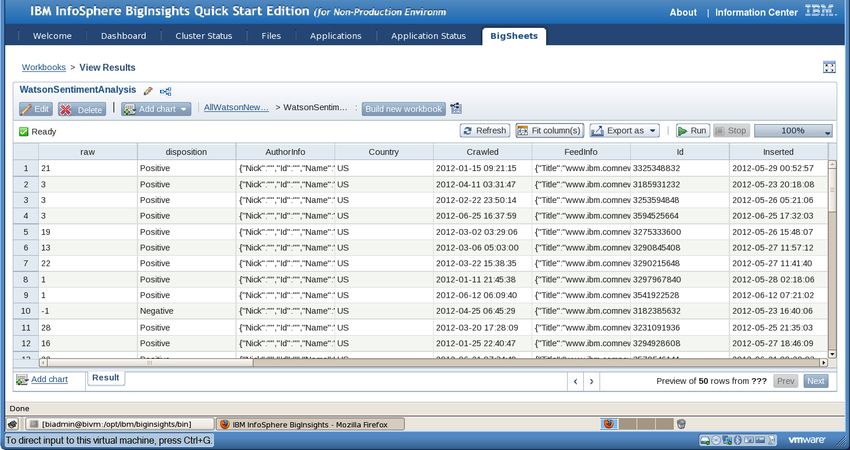
Table of Contents
Getting started with InfoSphere BigInsights .................................................................. 3


Exercise 1: BigInsights Web Console .............................................................................. 4

  Launching the Web Console ....................................................................................................................... 5

  Working with the Welcome page ................................................................................................................ 6

  Administering BigInsights .......................................................................................................................... 8

  Working with Files .................................................................................................................................... 11


Exercise 2: Social Media and BigSheets........................................................................ 16

  Collecting Social Media ........................................................................................................................... 17

  Creating a BigSheets Workbook ............................................................................................................... 20


Exercise 3: Querying data with IBM Big SQL ............................................................. 35

  Connecting to the IBM Big SQL server .................................................................................................... 36

  Creating a project and an SQL script file ................................................................................................ 38

  Creating tables and loading data ............................................................................................................. 40

  Running basic Big SQL queries ................................................................................................................ 42

  Analyzing the data with Big SQL .............................................................................................................. 45


Exercise 4: Developing, publishing, and deploying your first big data app .............. 49

  Developing your application .................................................................................................................... 49

  Publishing your application ..................................................................................................................... 50

  Deploy and run your application .............................................................................................................. 53


Exercise 5: Analyzing BigSheets data in IBM Big SQL .............................................. 56

  Create and modify a BigSheets workbook ................................................................................................ 57

  Export your Workbook .............................................................................................................................. 60

  Creating an Eclipse project and new SQL script ..................................................................................... 62

  Exporting a JSON Array to Big SQL ........................................................................................................ 68


Exercise 6: Text analysis of social media data............................................................. 70

  Upload and deploy the sample text analytics application ........................................................................ 71

  Upload sample data and create a master workbook ................................................................................ 73

  Analyzing text content of social media posts ............................................................................................ 77


Summary .......................................................................................................................... 83


                                                                              2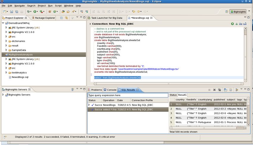
Getting started with InfoSphere BigInsights
In this hands-on lab, you'll learn how to work with IBM InfoSphere BigInsights to
analyze big data. In particular, you'll explore social media data using a spreadsheet-style
interface to discover insights about the global coverage of a popular brand without
writing any code. You'll also use Big SQL to query data managed by BigInsights and
learn how to develop, test, publish, and deploy your first big data application. Finally,
you'll see how business analysts can invoke a pre-packaged, custom text analytics
application that analyzes the sentiments expressed about a popular brand in news and
blog postings on the Web.

After completing this hands-on lab, you’ll be able to:

•       Navigate the BigInsights Web Console
•       Explore big data using a spreadsheet-style tool
•       Query big data using Big SQL
•       Create and run an application
•       Analyze text in social media data using a custom-built extractor

Allow 2.5 to 3 hours to complete the entire lab end-to-end.

This version of the lab was designed using the InfoSphere BigInsights 2.1 Quick Start
Edition. Throughout this lab, you will be using the following account login information:

                               Username                       Password
Linux                          biadmin                        biadmin

                                             3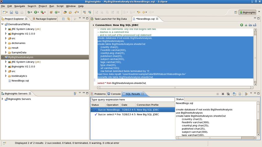
Exercise 1: BigInsights Web Console
IBM’s InfoSphere BigInsights 2.1 Enterprise Edition enables firms to store, process, and
analyze large volumes of various types of data. In this exercise, you’ll see how you can
work with its Web console to administer your system, launch applications (jobs), monitor
the status of applications, and perform other functions.

For further details on the Web console or BigInsights, visit the product's InfoCenter. In
addition, IBM's big data channel on YouTube contains a video demonstration of the Web
console.

After completing this hands-on lab, you’ll be able to:
   • Launch the Web console.
   • Work with popular resources accessible through the Welcome page.
   • Administer BigInsights by inspecting the status of your cluster, starting and
       stopping components, and accessing administrative tools available for open
       source components provided with BigInsights.
   • Work with the distributed file system. In particular, you'll explore the HDFS
       directory structure, create subdirectories, and upload files to HDFS.
   • Launch applications (jobs) and inspect their status.

Allow 30 minutes to complete this section of lab.

This lab is an introduction to a subset of console functions. Real-time monitoring
dashboards and application linking are among the more advanced console functions that
are out of this lab's scope.

                                            4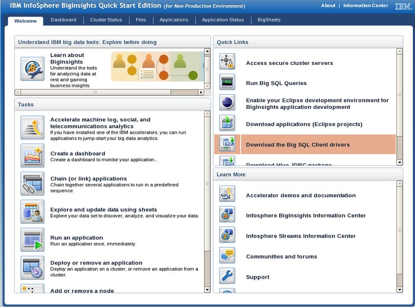
Launching the Web Console
The first step to accessing the BigInsights Web Console is to launch all of the BigInsights
processes (Hadoop, Hive, Oozie, Map/Reduce etc.). Once started, these services will
remain active for the remainder of this lab.

__1.    Select the Start BigInsights icon to start all services.

__2.    Select the BigInsights Console icon to launch the Web Console.

__3.    Verify that your Web console appears similar to this, and note each section:
        Tasks: Quick access to popular BigInsights tasks
        Quick Links: Links to internal and external quick links and downloads to
        enhance your environment
        Learn More: Online resources available to learn more about BigInsights

                                             5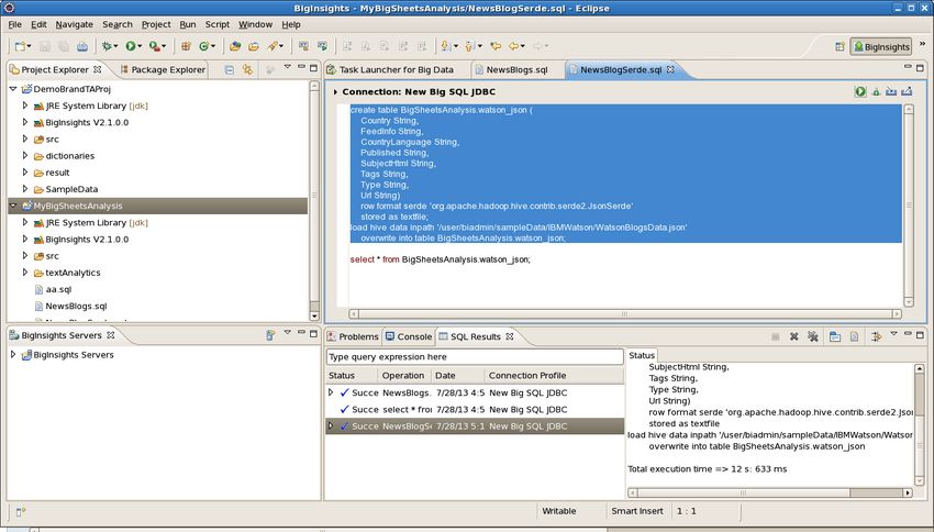
Working with the Welcome page
This section introduces you to the Web console's main page displayed through the
Welcome tab. The Welcome page features links to common tasks, many of which can
also be launched from other areas of the console. In addition, the Welcome page includes
links to popular external resources, such as the BigInsights InfoCenter (product
documentation) and community forum. You'll explore several aspects of this page.

__1.    In the Welcome Tab, the Tasks pane allows you to quickly access common
        tasks. Select the View, start or stop a service task. If necessary scroll down.

__2.    This takes you to the Cluster Status tab. Here, you can stop and start Hadoop
        services, as well as gain additional information as shown in the next section

__3.    Click on the Welcome tab to return back to the main page.

                                           6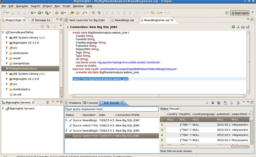
__4.   Inspect the Quick Links pane at top right and use its vertical scroll bar (if
       necessary) to become familiar with the various resources accessible through
       this pane. The first several links simply activate different tabs in the Web
       console, while subsequent links enable you to perform set-up functions, such as
       adding BigInsights plug-ins to your Eclipse development environment.

__5.   Inspect the Learn More pane at lower right. Links in this area access external
       Web resources that you may find useful, such as the Accelerator demos and
       documentation, BigInsights InfoCenter, a public discussion forum, IBM support,
       and IBM's BigInsights product site. If desired, click on one or more of these links
       to see what's available to you

                                           7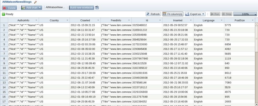
Administering BigInsights
The Web console allows administrators to inspect the overall health of the system as well
as perform basic functions, such as starting and stopping specific servers or components,
adding nodes to the cluster, and so on. You’ll explore a subset of these capabilities here.

Inspecting the status of your cluster

__1.    Click on the Cluster Status tab at the top of the page to return to the Cluster
        Status window

__2.    Inspect the overall status of your cluster. The figure below was taken on a
        single-node cluster that had several services running. One service – Monitoring
        -- was unavailable. (If you installed and started all BigInsights services on your
        cluster, your display will show all services as running.).

__3.    Click on the Hive service and note the detailed information provided for this
        service in the pane at right. From here, you can start or stop the hive service (or
        any service you select) depending on your needs. For example, you can see the
        URL for Hive's Web interface and its process ID.

                                             8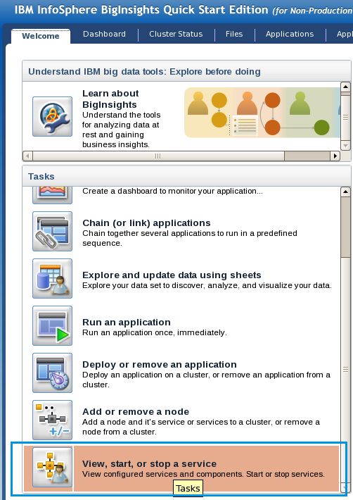
__4.   Optionally, cut-and-paste the URL for Hive’s Web interface into a new tab of
       your browser. You'll see an open source tool provided with Hive for
       administration purposes, as shown below.

__5.   Close this tab and return to the Cluster Status section of the BigInsights Web
       console
Starting and stopping a component

__6.   If necessary, click on the Hive service to display its status.

__7.   In the pane to the right (which displays the Hive status), click the red Stop button
       to stop the service

__8.   When prompted to confirm that you want to stop the Hive service, click OK and
       wait for the operation to complete. The right pane should appear similar to the
       following image

                                             9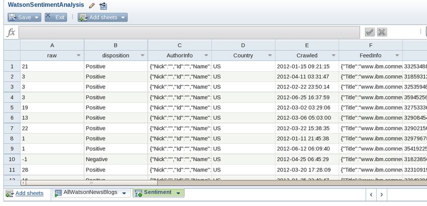
__9.    Restart the Hive service by clicking on the green arrow just beneath the Hive
        Status heading, as seen in the previous figure. When the operation completes
        (may take a minute), the Web console will indicate that Hive is running again,
        likely under a process ID that differs from the earlier Hive process ID shown at
        the beginning of this lab module. You may need to use the Refresh button of
        your Web browser to reload information displayed in the left pane.
Accessing service specific Web tools

__10.   Click on the Welcome tab

__11.   Click on the Access secure cluster servers button in the Quick Links section
        at right (ensure the pop-up blocker is disabled).

__12.   Inspect the list of server components for which there are additional Web-based
        tools. The BigInsights console displays the URLs you can use to access each of
        these Web sites directly. (Make sure your pop-up blocker is disabled for this
        step.)

__13.   Click on the namenode alias. Your browser will display the standard
        NameNode Web interface provided by Apache Hadoop, which is covered in a
        separate lab on HDFS and MapReduce.

                                           10
Working with Files
The Files tab of the console enables you to explore the contents of your file system,
create new subdirectories, upload small files for test purposes, and perform other file-
related functions. In this module, you’ll learn how to perform such tasks against the
Hadoop Distributed File System (HDFS) of BigInsights.
__1. Click on the Files tab of the Web console to begin exploring your distributed file
system.
__2. Expand the directory tree shown in the pane at left (/user/biadmin). If you
already uploaded files to HDFS, you’ll be able to navigate through the directory
to locate them.
11__3. Become familiar with the functions provided through the icons at the top of this
pane, as we'll refer to some of these in subsequent sections of this module.
Simply point your cursor at the icon to learn its function. From left to right, the
icons enable you to Copy a file or directory, move a file, create a directory,
rename a file or directory, upload a file to HDFS, download a file from HDFS to
your local file system, remove a file from HDFS, set permissions, open a
command window to launch HDFS shell commands, and refresh the Web
console page
__4. Position your cursor on the user/biadmin directory and click the Create
Directory icon to create a subdirectory for test purposes
__5. When a pop-up window appears prompting you for a directory name, enter
ConsoleLab and click OK
__6. Expand the directory hierarchy to verify that your new subdirectory was created.
12__7. Create another directory named ConsoleLabTest.
__8. Use the Rename icon to rename this directory to ConsoleLabTest2
__9. Click the Move icon, when the pop up Move screen appears select the
ConsoleLab directory and click OK.
13__10. Using the set permission icon, you can change the permission settings for your
directory. When finished click OK.
__11. While highlighting the ConsoleLabTest2 folder, select the Remove icon and
remove the directory.
14__12. Remain in the ConsoleLab directory, and click the Upload icon to upload a small
sample file for test purposes.
__13. When the pop-up window appears, click the Browse button to browse your local
file system for a sample file.
__14. Navigate through your local file system to the directory where BigInsights was
installed. For the IBM-provided VMware image, BigInsights is installed in file
system: /opt/ibm/biginsights. Locate the …/IHC subdirectory and select the
CHANGES.txt file. If you can’t find it, you may select a different file for this step.
Click OK
__15. Verify that the window displays the name of this file. Note that you can continue
to Browse for additional files to upload and that you can delete files as upload
targets from the displayed list. However, for this exercise, simply click OK
__16. When the upload completes, verify that the CHANGES.txt file appears in the
directory tree at left, if it is not immediately visible click the refresh button. On
the right, you should see a subset of the file’s contents displayed in text format
15__17. Highlight the CHANGES.txt file in your ConsoleLab directory and click the
Download button.
__18. When prompted, click the Save File button. Then select OK.
__19. If Firefox is set as default browser, the file will be saved to your user Downloads
directory. For this exercise, the default directory location is fine
Exercise 2: Social Media and BigSheets
IBM’s InfoSphere BigInsights 2.1 Enterprise Edition enables firms to store, process, and
analyze large volumes of various types of data. In this exercise, you’ll see how you can
find and ingest social media data from Boardreader and do some ad hoc data exploration
with BigSheets. This lab is based on an article that can be found here:
16http://www.ibm.com/developerworks/data/library/techarticle/dm-
1206socialmedia/index.html
If you have not done so, it is suggested that you read the article before attempting this lab
as additional details are contained in the article that will help you understand the business
reasons for taking the actions we take in the following lab steps. You can also watch a
14-minute video from the author of the article here:
http://www.youtube.com/watch?v=kny3nPwSZ_w
After completing this hands-on lab, you’ll be able to:
• Create a Big Sheets workbook in order to process some of the Boardreader input
data that has been loaded into the HDFS for you.
• Create Big Sheets visualizations to see some of the quantitative analytics.
Allow 45 minutes to complete this lab.
Where did this data come from?
For time efficiency of this lab, the data was already
collected using the BoardReader application. BoardReader
was used to collect data from news and blog websites, with
the output saved into your HDFS.
Collecting Social Media
__1. If your BigInsights services aren’t started, select the Start BigInsights icon.
17__2. Launch the BigInsights WebConsole icon to launch the Web Console
__3. Verify that your Web console appears similar to this:
The social media output that will be used for this lab has been preloaded into the HDFS.
This data was retrieved using the Boardreader app. To learn how to use the Boardreader
app to pull social media data, refer to the BigSheets developerWorks article referenced
above.
__4. To review this data, use the Files tab to navigate to the following folder
(/user/biadmin/sampleData/IBMWatson) and select the blogs-data.txt file as
shown below
18__5. In a future section, we will display this text file within BigSheets in order to
display, interact with, and visualize the data within BigInsights.
19Creating a BigSheets Workbook
In this section, we will use the spreadsheet style interface known as BigSheets.
BigSheets provides access to data in items known as “workbooks.”
Creating a Workbook from Boardreader Data
__1. Return to the Files tab.
__2. Navigate to the /user/biadmin/sampleData/IBMWatson/blogs-data.txt file. Make
sure this file is selected.
__3. Click the Sheet radio button to view this data within a BigSheets interface.
__4. The data that comes from the Boardreader application within BigInsights is
formatted in a JSON Array structure. You will need to click on the pencil icon
and select the JSON Array option for this file. Then click the green check.
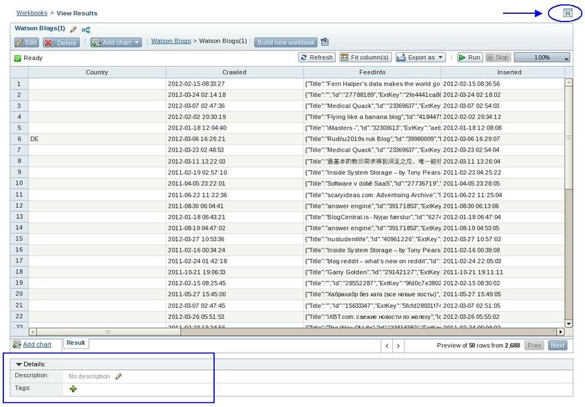
20__5. Save this as a Master Workbook named “Watson Blogs”. You can optionally
provide a description. Click the Save button.
__6. You will want to do the same thing for the news-data.txt file in the same folder.
To do this, you will need to return to the Files tab, navigate to the file, and follow
the same process. This time, you will provide the name “Watson News”.
__7. Click on the “Workbooks” link in the upper left-hand corner of the page.
__8. You should now see (2) or more workbooks on your system, depending on the
configuration of your VM. The top (2) are the ones you created in the previous
steps.
__9. Adding tags allows us to quickly search and manage workbooks. Select the
“Watson Blogs” workbook.
__10. Scroll down to Workbook Details, add the following tags “Watson” “IBM”
“Blogs” by selecting the green + and adding each individually. If you don’t see
Workbook Details, you may need to toggle between Normal and Full Screen.
21__11. From the BigSheets tab, you can quickly filter workbooks and search for a
specific tag. Enter the term “tag: Blogs” to see all workbooks that have the
associated tag.
22Tailoring Your Workbooks
In this section, we will first show you how to reduce the amount of data you are working
with by removing unwanted columns from within your BigSheets Workbooks. We will
also perform a merge or “union” of two data workbooks.
__12. From the list of Workbooks (you launched in the previous steps), click on the link
named “Watson News” to open this workbook in BigSheets.
__13. This Master Workbook is a “base” workbook and has a limited set of things you
can edit. Therefore, in order to begin to manipulate the data contained within a
workbook, we will want to create a dependent workbook.
__a. Click the “Build new Workbook” button
__b. When the new Workbook appears, you can change its default name (by
clicking on the pencil icon next to the name) to the new name of
“Watson News Revised” then click the green check mark.
__c. Click the Fit column(s) button to more easily see columns A through H
on your screen
.
23__14. You have decided you would like to remove the column “IsAdult” from your
workbook. This is currently column E. Click on the triangle next to the column
name of “IsAdult” and select the “Remove” option to remove this from your new
workbook.
Did I lose data?
Deleting a column does not remove data. Deleting a
column in a workbook just removing the mapping to this
column.
__15. In this case, you want to keep only a few columns. In order, to more easily
remove a larger number of columns (without having to do this same click-
remove process), click the triangle again (from any column) and select the
“Organize Columns…” option.
__a. Click the red X button next to each column title you want to remove.
In this case, KEEP the following columns…
__i. Country
__ii. FeedInfo
__iii. Language
__iv. Published
__v. SubjectHtml
__vi. Tags
__vii. Type
__viii. Url
24__b. Click the green check mark button when you are ready to remove the
columns you have selected to remove.
__16. Click on the Fit column(s) button again to show columns A through H. You
should see the following columns in your new workbook.
__17. Select “Save and Exit”. You may input an optional description. Click Save to
complete the save.
__18. After clicking Save, you will be shown two buttons (run and close). Click the
Run button to run the workbook. You can monitor the progress of your request
by watching the status bar indicator in the upper right-hand side of the page.
__19. To reduce the unwanted columns in the “Watson Blogs” workbook, you will
want to perform the same steps above in order to wind up with a new workbook
called “Watson Blogs Revised”
25__20. Now, since we have two workbooks with the exact same structure, we can
perform a “union” of these two workbooks as the basis for exploring the
coverage of IBM Watson across the sources that Boardreader provided.
__21. To perform this action, make sure you are currently in the “Watson News
Revised” workbook. Click the “Build New Workbook” button again.
__22. In the top left-hand side or bottom left, you should see a link called “Add
sheets”. This allows you to perform additional analysis on your data within the
current workbook. Click the “Add sheets” link.
__23. The Load option will allow you to load data into the current workbook from
another workbook. Click the Load icon and select the “Watson Blogs Revised”
workbook link.
__24. The system will ask you for a *Sheet Name and you should change Sheet1 to
“Watson Blogs Revised” as the name of the new tab that will be created in
your current workbook.
26__25. Click the green check-mark button at this time to load the new workbook into
your current workbook.
__26. You should now see two tabs at the bottom on your current workbook. If you
move your mouse over the second one, a tooltip will show the action and the
name you provided for this sheet / tab within you current workbook. (Giving your
tabs meaningful names will help you and other that use your sheets an easy
way to understand your data processing flow(s).)
__27. Next, we need to add a new sheet to perform the Union function. Select Union.
__28. The Union function asked for the other “sheet” you would like to use. Select the
triangle to expose the pull-down menu.
__29. Select ”Watson News Revised” and then click the green plus-mark button.
__30. Then provide the sheet name “News and Blogs”. Before you click the green
check-mark button to add this new tab/sheet to your workbook, make sure your
options match the example below.
27__31. Click the green check-mark button to add this tab to your workbook.
__32. Save and Exit and then run this new workbook. When prompted for a
description, you can change the name of your new workbook from “Watson
News Revised(1)” to “Watson News and Blogs”. Click the Save button. Then
click the Run button to run the workbook.
__33. Select the Workflow Diagram icon to see a mapping of the workbooks
associated with the News and Blogs workbook. This can be done at any point to
keep a clear picture of which workbooks you are extending to/from.
__34. Close this frame and you can continue to the next section.
Exploring Your Workbook
In this section, we will explore the data in your new workbook. You will perform actions
like sorting, charting, cleansing, and grouping to make analysis of the HDFS data easier
via BigSheets.
__35. If you are not already in the workbook, open the “Watson News and Blogs”
workbook.
__36. In this case, we want to keep our initial workbook “as is” and produce another
workbook that contains the records in sorted order. So, click the “Build New
Workbook” button to do this.
__37. As a way to keep track of what you are doing, I typically suggest that you
rename your new workbook right away as this helps to remind you of what you
are working on. So, provide a new name for your workbook, like “Watson
Sorted”.
28__38. After looking at the data, you decide you would like to understand more about
the language and the types of posts contained in your workbook.
__39. Clicking on the triangle next to the column name of any column, you will want to
click on the Sort -> Advanced option
.
__40. Then, you will click on the pull-down triangle to expose the list of columns under
the “Add Columns to Sort” area. Click on the green + button to add the two
columns you wish to sort on. Then, select the desired order for sorting each
column. In this case, your “Advance Sort” should look like the following picture.
__41. Click on the green check-mark button to continue and create the new tab/sheet
with your desired sorting applied to it.
__42. As with all new tabs/sheets, the system shows you a simulated result based on
the rows of data BigSheets keeps in memory. You should be able to click on Fit
column(s) to review the contents of both the Language and Type columns to
see that your “advanced sort” was applied to this simulated set of data.
29__43. Now, “Save and Exit” and then run your workbook. This will apply the sorting
options to more than the first 2,000 rows the system operates on as a
simulation. This will sort the entire, larger data in the workbook. So, you should
see different results once your workbook has been run. For example, in the
simulated data, only one Vietnamese row was showing. However, against the
entire data set, you should see twenty (20) rows that are of the Vietnamese
language. This is because more of the Vietnamese rows were in the data
beyond the first 2,000 rows the system uses in memory for a simulated result
before you click the run button. Review and confirm these results after the job
reaches 100% and then you can move onto the next step.
__44. To visualize this data better, you want to analyze the quantities of posts in the
various languages in your current workbook. While still in the “Watson Sorted”
workbook.
__45. Click on the “Add chart” link in the lower left (this may take a minute to populate
the chart types the first time it is run), click on chart, then pie, and fill out the
following information to produce a pie chart of the languages used.
__46. Click on the green check-mark button to create the chart tab.
__47. Just like working with tabular data, you will see a simulated visualization. Again,
this is based on the rows in cache. (If you click on the Close button here, you
can interact with the chart which is based on simulated data. You would then
click the “Run” button in the upper right.)
30__48. Click the Run button to run the visualization against the entire data set.
__49. Once the chart has been run, you can interact with it to find out the second,
most-popular language for posts regarding IBM Watson is Russian. Move your
mouse over this item within your pie chart to see these results.
__50. Additionally, you have decided you need to clean up some of the data within the
workbook. Based on the fifth and sixth largest languages in the pie chart you
just generated, you can see they are both variations on the Chinese language.
__51. Let’s perform an action to clean up this data which will show all Chinese items in
the same bucket. To do this, we will combine these two items into one item
called Chinese
31__52. From the “Watson Sorted” workbook, you will want to click on the edit button in
order to go back into edit mode for this workbook.
__53. To make things easier, you can optionally click on the Fit column(s) button to
make your columns thinner and to see more data on the screen.
__54. At this point, you have decided to add another column to your workbook. To do
this, click on the triangle next to the Language column name. Select the Insert
Right -> New Column option.
__55. Then, you will provide a name for your new column, like “Language_Revised”
and then click the green check-mark button (or hit enter) to apply your new
column name.
__56. Your cursor is then moved to the fx (or function) area where you can provide the
function to be used to generate the contents of your new column.
__57. Enter the following formula as your function…
IF(SEARCH('Chin*', #Language) > 0, 'Chinese', #Language)
32This formula looks at the Language column indicated by #Language. If the #Language
column starts with ‘Chin*’, then the new #Language_Revised column with contain
‘Chinese’. If it does not, the value of #Language is copied over to #Language_Revised.
(See the original article, URL at the top of this document, for additional explanation of
this formula.)
__58. Clicking on the green check-mark button (or hitting enter) should produce
content in your new column based on your new formula.
__59. “Save and Exit” and you should notice that you receive a message to “Click
run to update the data”
__60. Click the Run button in the upper right to run the workbook.
__61. Now, click on the Language Coverage tab that contains your previously
generated pie chart. This now has the status of “needs to be run”. Before we
run it, we need to change one of the settings on the pie chart to use our newly
generated column named Language_Revised.
__62. To change the settings, click on the triangle next to the Language Coverage tab.
__63. Click to select the “Chart Settings” option.
__64. Change the “Value:” item to be based on the new, Language_Revised column.
33__65. Click on the green check-mark button to apply your new settings.
__66. Click on the Run button to regenerate your pie chart.
__67. Once your new pie chart has been generated, you should be able to see
Chinese as a cleaned up, single item in your pie chart (compared to the two
items you saw previously). With this cleansed data, Chinese is now the second
largest and Russian is third.
34Exercise 3: Querying data with IBM Big SQL
Learn how to use IBM Big SQL, an SQL language processor, to summarize, query, and
analyze data in a data warehouse system for Hadoop. Big SQL provides broad SQL
support that is typical of commercial databases. You can issue queries using JDBC or
ODBC drivers to access data that is stored in InfoSphere BigInsights, in the same way
that you access databases from your enterprise applications. You can use the Big SQL
server to execute standard SQL queries. Multiple queries can be executed concurrently.
Big SQL provides support for large ad hoc queries by using MapReduce parallelism and
point queries, which are low-latency queries that return information quickly to reduce
response time and provide improved access to data. The Big SQL server is multi-
threaded, so scalability is limited only by the performance and number of CPUs on the
computer that runs the server. If you want to issue larger queries, you can increase the
hardware performance of the server computer that Big SQL runs on.
This tutorial uses data from the fictional Sample Outdoor Company. The Sample
Outdoor Company sells and distributes outdoor products to third-party retailer stores
around the world. The company also sells directly to consumers through its online store.
For the last several years, the company has steadily grown into a worldwide operation,
selling their line of products to retailers in nearly every part of the world.
The fictional Sample Outdoor Company began as a business-to-business operation. The
company does not manufacture its own products; rather, the products are manufactured
by a third party, then the products are sold to third-party retailers. The company is
expanding its business by creating a presence on the web. Now they also sell directly to
consumers through their online store. You will learn more about the products and sales of
the fictional Sample Outdoor Company by running Big SQL queries and doing the
analysis on the data in the following lessons.
35In this lab, you will use the InfoSphere BigInsights Tools for Eclipse to create Big SQL
queries so that you can extract large subsets of data for analysis.
After you complete the lessons in this module, you will understand the concepts and
know how to do the following actions:
• Connect to the Big SQL server by using the InfoSphere BigInsights Tools for
Eclipse. Use the InfoSphere BigInsights Tools for Eclipse to load sample data and
to create queries.
• Use BigSheets to analyze data generated from Big SQL queries.
• Use the InfoSphere BigInsights Console to run Big SQL queries.
• Use the InfoSphere BigInsights Tools for Eclipse to export data.
This module should take approximately 45 minutes to complete.
Connecting to the IBM Big SQL server
In this section, you view the JDBC connection, learn how to navigate to the Data
Management view in Eclipse, and how to open the SQL editor. Big SQL is installed with
the InfoSphere BigInsights in the following directory: $BIGSQL_HOME/bin/bigsql.
Ensure that you complete the following actions before you begin the tutorial:
__1. Review the status of Big SQL. From the InfoSphere BigInsights Console, click
the Cluster Status page. Then, verify that the Big SQL node is in a Running
state on the Big SQL Server Summary page. If it is not started, click on Start in
the Big SQL Server Summary page.
__2. Start Eclipse and select the default workspace.
36If you created an InfoSphere BigInsights server connection to a particular BigInsights
server, the Big SQL JDBC driver connection and the Big SQL JDBC connection profile
were both created for you automatically. Ensure that a JDBC driver definition exists.
Generally, either a JDBC or an ODBC driver definition must exist before you can create
a connection to a Big SQL server. For the purposes of this tutorial, only a JDBC driver
definition is required.
__3. From the Eclipse environment, click Window > Open Perspective > Other >
Database Development. Ensure that the Data Source Explorer view is open.
__4. From the Data Source Explorer view, expand the Database Connections folder.
__5. Right-click the Big SQL connection, select Properties. Verify the connection
details.
__6. Click Test Connection to make sure that you have a valid connection to the Big
SQL server. If the ping succeeded, you may skip to the next section.
If you do not have a connection, follow these steps:
__a. From the Data Source Explorer view, right-click the Database
Connections directory and click Add Repository.
37__b. In the New Connection Profile window, select Big SQL JDBC in the
Connection Profile Types list. Edit the text in the Name field or the
Description field, and click Next.
__c. In the Specify a Driver and Connection Details window, select IBM Big
SQL JDBC Driver Default from the Drivers list. You can add or modify a
driver by clicking the New Driver Definition icon or the Edit Driver
Definition icon.
__d. The Connection URL field displays the URL that is generated. For
example: jdbc:bigsql://bivm:7052/default
__e. Specify the Connect when the wizard completes check box to connect to
the Big SQL server after you finish defining this connection profile.
__f. Specify the Connect every time the workbench is started to connect to
the Big SQL server automatically by using this connection profile when
you launch this Eclipse workspace.
__g. Click Test Connection to verify that the connection. Click Finish to save.
Creating a project and an SQL script file
You can create Big SQL scripts and run them from the InfoSphere BigInsights
Eclipse environment.
__1. Create an InfoSphere BigInsights project in Eclipse. From the Eclipse menu bar,
click File > New > Other. Expand the BigInsights folder, select BigInsights
Project, and then click Next.
__2. Type myBigSQL in the Project name field, and then click Finish.
__3. If you are not already in the BigInsights perspective, a Switch to the BigInsights
perspective window opens. Click Yes to switch to the BigInsights perspective.
__4. Create an SQL script file. From the Eclipse menu bar, click File > New > Other.
Expand the BigInsights folder, and select SQL Script, and then click Next.
__5. In the New SQL File window, in the Enter or select the parent folder field, select
myBigSQL. Your new SQL file is stored in this project folder.
38__6. In the File name field, type aFirstFile. The .sql file extension is added
automatically. Click Finish.
__7. In the Select Connection Profile window, select the Big SQL connection. The
properties of the selected connection display in the Properties field. When you
select the Big SQL connection, the Big SQL database-specific context assistant
and syntax checks are activated in the editor that is used to edit your SQL file.
__8. Click Finish to close the Select Connection Profile window.
__9. In the SQL Editor that opens the aFirstFile.sql SQL file you created, add the
following Big SQL comments:
39-- This is a beginning SQL script
-- These are comments. Any line that begins with two
-- dashes is a comment line,
-- and is not part of the processed SQL statements.
Some lines in the file contain two dashes in front of text. Those dashes mark the text as
comment lines. Comment lines are not part of the processed code. It is always useful to
comment your Big SQL code as you write the code, so that the reasons for using some
statements are clear to all who must use the file. You will be using this file in later
lessons.
__10. Save aFirstFile.sql by using the keyboard short, CTRL-S.
Creating tables and loading data
In this lesson, you will create the tables, and load the data that you will use to run queries
and create reports about the fictional Sample Outdoor Company. The examples in this
tutorial use Big SQL tables and data that are managed by Hive.
This tutorial uses sample data that is provided in the $BIGSQL_HOME/samples folder on
the local file system of the InfoSphere BigInsights server. By default, the
$BIGSQL_HOME environment variable is set to the installed location, which is
/opt/ibm/biginsights/bigsql/.
The time range of the fictional Sample Outdoor Company data is 3 years and 7 months,
starting January 1, 2004 and ending July 31, 2007. The 43-month period reflects the
history that is made available for analysis.
The schema that is used in this tutorial is the GOSALESDW. It contains fact tables for
the following areas:
• Distribution
• Finance
• Geography
• Marketing
• Organization
• Personnel
• Products
• Retailers
• Sales
• Time.
Access the sample SQL files
40__1. Open a Terminal. It is located in the desktop folder BigInsights Shell.
__2. Change your directory to $BIGSQL_HOME/samples. Open and review the
information in the README file.
__3. Open a new Terminal and type the setup command:
./setup.sh -u biadmin -p biadmin
__4. The script runs when you see this message:
Loading the data .. will take a few minutes to complete ..
Please check
/var/ibm/biginsights/bigsql/temp/GOSALESDW_LOAD.OUT file
for progress information.
The script runs three files: GOSALESDW_drop.sql, GOSALESDW_ddl.sql, and
GOSALESDW_load.sql.
__5. You can see the tables in the InfoSphere BigInsights Console Files tab:
hdfs://biginsights/hive/warehouse/gosalesdw.db
41Running basic Big SQL queries
You now have tables with data that represents the fictional Sample Outdoor Company. In
this lesson, you will explore some of the basic Big SQL queries, and begin to understand
the sample data.
You will use the SQL file that you created earlier to test the tables and data that you
created in the previous lesson. In this lesson, several sample SQL files that are included
with the downloaded Big SQL samples can be used to examine the data, and to learn how
to manipulate Big SQL.
__1. From the Eclipse Project Explorer, open the myBigSQL project, and double-click
the aFirstFile.sql file.
__2. In the SQL editor pane, type the following statement:
SELECT * FROM GOSALESDW.GO_REGION_DIM;
Each complete SQL statement must end with a semi-colon. The statement selects, or
fetches, all the rows that exist in the GO_REGION_DIM table.
__3. Click the Run SQL icon.
42Depending on how much data is in the table, a SELECT * statement might take some
time to complete. Your result should contain 21 records or rows.
You might have a script that contains several queries. When you want to run the entire
script, click the Run SQL icon. When you want to run a specific statement, or set of
statements, and you include the schema name with the table name
(gosalesdw.go_region_dim), highlight the statement or statements that you want to run
and press F5.
__4. Improve the SELECT * statement by adding a predicate to the second statement
to return fewer rows. A predicate is a condition on a query that reduces and
narrows the focus of the result. A predicate on a query with a multi-way join can
improve the performance of the query.
SELECT * FROM GOSALESDW.GO_REGION_DIM WHERE REGION_EN LIKE
'Amer%';
__5. Click Run SQL to run the entire script. This query results in four records or rows.
It might run more efficiently than the original statement because of the predicate.
Tip: If you get an error, type out the full query instead of using copy/paste.
__6. You can learn something more about the structure of the table with some
queries to the syscat table. The Big SQL catalog tables provide metadata
support to the database. The Big SQL catalog consists of four tables in the
schema SYSCAT: schemas, tables, columns, and index columns. Type the
following query, and this time, select the statement, and press F5.
SELECT * FROM syscat.columns
43WHERE tablename=
'go_region_dim'
AND schemaname=
'gosalesdw';
This query uses two predicates in a WHERE clause. The query finds all of the
information from the syscat.columns table as long as the tablename is 'go_region_dim'
and the schemaname is 'gosalesdw'. Since you are using AND, both predicates must be
true to return a row. Use single quotation marks around string values.
The result of the query to the syscat.columns table is the metadata, or the structure of the
table. Look at the SQL Results tab in Eclipse to see your output. The SQL Results tab in
Eclipse shows 54 rows as your output. That means that there are 54 columns in the table
go_region_dim.
__7. In addition to the query to learn about the structure of a table, you can also run a
query that returns the number of rows in a table. Type the following query, select
the statement, and then press F5.
SELECT COUNT(*) FROM gosalesdw.go_region_dim;
The COUNT aggregate function returns the number of rows in the table, or the number of
rows that satisfy the WHERE clause in the SELECT statement, if a WHERE clause was
part of the statement. The result is the number of rows in the set. A row that includes only
null values is included in the count. In this example, there are 21 rows in the
go_region_dim table.
__8. Another form of the count function is the COUNT (distinct )
statement. As the name implies, you can determine the number of unique values
in a column, such as region_en. Type this statement in your SQL file:
SELECT COUNT (distinct region_en) FROM gosalesdw.go_region_dim;
44The result is 5. This result means that there are five unique region names in English (the
column name region_en).
__9. Another useful statement in Big SQL is the LIMIT clause. The LIMIT clause
specifies a limit on the number of output rows that are produced by the SELECT
statement for a given document. Type this statement in your SQL file, select the
statement, and then press F5:
SELECT * FROM GOSALESDW.DIST_INVENTORY_FACT limit 50;
The statement returns 53837 rows without the limit clause and depending on the setting
in the Eclipse preferences for the SQL Results View. If there are fewer rows than the
LIMIT value, then all of the rows are returned. This statement is useful to see some
output quickly.
__10. Save your SQL file.
Analyzing the data with Big SQL
In this lesson, you create and run Big SQL queries so that you can better understand the
products and market trends of the fictional Sample Outdoor Company.
__1. Create an SQL file. From the Eclipse menu, click File > New > Other. In the
Select a wizard window, expand the BigInsights folder, select SQL Script from
the list of wizards, and then click Next. In the New SQL File window, select the
myBigSQL project folder in the Enter or select the parent folder field. In the File
name field, type companyInfo. The .sql file extension is added automatically.
Click Finish.
To learn what products were ordered from the fictional Sample Outdoor Company, and
by what method they were ordered, you must join information from multiple tables in the
45gosalesdw database because it is a relational database where not everything is in one
table.
__2. Type the following comments and statement into the companyInfo.sql file:
-- Fetch the product name and the quantity and
-- the order method.
-- Product name has a key that is part of other
-- tables that we can use as a join predicate.
-- The order method has a key that we can use
-- as another join predicate.
-- Query 1
SELECT pnumb.product_name, sales.quantity,
meth.order_method_en
FROM
gosalesdw.sls_sales_fact sales,
gosalesdw.sls_product_dim prod,
gosalesdw.sls_product_lookup pnumb,
gosalesdw.sls_order_method_dim meth
WHERE
pnumb.product_language='EN'
AND sales.product_key=prod.product_key
AND prod.product_number=pnumb.product_number
AND meth.order_method_key=sales.order_method_key;
Because there is more than one table reference in the FROM clause, the query can join
rows from those tables. A join predicate specifies a relationship between at least one
column from each table to be joined.
• The predicates such as prod.product_number=pnumb.product_number help to
narrow the results to product numbers that match in two tables.
• This query also uses an alias in the SELECT and FROM clauses, such as
pnumb.product_name. pnumb is the alias for the gosalesdw.sls_product_lookup
table. That alias can now be used in the where clause so that you do not need to
repeat the complete table name, and the WHERE clause is not ambiguous.
• The use of the predicate and pnumb.product_language=’EN’ helps to further
narrow the result to only English output. This database contains thousands of
rows of data in various languages, so restricting the language provides some
optimization.
46__3. Highlight the statement, beginning with the keyword SELECT and ending with
the semi-colon, and press F5. Review the results in the SQL Results page. You
can now begin to see what products are sold, and how they are ordered by
customers.
__4. By default, the Eclipse SQL Results page limits the output to only 500 rows. You
can change that value in the Data Management preferences. However, to find
out how many rows the query actually returns in a full Big SQL environment,
type the following query into the companyInfo.sql file, then select the query, and
then press F5:
--Query 2
SELECT COUNT(*)
--(SELECT pnumb.product_name, sales.quantity,
-- meth.order_method_en
FROM
gosalesdw.sls_sales_fact sales,
gosalesdw.sls_product_dim prod,
gosalesdw.sls_product_lookup pnumb,
gosalesdw.sls_order_method_dim meth
WHERE
pnumb.product_language='EN'
AND sales.product_key=prod.product_key
AND prod.product_number=pnumb.product_number
AND meth.order_method_key=sales.order_method_key;
47The result for the query is 446,023 rows.
__5. Update the query that is labeled --Query 1 to restrict the order method to equal
only 'Sales visit'. Add the following string just before the semi-colon:
AND order_method_en='Sales
visit'
__6. Select the entire --Query 1 statement, and press F5. The result of the query
displays in the SQL Results page in Eclipse.
The results now show the product and the quantity that is ordered by customers actually
visiting a retail shop.
48__7. To find out which method of all the methods has the greatest quantity of orders,
you must add a GROUP BY clause (group by pll.product_line_en,
md.order_method_en). You will also use a SUM aggregate function
(sum(sf.quantity)) to total the orders by product and method. In addition, you can
clean up the output a bit by using an alias (as Product) to substitute a more
readable column header.
-- Query 3
SELECT pll.product_line_en AS Product,
md.order_method_en AS Order_method,
sum(sf.QUANTITY) AS total
FROM gosalesdw.sls_order_method_dim AS md,
gosalesdw.sls_product_dim AS pd,
gosalesdw.sls_product_line_lookup AS pll,
gosalesdw.sls_product_brand_lookup AS pbl,
gosalesdw.sls_sales_fact AS sf
WHERE
pd.product_key = sf.product_key
AND md.order_method_key = sf.order_method_key
AND pll.product_line_code = pd.product_line_code
AND pbl.product_brand_code = pd.product_brand_code
GROUP BY pll.product_line_en, md.order_method_en;
__8. Select the complete statement, and press F5.
Your results in the SQL Results page show 35 rows.
Exercise 4: Developing, publishing, and deploying your
first big data app
In this lesson, you will learn how to publish an application that can run a simple Big SQL
script. After you create scripts that contain Big SQL statements or commands, you can
create applications that can run those Big SQL scripts with or without variables.
For the purposes of this lesson, you are going to create a new project that contains one
simple Big SQL script.
Developing your application
__1. Create a project to hold the script and the application information. In the Eclipse
Project Explorer, click File > New > BigInsights Project. In the New BigInsights
Project window, type MyTestApp in the Project name field. Click Finish.
__2. Verify that the sample data (IOD_sampleData/RDBMS_data.csv) is located on
your desktop folder called biadmin’s Home
49Create a Big SQL script within the MyTestApp project that creates a table if it does not
already exist, and then loads data into the table from a local file.
__3. Right-click the MyTestApp project and select New > SQL Script. In the File
name field, type LoadLocal.sql, select BigSQL connection. Click Finish.
__4. Type or copy the following code into the LoadLocal.sql file:
create table if not exists media_csv
(id integer not null,
name varchar(50),
url varchar(50),
contactdate string)
row format delimited
fields terminated by ','
stored as textfile;
load hive data local inpath
'/home/biadmin/IOD_sampleData/RDBMS_data.csv'
-- overwrite
into table media_csv;
Be sure to modify the inpath parameter value to match the path where you extracted the
files.
__5. Save the LoadLocal.sql file.
Publishing your application
__1. In the Eclipse Project Explorer, right-click the MyTestApp project, and select
BigInsights Application Publish.
50From the BigInsights Application Publish window, complete the wizard with the
following information:
__2. Location page - Verify the server name and click Next. If you do not have a valid
connection to a Big SQL server, you can create one by clicking Create.
__3. Application page - Specify to Create New Application.
__a. Type an application name in the Name field, such as myBigSQLApp.
51__b. You can type some text in the Description field. This text is optional, but
can help others to understand how to run your application when it is
deployed on the server.
__c. Optionally, select an icon that contains a visual identifier for this
application file from the local file path by clicking Browse. You can use a
default icon that is provided by the server.
__d. List one or more categories, such as load, that you want the application
to be listed under. This category is a helpful tag when you search for
new applications to deploy.
__e. Click Next.
__4. Type page - Select Workflow as the Application Type, and click Next.
__5. Workflow page
__a. Specify to Create a new single action workflow.xml file
__b. Select Big SQL from the Action Type drop down list.
__c. In the Properties pane, list the properties that you need.
52__i. Specify the name of the script that contains your Big SQL
statements so that you can run that script from the InfoSphere
BigInsights server. Select script from the list. Enter
“LoadLocal.sql” in the Value field. The Variable field is false.
Specify the credentials properties file for connecting to Big SQL.
__ii. Click New.
__iii. In the New Property window, in the Name field, select the
property credentials_prop from the list.
__iv. In the Value field, specify the name of your properties file in the
BigInsights credentials store. Type /user/biadmin/
credstore/private/bigsql.properties
__d. Parameters page - If you have parameters that you want to add, click
New. In this case, click Next. Note: The simple script that you are using
in this lesson does not need parameters.
__6. Publish page - You see the structure of your application in the preview of the
BIApp.zip file. You can click Add to add other scripts or supporting information.
Click Finish.
Deploy and run your application
53The application that you just published from Eclipse is now in the InfoSphere BigInsights
Console.
__1. Click the Application tab of the InfoSphere BigInsights Console, and click
Manage to see the new application.
__2. Find the myBigSQLApp application by the application title.
__3. Highlight the application and click Deploy.
__4. In the Deploy Application window, click Deploy.
__5. Click Run in the Applications tab. You see the myBigSQLApp in the list of
deployed applications. Double-click the application.
54__6. In the application, type some name in the Execution Name field, such as Test1
to identify a particular run time instance. Since everything in this application was
hardcoded, you can now click Run.
__7. If the application runs successfully, you see a green checked box. If the
application failed, you see a red box. You can examine the log by selecting the
arrow in the Details column of the Application History pane.
Examine the output of your application:
__8. Click on the Files tab of the InfoSphere BigInsights Console. Navigate to the
directory of the Hive warehouse (such as /biginsights/hive/warehouse).
__9. You can see that a new folder that represents the media_csv table is created.
Expand the folder to see the RDBMS_data.csv file.
__10. Click the file to display its contents.
__11. You can also issue a select statement from your Eclipse project, or from the Big
SQL Console of InfoSphere BigInsights to see the contents in Big SQL:
Select * from media_csv;
You have created an application that creates a table with columns, if that table does not
already exist. The application then loads data into the table from a local file. If you run
the application again, it loads a duplicate set of the data. You can fill the file with new
data, and run the application again, and it loads that new data.
You can quickly see that this kind of exercise can be useful if you need to see refreshed
data regularly. By adding scheduling information onto the application, you can have the
application run daily or weekly to add or refresh the data. By including variables into the
application, you can run the application with data from your dynamic input. You can
uncomment the overwrite clause to add new data for each application run.
55You can also read