Waves EARTHQUAKE DATA ANALYSIS, LOCATION & MAGNITUDE CALCULATION - T:+61 3 8420 8940 - ESS Earth Sciences
←
→
Page content transcription
If your browser does not render page correctly, please read the page content below
Waves
EARTHQUAKE DATA ANALYSIS, LOCATION & MAGNITUDE CALCULATION

141 Palmer Street, Richmond VIC 3121 Australia   T:+61 3 8420 8940   sales@src.com.au
Version 4.2
    23 August 2021
        Author: AP

2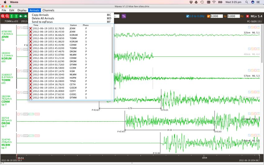
Table of Contents
History ....................................................................................................... 5
  The Seismology Research Centre ............................................................................ 5
  Data Formats ....................................................................................................... 5
Installing Waves ........................................................................................ 6
     Java Not Required ........................................................................................................... 6
     Waves Workspace ........................................................................................................... 6
Toolbar & Channel Buttons ......................................................................... 7
Controls ..................................................................................................... 8
  Zooming & Scrolling .............................................................................................. 8
     Scroll-zoom .................................................................................................................... 8
     Click-zoom ..................................................................................................................... 8
     Swipe-zoom ................................................................................................................... 8
     Timeline scrolling ............................................................................................................ 8
     Amplitude scaling ............................................................................................................ 8
  Picking Arrivals ..................................................................................................... 9
  Amplitude Grouping .............................................................................................. 9
  Zero Correction ................................................................................................... 10
  Trim ................................................................................................................... 10
  Vector Sum ......................................................................................................... 11
  Using the “Sync” feature ....................................................................................... 11
  File Filter ............................................................................................................ 12
  Frequency Filters ................................................................................................. 12
Waveform Display Elements ..................................................................... 13
  Decoding the Y-axis Labels .................................................................................... 14
  Display of Ground Motion Units .............................................................................. 14
  Minimise and Maximise Channels ........................................................................... 14
  Channel Rotation ................................................................................................. 15
  Channel Polarity .................................................................................................. 16
  Channel Information............................................................................................. 16
     Poles & Zeroes .............................................................................................................. 17
     Meta Data and Station.xml ............................................................................................. 17
  Channel Filters .................................................................................................... 17
  Spectrogram ....................................................................................................... 18
  Frequency and Power Spectrum Display .................................................................. 19
     Filtering in the Frequency Domain ................................................................................... 19
     Power Spectral Density Plot ............................................................................................ 20
File Menu.................................................................................................. 21
  Opening and Closing Files ..................................................................................... 21
  Merging Files ....................................................................................................... 21
  Merging Folders ................................................................................................... 22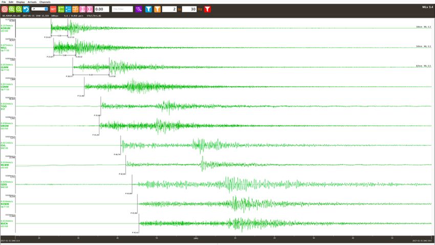
Exporting Data .................................................................................................... 22
“Save As” file and name formatting ................................................................................. 22
CSV file format ............................................................................................................. 23
Raw Text format ........................................................................................................... 24
Save Screenshot .................................................................................................. 25
Save Fourier ....................................................................................................... 25
Print................................................................................................................... 25
Close and Quit ..................................................................................................... 25
Generate Report .................................................................................................. 26
Get Waveforms .................................................................................................... 27
Edit Menu ................................................................................................. 28
Settings .............................................................................................................. 28
Display ........................................................................................................................ 28
Controls ....................................................................................................................... 29
Filter & Convert............................................................................................................. 29
Magnitude .................................................................................................................... 30
Destinations (formerly “Folders”) ..................................................................................... 30
STA/LTA....................................................................................................................... 31
Arrivals ........................................................................................................................ 32
Remove Startup Image… ...................................................................................... 32
Clip Visible to New File .......................................................................................... 32
Stack to New File ................................................................................................. 33
Set Arrival Error................................................................................................... 33
Remove Spikes .................................................................................................... 33
Display Menu ............................................................................................ 34
Zero Correction & Amplitude Grouping ............................................................................. 34
Channel Sorting ............................................................................................................ 34
Horizontal and Triaxial Peak Particle Motion Plots ............................................................... 34
Hide and Show Spectrograms and FFT/PSD....................................................................... 34
Arrivals Menu ........................................................................................... 35
Channels Menu ......................................................................................... 36
Gecko Histogram Display.......................................................................... 36
Basic Data Analysis .................................................................................. 37
The P wave ......................................................................................................... 37
The S wave ......................................................................................................... 37
Rough Magnitude Estimation ........................................................................................... 38
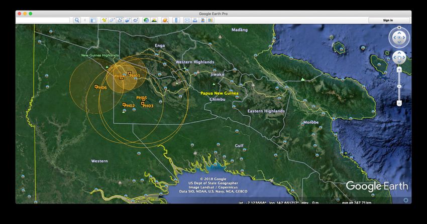
Exporting to Google Earth .............................................................................................. 39
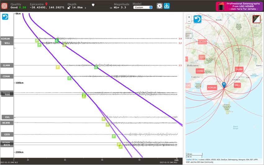
Accurate Earthquake Location & Magnitude ............................................................. 40
Location Screen ............................................................................................................ 41
Zooming and Scaling ..................................................................................................... 41
Editing Phase Arrivals .................................................................................................... 42
Earthquake Depth ......................................................................................................... 42
Location Quality ............................................................................................................ 42
Location Settings .......................................................................................................... 43
Saving the Event Location .............................................................................................. 44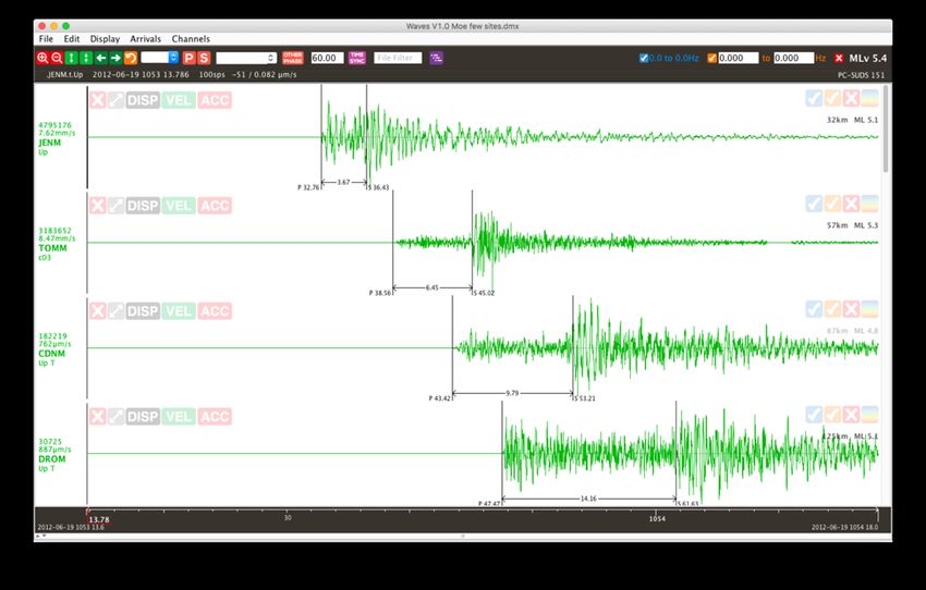
History

The Seismology Research Centre
The Seismology Research Centre (SRC) was established in 1976. In 1977 the SRC began
developing “Kelunji” digital seismic recorders, starting with the Alpha and Beta tape-based
recorders (later renamed Yerilla). The first Kelunji-branded recorder was later referred to as
the Classic, which was followed by the D-series, Echo, EchoPro, and the current Kelunji Gecko.

  Above: the original 2015 Gecko Compact seismic recorder, next to an iPhone 6 for scale

Data Formats
The Kelunji Gecko was our first recorder to natively store data in MiniSEED format. MiniSEED
data files do not include information about the recorder or sensor gains and sensitivity factors,
but the Gecko stores this information in a simple text file in each data folder. Waves will
automatically read the file if it is present, displaying your data in real ground motion units.
You can then save this extra data into the file by saving it in PC-SUDS format.

When the Kelunji D-series was introduced in the mid 1990s the SRC decided to adopt a global
standard data format for our seismic recorders. The SUDS (Seismic Unified Data System)
was originally created at the U.S. Geological Survey and adopted for use in the IASPEI
Seismological Software Library, where it became known as PC-SUDS. It is a very flexible
format which contains many fields for information relating to the raw data, which has enabled
our Waves software to provide very useful information to Kelunji users.

For more information on SUDS, visit http://banfill.net/?page_id=16

Waves can also read other data formats including: KA1, KA2, Yerilla, SEG-Y, SEG2, GSE 2.0
(AutoDRM), CSS waveform binary (.w), CSS arrival text (.wfdisc) and CSV text. Waves will
automatically decompress any files that use .zip, .gz or .xz compression.

                                               5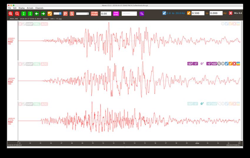
Installing Waves

Java Not Required
Waves 4.0 includes everything it needs to run as a stand-alone Windows, macOS or Ubuntu
application, so unlike previous versions of Waves you no longer need to have Oracle’s Java
Runtime Environment (JRE) installed.

Waves Workspace
When Waves starts up, you will be presented with the window below, with a toolbar containing
buttons for some commonly used function. The main workspace is where the waveforms will
appear, and below this is a pull-up window that reveals the frequency spectrum display.

Drop a MiniSEED, SUDS or other compatible file from your computer’s file browser onto the
workspace to view the waveform, then start analysing your seismograms.

                        WAVES MAIN WORKSPACE

      DRAWER SLIDER
      Drag up for frequency spectrum display

                                             6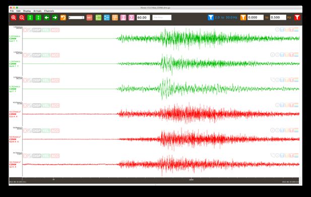
Toolbar & Channel Buttons
    Shortcut Key      Description

                      If you have 3 or more arrival picks, enter Location feature

      Page Up         Zoom in to the timeline (or zoom to selection)

     Page Down        Zoom out of the timeline (centred on click or selection)

        Home          Display full timeline and amplitude

         p, s         Select the arrival types to mark on the time line

          w           Set the arrival marker selected in the drop down list

                      Switch between Individual and Fixed Amplitude Scaling

                      Switch between Displayed and no Zero Offset correction

                      Trim the working file to only the displayed data

         ⌘-g          Display the 3D vector sum (peak particle motion)

                      Display the 2D vector sum (peak horizontal motion)

                      Enter a time correction for the selected station (seconds)
        b or n        Open next file if name includes this text, use (B)ack or (N)ext

         Sort         Re-apply the station order sorting

          g           Filter all channels using the Preset frequency band

                      Filter all channels to the Custom frequency band specified in
          h
                      fields to the right of the button

           j          Clear frequency filter from all channels

                      Per-channel filters – functions as above
         ⌘-i          Channel Information
                      Flip channel polarity (black arrow up=normal, down=reverse)
                      Show/hide channel rotation controls (coloured if changed)
                      Show/hide channel elevation controls (coloured if changed)
                      Show/hide channel spectrogram plot. Shortcut keys affect all
    k (on), l (off)
                      channels – turning all spectrograms on will take some time

                                        7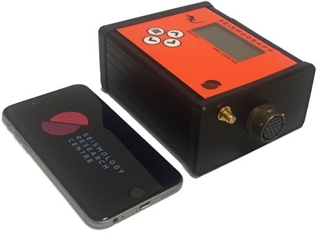
Controls
 Note:    where you see the ⌘ symbol in this manual, it represents the Control key on Windows and
          Linux, or the Command key on macOS, unless otherwise specified.

Zooming & Scrolling
All zoom commands are applied to all channels at the same time.

Scroll-zoom
While holding down the right mouse button or the CONTROL key, roll your scroll wheel to
zoom in and out to your cursor’s location on the time line. The zoom speed can be adjusted
in the “Controls” setting. Note that some touch-based pointing devices (e.g. macOS
trackpads) may not behave as expected when scroll-zooming. Double right-clicking your
mouse will reset the zoom level to the full timeline, as will clicking the   button.

Click-zoom
Clicking and dragging your cursor over the waveform will show a red vertical marker bar.
Move to the area you want to zoom into and release the cursor-click to leave a light grey
marker line. Click the      button or PAGE-UP shortcut key to zoom in to the marker or use the
   button or PAGE-DOWN shortcut key to zoom out, centred on the marker.

This zoom speed is also adjusted by the zoom “Controls” setting.

Swipe-zoom
Instead of left-clicking and dragging a marker line, you can right-click and drag to highlight
an area of interest. After releasing the click, place your cursor over the highlighted section
and you will notice that your cursor changes into a magnifying glass. Click to zoom the
highlighted area to full window width.

Timeline scrolling
Use the left and right arrows on your keyboard to scroll the time line, or holding down the
ALT key and using the scroll wheel.

Amplitude scaling
Use the up and down arrows on your keyboard to double or halve the signal amplitude of all
channels. Use the        button or HOME keyboard shortcut to revert the amplitude.

                                                8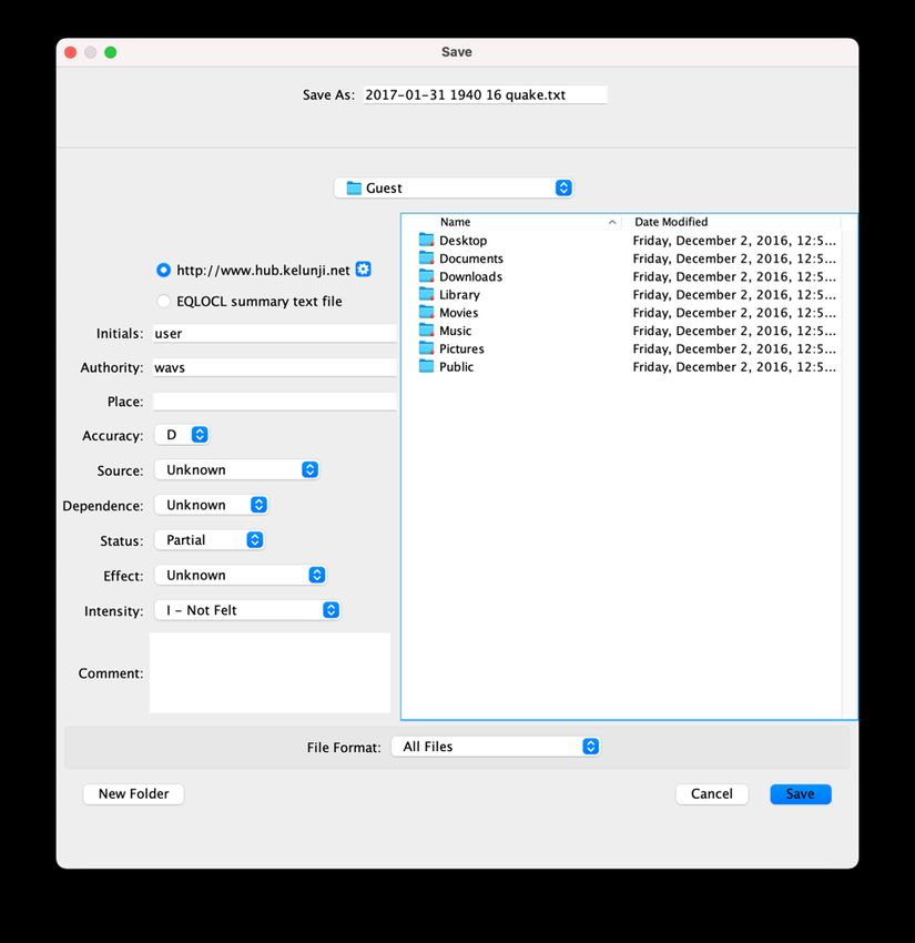
Picking Arrivals
The main function of Waves is to pick earthquake wave arrival times on the recordings to
allow the determination of the location and magnitude of the earthquake. We will cover the
basics of picking P and S wave arrivals and calculating earthquake location and magnitude
later in this user manual.

To mark a phase arrival time, click and drag the cursor to the point of interest on a channel
and release to leave a grey marker line. Select a type of arrival from the drop-down list. This
list of arrivals is based on a customisable text list in a (new to Waves 4.0) settings tab.

                                           Once the marker line is in place, click the     toolbar
                                           button (or use the W shortcut key) to mark the
                                           selected phase time on the station (or channel, in
                                           the case of X markers).

                                           You can use keyboard shortcuts to set P, S and MAX
                                           arrivals, as well as X to mark a channel stacking
                                           marker. The most commonly used seismology
                                           arrival phase codes are listed in the Arrival Settings
                                           list, but you add any text you like into the list to use
                                           as a time mark identifier.

Amplitude Grouping
To maximise the detail of the displayed data, Waves will scale the amplitude of each channel
to fill the vertical space allowed for each channel, which means each channel will have an
Individual peak amplitude scale on the Y-axis. You can choose to group the amplitudes by
Location, which will scale all channels with the same station and location code to the largest
channel’s amplitude. You can group All channels to the single largest amplitude in the file,
regardless of station code. Finally, you can scale Acceleration, Velocity, or Displacement
waveforms to a Fixed peak value as defined in the “Display” Settings.

Clicking the    button will toggle between Fixed and Individual modes, but other modes are
available in the Display menu. Channels that have been converted from their natural units
(usually velocity or acceleration) to other units will always scale individually.

                                                9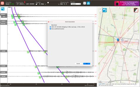
Zero Correction
When a sensor is plugged into a recorder it will almost always have some level of signal offset,
which can be due to the sensor not being perfectly level or the sensor components requiring
some sort of electronic adjustment. The raw data is never modified by Waves, only the way
it is displayed. Each channel is corrected individually. The offset correction can be based on
the zero-offset of the visible data (Displayed) or based on the average zero level of the
entire record (All), or zero-offset connection can be turned off (None), or the zero level can
be displayed as the mid-way point between the positive and negative displayed peak signal
level (Peak to Peak) by selecting the mode in the Display menu. The              toolbar button
toggles between Displayed and None.

                NONE                                       DISPLAYED

                 ALL                                      PEAK to PEAK

Trim
The     tool will delete all hidden channels and data outside the currently visible time line,
leaving you with a new file that needs to be saved separately. When using the Trim tool, the
original data file is closed, whereas when using the “Copy Visible to New File” in the Edit menu,
the original data file remains open in a window behind the new trimmed data file.

                                               10
Vector Sum
We are often using sensors that record in three dimensions, usually set up in the east-west,
north-south, and up-down axes, but sometimes they are aligned relative to a structure or
event, such as along a dam or pointing towards a blast. The peak motion from the event will
not necessarily be in one of these axes, so to calculate the peak value we can apply a 3D
vector sum formula to the data. Kelunji data is recorded in triaxial groups, or you can
manually group channels using the channel location code.
By using the button while channel is selected (or choosing “3D Peak Motion Plot” from the
Display menu, or using the ⌘-G shortcut) a new Waves window is displayed showing the peak
particle motion plots.
If the original ground motion units are known, the new window will show the vector sum in
the original units as well as the other two related units. In the example above, the original
green velocity traces have been summed, and the vector sums of the calculated displacement
and acceleration traces are also shown. Without some filtering, integrated ground motion
units (going from acceleration to velocity, or velocity to displacement) can contain low
frequency artefacts, so Waves automatically applies a 0.1Hz high pass filter to 3D plots, but
in “Filter & Convert” Settings you can set the filter band manually (leave blank for no filter).
If you only wish to see the peak motion of the two horizontal channels in the triaxial group,
use the button to display a 2D vector sum peak motion plot in the available units.
Using the “Sync” feature
Older instruments did not use GPS and relied on internal clocks for timing. Clock errors can
be corrected by time-shifting data using the “sync” feature. A Sync value from 0 to 30 seconds
shifts the data back in time, and a sync of 30 to 60 seconds will shift data forward. Enter a
value into this field and hit Enter to adjust the time line for the selected station code.
11File Filter
The File Filter field in the toolbar is linked to the file browsing tool in the File menu. If any
characters have been typed into this field, when you use the Next File (n) or Previous File
(b) commands, only valid files that contain those characters in the filename will be opened.
Leave the field blank to remove the file filter and open the next valid file in the folder.
Frequency Filters
A user will typically be interested in a
particular frequency band, so Waves allows
the definition of a blue “favourite” Preset band
pass filter. Waves also allows the user to set a
variable frequency band pass filter by typing
values into the fields to the right of the orange
button in the toolbar. The red filter button
clears the filters. The Toolbar filter buttons will
apply to all channels (or all visible channels,
according to your “Filter & Convert” Settings
which is discussed later in this user manual).
Once a filter has been applied to a channel,
the pass band is written in text to below the
channel filter buttons so that you are aware
that the data displayed has been filtered.
Viewing spectrograms is covered in more
detail later in this user manual, but note that
the frequency range of the spectrogram will
also change according to the channel filter
settings to maximise the resolution of the
visible frequencies in the spectrogram.
You can enable and disable filters on individual
channels by clicking on the small filter buttons
in the top right corner of each channel.
12To illustrate the effect of the filter when converting data between ground motion units, in the
example below the upper trace is a high gain accelerometer and the lower trace is a 1Hz
velocity sensor. Converting the acceleration trace to velocity and filtering it from 1Hz to 50Hz
yields a similar trace to the seismometer.
Removing the filter altogether shows the artefacts of integration (below, left), but setting the
low end frequency to 0.05Hz (20 seconds, below right) reveals the long period signal. Unit
conversion and frequency filtering
are very important tools in
revealing phase information.
Sometimes arrivals are clearer in
Displacement. Play with your data
and see what you can find!
Waveform Display Elements
Once you have opened a waveform file, the data will be plotted in the main Waves window
showing the full time line of available data. The basic elements of the display will be
described briefly below and expanded upon in later sections of the manual. Channel-specific
controls only appear when your cursor is hovering over the channel data. This helps to
unclutter the display when many channels are displayed.
13Decoding the Y-axis Labels
The station code is displayed
to the left of the Y-axis, with
the channel name and
location ID below it.
The colour of the text
indicates the units of the
original data (green is
velocity, red is acceleration).
The value above the station
code is the peak ground
motion amplitude of that
channel for the displayed time span of data. At the top of the Y-axis you will see a label in
black text indicating the maximum displayed units and recorder counts. In the example
above, the peak amplitude of the displayed data is 1.031mm/s but the amplitude scale clips
because the user has enabled Fixed Amplitude display mode, set to 0.5mm/s.
Display of Ground Motion Units
If a channel is recognised as having units in velocity, the trace and station code will be drawn
in green. If a channel is defined as acceleration, the trace and station code will be drawn in
red, and displacement in black.
You can convert between these units by clicking on the buttons in the top left corner of each
waveform trace. The waveform colour will change, but the station code will remain in the
original recorded unit colour. Other recognised units are pressure, rotation, and voltage.
Any unrecognised units are displayed in dark grey. The buttons will disappear
for pressure, rotation and other units as they cannot be transformed.
Minimise and Maximise Channels
To the immediate left of these ground motion conversion buttons are the minimise and
maximise buttons. Use the button to maximise the view of a channel to full screen and the
button to go back. When all channels are shown, use the button to hide that channel
from view. To restore all hidden channels, go to the Channels menu and select to show All
or show Vertical channels, or the channels of a specific site.
14Channel Rotation
If you have opened a triaxial seismogram, the North channel should show a compass
symbol, and the vertical channel should show an angle symbol. Click on the symbol to
open up the rotation and elevation adjustment controls.
The assumption is that your sensor was oriented aligned to North (0°). By clicking on the
purple degree adjustment buttons on the North channel, the seismogram will be rotated
around the vertical axis and the North and East channels will change. The rotation icon will
change from light to dark to show an adjustment has been made, even after the tool is closed.
sensor at 0° rotation sensor rotated to +45°
Similarly, by clicking on the teal elevation adjustment buttons on the Vertical channel, the
seismogram will be rotated around the North-South axis, so the Up and East channels will
change. The elevation icon will change from light to dark to show it has been modified.
N N
sensor at 0° elevation sensor elevated to +6°
15Channel Polarity
A sensor is normally set so that a positive signal equates to positive motion in the East, North
or Up direction, but this can vary due to sensor orientation or sensor wiring. If you find that
a channel has the opposite polarity, you can flip it by clicking on the button. If the black
arrow is facing up, the original data is being displayed; if the black arrow is facing down it
indicates that the reverse polarity data is being displayed.
Channel Information
Once you click on a channel its Y-axis bar will be slightly thicker than other channels to show
that information relates to this channel (e.g. the frequency spectrum display or channel
information display). When you click on the button, type ⌘-I, or select Channels ▶ Info
a window will pop up displaying extra information about this channel and its station.
The left side of the General tab has editable
elements related to the Station and Channel
codes, as well as scaling factors to allow the
raw data counts to be scaled to real-world
units. If the GPS position of the station is
available, a small marker will appear next to
the station name which when clicked will
show the station location in your web
browser using Google Maps.
You can switch to a different channel that
shares the station code and network ID using
the drop-down Channel field menu, or click
into the field to edit the channel name.
On the right side of the window an Instrument Information pane shows some recorder and
sensor parameters, such as battery voltage and temperature, serial numbers, and any other
fields that can be decoded from the data file.
If you need to modify the system response (e.g. if you have opened a data-only MiniSeed file
without an accompanying station.xml file) you can modify the displayed fields and click OK to
apply these channel settings. If you have a single “Sensitivity” value for your channel, enter
it into the “Counts Per Volt” field and put a value of 1 for “Volts Per Unit” and “Flat Gain”.
Note that Acceleration units are specified in V/m/s2, but accelerometers are usually specified
in Volts-per-g, so adjust the value accordingly. For example 10V/g = 1.0197162 V/m/s
16Poles & Zeroes
The second tab on the Info window is
labelled Poles and Zeroes and allows you
to enter the Poles and Zeroes for the sensor
channel group.
Adding this information changes the Power
Spectral Density (PSD) plot, as shown in
the images below. The left image is the raw
data with ground motion scaling only, and
the right image has the poles and zeroes
corrections applied. The raw time series
waveform data is unchanged.
Meta Data and Station.xml
The third tab will have different labels depending on the format of the data file and whether
or not it contains meta data. Kelunji D-series, Echo and EchoPro SUDS files Comments field
will be displayed in the tab, as will Kelunji Gecko settings.ss file contents.
If you have opened a MiniSEED file from a folder that also contains a related station.xml
file, the .xml file contents will be displayed in the tab. If there is no .xml file, Waves will
look up the IRIS DMC for a channel that matches the station/network/location ID and
automatically populate the meta data fields. Waves will also store the station.xml file in
your user/eqsuitefiles/response folder for future use.
Channel Filters
The next three buttons are the individual channel filter control buttons. Please see the earlier
section on Filtering to learn about the function of the blue, orange and red filter buttons.
17Spectrogram
The button will show and hide the spectrogram for a channel. This will split the waveform
area into two rows, squeezing the time series ground motion trace into the top half and the
time series frequency spectrum into the bottom half. This display mode works best when a
channel is maximised. Using shortcut key K will open the spectrogram window for all channels
(many channels can take some time), and L will close all of the spectrogram windows.
By default the scaling of the spectrogram is a log-log plot, best for looking at low frequency
signals. You can switch the spectrogram scaling to linear plots by clicking on the button
in the top right of the spectrogram, or revert to log plot by clicking the button. The
frequency or period of the data under your cursor is displayed to the left of the Y-axis of the
spectrogram: shown in Hertz when the value is above 1Hz; and shown in Period (seconds)
for values below 1Hz.
The spectrogram shows the intensity of frequency over a sampling period. If the sampling
window is too narrow you will see a vertically streaky spectrogram (below, left) and if the
sampling window is too wide the spectrogram will appear smeared over time (below, right).
You can widen or shorten the sampling window by using the and buttons until you can
see the frequency content at a usable resolution.
The spectrogram colours scale to the highest intensity of the displayed data, which can
dominate the plot during an earthquake, which can obscure the pre-event and post-event
frequencies. You may
want to see if there is a
change in the natural
frequency of your
building, which means
looking for a shift in this
resonance before and
after an earthquake.
Use the and
buttons to increase or
decrease the frequency
intensity level.
18Frequency and Power Spectrum Display
Press the F shortcut key to toggle the frequency display window open or closed, or drag up
the horizontal divider bar at the bottom of the Waves window. You can adjust the size of this
window by dragging the divider bar up or down. Initially it will display a linear-scaled Fast
Fourier Transform (FFT) frequency spectrum of the currently selected data.
Right-click any channel to display the frequency spectrum for the full time series, or right-
click-and-drag to see the frequency spectrum of a selected time period. Note that the selected
channel has a thicker Y-axis bar and is named in the top left corner of the FFT window. You
can click and drag over a section of the frequency plot, then place your pointer over the
highlighted section and click to zoom in for a more detailed view.
In the top right corner of the FFT window you’ll
see a toolbar that allows you to edit the view and filter the data. The magnifying glass icon
will reset the zoom to the full frequency range.
Filtering in the Frequency Domain
The button in the frequency window tool bar displays the FFT on a linear frequency scale.
Clicking on the button when displaying linear FFT will change the graph to a log-log plot.
You can use this FFT window to filter your data. Right-click and drag to select a frequency
range, then click the to keep only that frequency range. The time series data will then be
redrawn based on the filtered frequency data.
Conversely, click the after
highlighting a frequency range to
reject the selected range.
In the example shown, inadequate
shielding from AC power results in
50Hz noise dominating the signal.
By click-and-dragging over the
anomalous frequency band and
clicking the button in the top
right of the FFT window, the
highlighted region is dropped out
and the time series waveform is
then redrawn.
19The notch filter can be applied repeatedly over the frequency spectrum, as shown below.
To clear all filters from the channel, click the button in the FFT window or on the channel.
Power Spectral Density Plot
While you are viewing the FFT log
plot, click the button again and
the graph will toggle to a Power
Spectral Density (PSD) plot. The
horizontal range of this log-scale
plot shows data from a long
period to the decade above the
Nyqvist frequency. If a band pass
filter has been applied, the
horizontal scale will span the
decades either side of the pass
band.
The button shows the PSD
relative to the Peterson New Low
Noise Model (NLNM) and New
High Noise Model (NHNM) curves,
from 1000 seconds to 10Hz. You
can still zoom and filter the
frequency range in the PSD and
Peterson Model plot views.
This gives you an idea of the
noise level of your station.
20File Menu
Opening and Closing Files
You can drag a file from your computer’s file browser onto the Waves window to view it.
You can also use the File ▶ Open menu item (⌘-O) to browse your computer for your file.
To close the file and go back to an empty Waves window use the operating system’s window
close button, File ▶ Close menu item, or ⌘-W.
When you have a file open, you can open another file by dragging it onto the Waves window
or using the Open command again, but this will open the file in a new Waves window. If you
would like to merge the additional files into the same Waves window, read on.
Merging Files
Waves can merge up to 24 hours of data from many stations into a single file. Kelunji seismic
recorders store continuous data in one-minute-long data files, so it is possible that an
earthquake recording will straddle two or more files. To make analysis easier you can merge
these files together on screen and then save the merged file to your computer.
The quickest way to merge several files into a single viewer window is to multi-select files in
your operating system and drag them into the Waves window while holding down the Control
key on Windows or macOS, or the Shift key on Linux.
Alternatively, use the File ▶ Open command, select the files you wish to merge using your
multi-select file system shortcuts (usually Shift, ⌘ Command or Option-clicking) and tick the
“Merge into current file” checkbox before clicking the button to proceed.
21Merging Folders
If you File ▶ Open on a folder or drag a folder containing files onto Waves, all of the contents
of the folder (and sub-folders) will be merged into a single (24-hour maximum) timeline. This
is a quick way to view an entire hour or day folder from a Gecko’s SD card.
When merging, as long as all of the files are within a 24-hour time period, they will be merged
onto a common time line, grouped by site code in alphabetical order. Your computer’s memory
will limit to how much data is practical to open in a single window, which will depend on
sample rate, number of stations, and number of channels.
Exporting Data
To quickly save a file to your last “Save As…” folder for later review, use the File ▶ Auto Save
(Y) command. This is useful when you are reviewing a folder full of seismograms using the N
and B shortcuts and you come across a file that you would like to review in detail a bit later.
After quick-saving, Waves will automatically open the next file in the folder.
Once you have merged, clipped, or modified your seismogram file you can save it using the
File ▶ Save command or ⌘-S. This will overwrite the file whose name is displayed in the title
bar or the Waves window.
“Save As” file and name formatting
If you do not wish to overwrite the file, you can use File ▶ Save As or ⌘-T to save your data
to a new file. In the Save dialog box that pops up there are control options for naming the
file. The “SRC” filename format follows the form: YYYY-MM-DD hhmm ss STATION
If you are saving a merged file the STATION code in the file name will be one of the channels
from the recording, depending on the order in which they were merged by the system.
If you decide to use the “GA” filename format, the file will be named in the form
SITEYYDDD_hhmmss where YY is the last two digits of the year (e.g. 13 for 2013) and DDD
is the day number of the year (i.e. 001 to 366).
By default Waves will save files in gzip compressed PC-SUDS format (file extension: .dmx.gz)
which embeds station data in the file format. You can also save as a MiniSEED zip file, which
creates a zip compressed folder containing the MiniSEED waveform and a companion text file
with the station response. Waves can them open compressed files and automatically apply
the station corrections. Other text based formats are available, which can be imported into
spreadsheets, text processors, or mathematical processing and plotting applications.
See “Basic Analysis” later in this manual to understand how saving a .kml format file from a
multi-station waveform with P & S picks can be used to estimate the earthquake epicentre.
22CSV file format
When you save your seismogram as a CSV file, it is in ASCII format using commas for
separating the values in the file. CSV files are easily read using Excel.
It contains a header that describes the Arrivals contained in the file, a section that describes
the time series data in the file, followed by the data points.
Any arrival information contained in the seismogram will be listed in the first section. Each
arrival will have its own column detailing the site name, arrival type and time.
The next section describes the time series data, one channel per column. This includes the
site name, channel name, the date and time of the first data point (or “sample”), and how
many samples there are per second. As you may have merged data of differing sample rates,
there may be a variable number of rows per column for a given time period.
The final row before the data points indicates the units of the data, which could be metres
(m), metres per second (m/s), metres per second squared (m/s/s), etc. The data is then
displayed in these units, one sample per row. All data is saved with zero-offset correction.
#csv file
ARRIVALS
PH01,PH01,PH01,#sitename
, , ,#onset
, , ,#first motion
P,S,AML,#phase
20180407,20180407,20180407,#year month day
0548,0548,0548,#hour minute
46.469,51.102,46.469,#second
0.005,0.005,0.100,#uncertainty in seconds
, , ,#peak amplitude
, , ,#frequency at P phase
TIME SERIES
PH01,PH01,PH01,#sitename
HNE _,HNN _,HNZ _,#component
_,_,_,#authority
20180407,20180407,20180407,#year month day
0548,0548,0548,#hour minute
42.839,42.839,42.839,#second
200.00,200.00,200.00,#samples per second
4258,4258,4258,#number of samples
0.000,0.000,0.000,#sync
m/s/s,m/s/s,m/s/s,
--------,--------,--------,
-0.0006709909,0.0018134047,-0.0010640614,
-0.0006945866,0.0019957353,-0.0011305584,
-0.0007632287,0.0021609052,-0.0012978734,
… more data
0.2632255554,0.4593577981,0.0390293375,
0.2496086955,0.4775865674,0.0227354281,
0.2339282781,0.4935994744,0.0048155603,
, , ,
END,END,END,
23Raw Text format
When you save your seismogram as a text file, the fields are tab separated and the data is in
raw integer counts as stored by the recorder (not zero-offset corrected by Waves). The
conversion factors are listed in the TIME SERIES header section to allow you to turn raw
counts into ground motion values. Convert using the operation:
counts ÷ Counts/Volt ÷ Volts/Unit ÷ Flat Gain = units
e.g. 2835 ÷ 419430.4 ÷ 1.02 ÷ 1.09 = 0.0060794807 m/s2 (620µg)
ARRIVALS
PH01 PH01 PH01 #sitename
#onset
#first motion
P S AML #phase
20180407 20180407 20180407 #year month day
0548 0548 0548 #hour minute
46.469 51.102 46.469 #second
0.005 0.005 0.100 #uncertainty in seconds
----- ----- ----- #peak amplitude
----- ----- ----- #frequency at P phase
TIME SERIES
PH01 PH01 PH01 #sitename
HNE _ HNN _ HNZ _ #component
_ _ _ #authority
20180407 20180407 20180407 #year month day
0548 0548 0548 #hour minute
42.839 42.839 42.839 #second
200.00 200.00 200.00 #samples per second
4258 4258 4258 #number of samples
0.000 0.000 0.000 #sync
m/s/s m/s/s m/s/s #units
419430.4 419430.4 419430.4 #Counts/Volt
1.020 1.020 1.020 #Volts/Unit
1.090 1.090 1.090 #Flat Gain
-22.2222 -22.2222 -22.2222 #latitude
147.4747 147.4747 147.4747 #longitude
counts counts counts
-------- -------- --------
2835 -4858 942
2824 -4773 911
2792 -4696 833
2742 -4568 764
… more data
134228 193893 33672
130927 200633 27422
125860 208443 19633
119512 216941 12037
112202 224406 3683
END END END
24Save Screenshot
Although most computers have a screenshot feature, Waves allows you to save
a PNG format image of just the data window, excluding the control panel and
window frame. If you have many channels in the scrolling window, the screenshot
will be very tall.
Computer window screenshot (above) vs. a Waves window screenshot (right)
Save Fourier
You can also save the data that is displayed in the Fourier transform window to
a text file. Right-click on a channel to display the frequency spectrum for the
entire channel recording, or right-click and drag a portion of the data you wish
to analyse and its frequency spectrum will appear in the Fourier window.
By selecting File ▶ Save Fourier the data that is being displayed in the Fourier
transform window will be output in three columns, the first showing the frequency
point (in Hz) followed by the real and imaginary values of the spectrum.
Print
If you would like to print your waveform you can use the File ▶ Print or ⌘-P
command. It will print effectively the same information as the Waves screenshot,
except that it will print up to 9 channels per page to the maximum scale to fill
the page.
Close and Quit
Close the Waves window using File ▶ Close or ⌘-W to return to an empty Waves
window. Use this command again or File ▶ Quit or ⌘-Q at any time to quit
Waves.
25Generate Report
More and more, Gecko recorders are being used for
monitoring blasts and vibrations in mines, quarries, and
from civil construction and demolition works.
Extraordinary events often require a summary report of
the data recorded to show whether the ground motion
and air pressure vibrations were within permitted levels.
While viewing an event recording in Waves, use
the File ▶ Generate Report option to open a
dialogue box that allows you to customise the
content of the report.
You can set a logo to appear on the report, and
it will be saved for future reports. Use a JPG or
PNG file. It will be rescaled to fit a 120x90 pixel
area. The title of the report can also be modified
and will also be retained for future reports.
Waves Blast Report
Three free text fields are available per
report. Site and Location are 20-
Time: 2021-05-21 09:48 AM AEST
2021-05-20 2348 05 (UTC+10) Site Name: Hunter Region
Recorder: GECKO Location Name: 1km NW of main pit
character fields, and you can enter
3D Sensor: Miniseis Geophone #0 Latitude: -32.82146
1D Sensor: Miniseis Microphone #0 Longitude: 151.57190
Notes: No reports from local residents
about 300 characters in total that will
3 appear over three lines in the Notes
3D sensor X
2.028 mm/s
mm/s
field. All of these text fields appear in
0
01:54PM 33.189
0.0Hz to 250.0Hz
-3
3
3D sensor Y
1.445 mm/s the header of the report.
mm/s
0
01:54PM 32.787
0.0Hz to 250.0Hz
-3
3
3D sensor Z The check-boxes allow you to select
1.290 mm/s
mm/s
0
01:54PM 31.669
-3
0.0Hz to 250.0Hz
which sections to include in the
3
3D sensor vector
2.323 mm/s
report, and the Fourier Spectrum
mm/s
01:54PM 33.361
0.1Hz to 250.0Hz
115
1D sensor
section allows you to select an upper
114.988 dB
dB
0
limit to the frequency plot (X) axis to
01:54PM 37.727
0.0Hz to 250.0Hz
-115
show more detail in the lower
26 27 28 29 30 31 32 33 34 35 36 37 38 39 40 41 42 43 44 45 46 47 48 49 50 51 52
2021-05-13 13:54:25 AEST (UTC+10)
3D sensor X
2.028 mm/s
11.22 Hz frequency range. Depending on your
sample rate, the plot limit options will
3D sensor Y
1.445 mm/s
10.12 Hz
be to 25Hz, 50Hz, 100Hz, 250Hz and
3D sensor Z MAX (half the sample rate).
1.290 mm/s
10.97 Hz
A sample of the waveform and
1D sensor
114.988 dB
10.21 Hz Fourier Spectra plots from the report
is shown at left.
26The second page of the report, if enabled,
will show a “Zero-Crossing” plot in the Waves Blast Report
Time: 2021-05-21 09:48 AM AEST
2021-05-20 2348 06 (UTC+10) Site Name: Hunter Region
style of the USBM RI8507 chart. This is a Recorder: GECKO
3D Sensor: Miniseis Geophone #0
Location Name:
Latitude:
1km NW of main pit
-32.82146
1D Sensor: Miniseis Microphone #0 Longitude: 151.57190
simplified method of plotting velocity Notes: No reports from local residents
amplitudes by calculating the peak’s
frequency based on the time between the
waveform crossing the zero-line. The plot
frequency range is fixed from 1-100Hz
and the particle velocity range is from 1-
110mm/s. The standard threshold levels
for residential structure damage potential
is overlaid as a guide to the safe blasting
and vibration levels.
If the 3D and 1D sensor name and serial
numbers are available, these will be
added to the header, along with the
geographic location of the station – click
the pin icon to open in Google Maps.
Get Waveforms
If data from your seismic monitoring network is being received by the SRC eqServer
earthquake observatory data management system, you can extract waveform data from that
archive directly from Waves without having to log in to eqServer using a web browser.
Click on the cog symbol to view the eqServer settings to enter the web address and login
credentials of your eqServer. Once connected, set the date, time, and length of the data
extraction request. If you leave the station and radius fields empty, all data on the server for
that time will be returned, or enter a station code to only return data from stations within the
nominated radius of that station. Once extracted, the seismograms will appear in your Waves
window, ready for analysis.
27Edit Menu
Settings
Display
The first setting in this tab
relates to the way the time is
displayed. By default Waves
displays data in UTC time,
but if your recorder uses a
UTC offset to define local
time for file names, you can
choose to display data using
the stored UTC offset
(Recorder Setting) or you
can get Waves to always
display data with a Custom
UTC Offset (e.g. +10.0
hours for Australian Eastern
Standard Time).
There is a minimum vertical space required by Waves to draw a channel, but you can also set
it to display a maximum number of channels, for example if you wish to display only 3 or 6
channels on screen at a time. Enter the maximum number of channels you wish to display in
the field shown. The remainder of the channels are accessible by scrolling.
When displaying pressure (usually a recording from a microphone), Waves can display
amplitude in Pa (pascal) or as SPL (sound pressure level, measured in dB). When plotting
acceleration, Waves can display amplitude in g (gravity), in m/s2 (metres per second squared,
shown as mm/s2 or nm/s2 as required) or in gal (cm/s2).
As discussed in the Toolbar section on Amplitude Grouping, you can fix the amplitude scale
for native acceleration, velocity and displacement data. These fixed values are defined for
acceleration, velocity and displacement using the values you enter in the boxes.
When your final waveform is closed, an empty Waves window remains. This empty workspace
can be hidden so that only the toolbar remains.
When you mark a P-wave arrival time and an S-wave arrival time, Waves can display the
time difference. You can turn the “Show S minus P” feature on and off with the checkbox.
28Controls
As discussed in the section on Zooming,
the speed of zooming can be
customised. This affects the step size of
the incremental zoom when using the
toolbar buttons or keyboard shortcuts,
and also the speed of zooming when
using the scroll wheel while holding
down the right-mouse-button or
CONTROL key.
The size of the steps used to horizontally
scroll the time line (by using the toolbar
buttons or keypad arrows) can also be
adjusted. This also affects the speed of timeline scrolling when using the mouse scroll wheel
while holding down the ALT key.
Some pointing devices such as multi-touch trackpads can behave erratically when zooming
or scrolling. A scroll-wheel mouse is recommended for the best user experience.
Filter & Convert
You can set the pass band of the
frequency range of your favourite Preset
filter here. Once defined, these values
are displayed in blue in the toolbar.
The Toolbar filters buttons can apply to
all channels or just those that are
currently visible.
When the 2D or 3D vector sum peak
particle plots are performed, the
integrated data (converting from
acceleration to velocity, or from velocity
to displacement) can be affected by
conversion artefacts that usually need to be filtered out.
This group of settings allows you to choose to automatically apply a preset pass band filter to
manually integrated data (when you press the channel buttons, to one all or
all grouped channels), or integrate the data based on the current frequency range, which may
or may not be filtered.
29Magnitude
The P wave and S wave velocity values are used by a simplified method to estimate an
earthquake’s distance from a station. You can set a single P and S velocity and typical
earthquake depth to suit your local region. Changing these will affect the distance and
magnitudes calculations.
The default formula for local Richter magnitude is:
log(A*2080)+log(D)+0.00301*D+0.7 where A is
amplitude of the peak displacement of the vertical
channel (in millimetres, after being filtered by the
customisable high pass filter, default is 2.0Hz+)
and where D is the estimated distance from the
station to the earthquake based on the P & S picks
and velocities. You can modify this formula using
standard mathematical operations and the A & D
variables.
These velocities and magnitude formula are not used by the Location feature introduced in
Waves 4.0. It only applies to the time series waveform view for rapid magnitude estimation.
Destinations (formerly “Folders”)
You can set Waves to always use a particular folder when opening, saving or quick-saving
files. Leaving the boxes unchecked will usually set the destination as the last folder used.
Here you can also define the login details of an eqServer from which you can extract waveform
data or to which you can save earthquake location solutions. This tab also allows you to define
which FDSN server to search for station response data (Waves was previously hardwired to
searching the IRIS server).
30STA/LTA
You can modify the STA/LTA settings to help
tune a Gecko recorder’s trigger routine. After
changing one of the settings, click the Apply
button to see the effect on the yellow
STA/LTA ratio plot on the waveforms if you
have this display enabled.
The yellow trace overlaid on your ground
motion recording is the simulated STA/LTA
ratio, which shows you how a Gecko
recorder’s STA/LTA trigger algorithm would
see this data with and without recorder’s
STA/LTA filter active. eqServer uses a
different STA/LTA algorithm to analyse
incoming streaming data, so this STA/LTA
ratio can also be simulated in Waves. The simulated STA/LTA ratio can be toggled on and off
by pressing the “A” keyboard shortcut.
STA stands for Short Term Average and LTA for Long Term Average. The STA/LTA Ratio is
the average signal level over a short time period (e.g. 2 seconds) compared to the average
signal level over a longer time period (e.g. 20 seconds). The ratio of the STA level to LTA
level is plotted in yellow on the screen. The scale of this plot is related to the STA/LTA ratio
trigger Threshold, which is a level at which you would expect the seismic recorder to declare
that an event is happening. The trigger threshold is plotted at the zero-level of the channel,
so the Y-axis range is a ratio of zero to twice the threshold level.
In the example below, the STA setting is 1 second, the LTA is 20 seconds, and the threshold
is 3.0. Before the earthquake the STA and LTA values are similar and the ratio of the short
term average signal divided by the long term average signal is around 1, but as soon as the
earthquake/blast hits, the average signal level in the STA period is many times larger than
the average signal in the LTA’s previous 20 seconds, so the ratio shoots through the threshold.
At this point the recorder would declare a “trigger” and perform any related actions.
31Arrivals
The list of arrival phases in the drop-down list in the toolbar is populated by a default list of
commonly used phases. These are simply text fields that are assigned to the Set marker.
You can add or remove phases from the toolbar’s drop-down list by editing this text field.
Remove Startup Image…
Waves is a free software application that is supported by a 10-second advertisement when
the program starts. If you have purchased a product key to remove the pop-up ad, you can
enter the code by selecting this menu item or by clicking on the advertisement. Your computer
must have Internet access to confirm the validity of your key with our register. Please note
that a key can only be used once and is locked to the computer user profile that activates it.
Note that this will not remove the small advertisement that is in the toolbar of the Location
feature that was launched in Waves 4.0.
Clip Visible to New File
You may wish to create a new seismogram file with a subset of the data in the currently-
displayed Waves data file. You can remove channels or restrict the time period so that you
are only left with data relevant to your analysis requirements. The Edit ▶ Clip Visible to
New File menu item (also accessible using the ⌘-L keyboard shortcut) will open a new
window that contains only the data visible in the vertically scrolling main window in Waves.
This means that any channels that have been hidden will not be exported to the new window,
and only the data from the current timeline zoom level will be exported to the new window.
Filter settings will be carried across to the new window, although they can be cleared so that
the original raw data can be displayed.
32Stack to New File
Seismic recording equipment can be used in exploration applications as well as earthquake
seismology. It is not uncommon to record dozens of vertical geophones over a small area to
improve the signal-to-noise ratio to better see events.
The method of “stacking” waveforms helps to reduce the random noise as it does not correlate
from sensor to sensor, whereas the event signals do correlate.
By marking a common arrival phase on each channel using the X keyboard shortcut then
initiating the “Stack” menu command, a new window will appear with the waveforms stacked
onto the earliest X marker.
Set Arrival Error
After picking P or S arrival, you can right-click and drag to highlight a time span around the
marker to indicate your range of uncertainty around your time pick.
By then using the “E” keyboard shortcut or selecting the “Set arrival error” item from the Edit
menu, the arrival will then be assigned an uncertainty of the greatest deviation from the pick
time in your highlighted section. If your earthquake location supports it, this uncertainty value
can be assigned to the phase time and weighted accordingly in the location algorithm.
If you mark a P or S arrival time, the default uncertainty will be the time equivalent of two
data samples (i.e. ±0.02 seconds for data recorded at 100 samples per second).
If you mark the arrival as an impulsive i+P, i-P or iS, the default uncertainty will be one data
sample (i.e. ±0.01 seconds for data recorded at 100 samples per second).
If you mark the arrival as an emergent eP or eS, the default uncertainty will be ten data
samples (i.e. ±0.1 seconds for data recorded at 100 samples per second).
Remove Spikes
In digital data it is possible that one or more sequential samples can become corrupted,
presenting a “spike” in the data. This feature attempts to correct the data corruption.
33You can also read