Ascertaining price formation in cryptocurrency markets with Deep Learning
←
→
Page content transcription
If your browser does not render page correctly, please read the page content below
Ascertaining price formation in cryptocurrency markets with Deep
                                           Learning

                                           Fan Fanga , Waichung Chungb , Carmine Ventrea , Michail Basiosc,d , Leslie Kanthanc,d ,
                                           Lingbo Lid , Fan Wud
arXiv:2003.00803v1 [q-fin.GN] 9 Feb 2020

                                           a
                                               King’s College London, UK; b University of Essex, UK; c University College London, UK;
                                           d
                                               Turing Intelligence Technology Limited, UK

                                                 ARTICLE HISTORY
                                                 Compiled April 6, 2020

                                                 ABSTRACT
                                                 The cryptocurrency market is amongst the fastest-growing of all the financial markets in the
                                                 world. Unlike traditional markets, such as equities, foreign exchange and commodities, cryp-
                                                 tocurrency market is considered to have larger volatility and illiquidity. This paper is inspired
                                                 by the recent success of using deep learning for stock market prediction. In this work, we an-
                                                 alyze and present the characteristics of the cryptocurrency market in a high-frequency setting.
                                                 In particular, we applied a deep learning approach to predict the direction of the mid-price
                                                 changes on the upcoming tick. We monitored live tick-level data from 8 cryptocurrency pairs
                                                 and applied both statistical and machine learning techniques to provide a live prediction. We
                                                 reveal that promising results are possible for cryptocurrencies, and in particular, we achieve a
                                                 consistent 78% accuracy on the prediction of the mid-price movement on live exchange rate
                                                 of Bitcoins vs US dollars.

                                                 KEYWORDS
                                                 Cryptocurrency; Deep learning; Prediction

                                           1.      Introduction

                                           How algorithmic traders use impartial deep learning model and get an efficient prediction of
                                           price change is an important question for algorithmic trading. This paper focuses on effec-
                                           tively applying deep neural network on cryptocurrency market trading systems. Our objective
                                           is to predict the price changes; we consider both binary (up/down) and multi-class (e.g., de-
                                           grees of increase/decrease) prediction of price changes.
                                              The cryptocurrency market is a huge emerging market (Ahamad et al. 2013). There were
                                           over 11, 641 exchanges available on the internet as of July 2018 (En.wikipedia.org 2018).
                                           Most of them are exchanges of small capitalisation with low liquidity. Exchanges with the
                                           highest 24-hour volume are FCoin, BitMEX, and Binance. Bitcoin, as the pioneer and also
                                           the market leader, has a market capitalization of over 112 billion USD, and a 24-hour volume
                                           over 3.8 billion USD in early July 2018. The cryptocurrency market is one of the most rapidly
                                           growing markets in the world, and are also considered one of the most volatile markets to trade
                                           in. For example, the price of a single Bitcoin increased significantly, from near zero in 2013
                                           to nearly 19, 000 USD in 2017. For some alt-coins, the price can increase or fall over 50%

                                                Contact Author. Email: fan.fang@kcl.ac.uk
within a day. Therefore, having a method to accurately predict these changes is a pervasive
task, but one that could achieve a long-term profit to cryptocurrency traders.
There are a number of research papers that studied the structure of the limit order book
(i.e., the bids at both sides of the market) and, more generally, the micro-structure of the
market by using different methods ranging from stochastic to statistical and machine learning
approaches (Huang et al. 2005; Altay and Satman 2005; Fletcher 2012; Biais et al. 1995).
The objective is to understand the way prices at either side of the market move; motivated by
related literature we focus on a particular measure, the mid-price, which intuitively captures
the average difference between the best ask (the lowest price sellers are willing to accept) and
best bid (the highest price buyers are willing to pay). Towards this aim we could, for example,
use Markov chains to model the limit order book (Kelly and Yudovina 2017). We could view
the limit order book as a queuing system with a random process and use birth-and-death
chains to model its behaviour. From this perspective, a very intuitive way to explain the mid-
price movement is to consider the value of the mid-price as the state of the chain. This value
is controlled by the ratio between the probability of birth transitions p and the probability of
death transitions q . A ratio p/q greater than 1 within a short interval of time indicates that
there is a higher chance for birth transitions to happen (more buyers), and the value of the
mid-price is expected to increase. Similarly, if the ratio is smaller than 1, the value of the
mid-price is expected to decrease (Sundarapandian 2009). The problem with this approach is
the way it models the order book, namely, is the limit order book a queuing system? Even if
it were, how to correctly simulate the random process and how to accurately estimate p and q
become vital questions, with unclear answers, for this approach.
In this research, we propose to adopt a deep learning approach to reveal useful patterns
from the limit order book. We give answers to a number of very specific technical questions
that have to do with this approach; our findings pave the way to the design of novel trading
strategies and market estimators. A notable finding is that we can tweak the deep learning
tools to achieve a consistent 78% accuracy on the binary prediction of the movements of the
mid-price on the live exchange of BTC-USD.
1.1. Related work
Since the birth of the market, traders have been trying to find accurate models to use to make
a profit. Many studies and experiments have been conducted based on statistical modelling of
the stock price data. Some studies attempted to model the limit order book by using statisti-
cal approaches, such as using Poisson Processes and Hawkes Processes to estimate the next
coming order and to model the state of the limit order book (Abergel and Jedidi 2015; Toke
and Pomponio 2012).
Others have used machine learning approaches to estimate the upcoming market con-
dition by applying different machine learning models, such as support vector machine
(SVM) (Kercheval and Zhang 2015), convolutional neural network (CNN) (Tsantekidis et al.
n.d.), and recurrent network such as Long-Short-Term-Memory (LSTM) (Dixon 2018). These
studies show that it is possible to use a data-driven approach to discover hidden patterns within
the market. In particular, Kercheval and Zhang (2015) modelled the high-frequency limit or-
der book dynamics by using SVM. They discovered that some of the essential features of
the order book lie on fundamental features, such as price and volume, and time-insensitive
features like mid-price and bid-ask spread. In a more recent work, Sirignano and Cont (2018)
also suggested that there might be some universal features on the stock market’s limit order
book that have a non-linear relationship to the price change. They tried to predict the mid-
price movement of the next tick by training a neural network using a significant amount of
2stock data. Their findings suggest that instead of building a stock-specific model, a universal
model for all kinds of stock could be built.
Most of the studies in the area focus on the traditional stock market like NYSE and NAS-
DAQ (Güresen et al. 2011). Many researchers have studied these exchanges for many years.
The quality of data and the market environment are more desirable than those of the cryp-
tocurrency market. Although the traditional stock market may provide a less volatile and
more regulated environment for traders, the high volatility of the cryptocurrency market may
provide a higher potential return. Our research aims to apply the same philosophy to the
cryptocurrency market and replicate the findings above. In other words, we try to model the
cryptocurrency market by using a data-driven approach. In this paper, experiments are focus-
ing on the engineering side of this approach.
Understanding price formation through mid-price for cryptocurrencies becomes even
harder due to the fact that they are distinct from traditional fiat-based currencies. The lat-
ter are usually issued by banks or governments. The only way to create Bitcoins, the currently
dominant cryptocurrency, is to run a computationally intensive algorithm to add new blocks
to the blockchain. People who participate in this processing will verify transactions on the
blockchain, and try to earn Bitcoins as the reward of adding new blocks. These people are
usually referred to as Bitcoins miners. The protocol of the Bitcoin fixed its total supply at
21 million (Nakamoto 2008). Every transaction on the blockchain is protected by a crypto-
graphic hash algorithm called SHA-256. It is a computational intensive hash algorithm that
is implemented to verify blocks on the blockchain. For instance, if a counterfeiter wants to
forge a block on the blockchain, they will also need to redo all the hashing before that block.
This property provides a trustless foundation for Bitcoin because neither an individual nor an
institution can counterfeit the currency or the transaction unless it has a computational power
in excess of the majority of the network (Nakamoto 2008).
Multi-label prediction is widely used in image processing, character recognition and fore-
casting of decisions or time series. Complex trading strategies might require more than binary
classification. One may use the status box method to measure different stock statuses such as
turning point, flat box and up-down box (Zhang et al. 2016) in order to reflect the relative
position of the stock and classify whether the state coincides with the stock price trend. In
this research, we propose to use the transaction fee as a threshold to decide whether the des-
ignated cryptocurrency market has a long or short signal. When prediction of price movement
is under transaction fee, it means in the next trading cycle the market falls in a ’Buffer area’
where the market is in a relatively stable position.
1.2. Roadmap
The paper is organized as follows. In Section 2, we provide a brief overview of the tools
adopted, including deep learning, limit order books and data sources we used. In Section
3, we design experiments to address our research questions. In Section 4, we give a brief
discussion of the validity of our findings. Section 5 gives a conclusion of this paper.
2. Our tools
In this section, we first review the background of deep learning and limit order books, before
introducing an overview of the trading system where our prediction model is trained on.
32.1. Deep Learning
Artificial neural networks are computational algorithms mimicking biological neural systems,
such as the human brain. These algorithms are designed to recognize and generalize patterns
from the input, and remember them as weights in the neural network. The basic unit of a
neural network is a neuron; a simple neural network, which is a conglomeration of neurons,
is called Perceptron.
The network used in this paper is a type of recurrent neural network called Long-Short-
Term-Memory (LSTM) (Hochreiter and Schmidhuber 1997). This is distinct from the feed-
forward neural network such as Perceptrons, since the output of the neural network sends
feedback to the input and affects the subsequent output. Therefore, LSTM is better suited for
handling sequential data where the previous data can have an impact on subsequent data; this,
in principle, works well for time series data for price prediction and forecasting.
Figure 1.: An overview of an LSTM cell
An LSTM cell contains a few gates and a cell status to help the LSTM cell decide what
information should be kept and what information should be forgotten. As a result, the LSTM
cell can recall important features from the previous prediction by having a cell state. An
LSTM cell can also be viewed as a combination of a few simple neural networks, each of
them serving a different purpose. The first one is the forget gate (Hochreiter and Schmid-
huber 1997). The previous output is concatenated with the new input and passed through a
sigmoid function. After that, the output of the forget gate, ft , will perform a Hadamard prod-
uct (element-wise product) with the previous cell’s state. Note that ft is a vector containing
elements that have a range from 0 to 1. A number closer to 0 means the LSTM should not
recall it, whilst a number closer to 1 means the LSTM should recall and carry on to the next
operation. This process helps the LSTM select which elements are to forget and remember,
respectively. The second one is the input and activation gates (Hochreiter and Schmidhuber
1997). This process concatenates the previous output with the new input, determines which
element should be ignored, and updates the internal cell state. The cell state is then updated
by a combination of the output and a transformation of the input. The third one is the output
gate (Hochreiter and Schmidhuber 1997). This process helps determine the output of the cell.
Finally, the output of the LSTM cell is the Hadamard product of the current internal cell state
and the output of the output gate (Christopher 2015; Adam 2015).
We use Root Mean Square Propagation (RMSprop) (Tieleman and Hinton 2012) – a
4stochastic gradient descent optimizer – to train the neural network, with the learning rate
divided by the exponentially weighted average. Optimizer, learning rate and loss function are
core concepts in deep learning models. Optimizer ties together the loss function and model
parameters by updating the model in response to the output of the loss function. Loss function
is a method of evaluating how well your algorithm models your dataset, which tells the opti-
mizer when it’s moving in the right or wrong direction. The learning rate is a hyperparameter
that controls how much to change the model in response to the estimated error each time the
model’s weights are updated.
In our experiments, we also tested the use of an adaptive moment estimation, Adam in
short, as the optimizer. While we observed that Adam helps the neural network to converge
faster, we noted a tendency to overfit the data; the validation set has an increasing loss while
the training set has a decreasing loss. This motivates our choice of RMSprop as optimizer.
2.2. Limit Order Books
The limit order book is technically a log file in the exchange showing the queue of the out-
standing orders based on their price and arrival time. Let pb be the highest price at the buy
side, which is called the best bid. The best bid is the highest price that a trader is willing to
pay to buy the asset. Let pa be the lowest price at the sell side, which is called the best ask.
The best ask is the lowest price a trader is willing to accept for selling the asset.
The mid-price of an asset is the average of the best bid and the best ask of the asset in the
market.
(pb + pa )
Mp = .
2
There are other metrics that are also useful for describing the state of the limit order book:
Spread, Depth and Slope.
2.3. Data source and overview of the envisioned trading system
Numerous exchanges provide Application Programming Interface (API) for systematic
traders or algorithmic traders to connect to the exchange via software. Usually, an exchange
provides two types of API, a RESTful API, and WebSocket API. Some exchanges also pro-
vide a Financial Information eXchange (FIX) protocol. In this study, a WebSocket API from
an exchange called GDAX (Global Digital Asset Exchange) is used to retrieve the level-2
limit order book live data (GDAX 2018). The level-2 data provides prices and aggregated
depths for top 50 bids and asks. GDAX is one of the largest exchanges in the world owned by
the Coinbase company.
Our focus is to design a model that can successfully predict the mid-price movement in
the context of cryptocurrencies. Such a model is a component of a trading system, as shown
in Figure 2. There are a few essential components for the trading system. First of all, the
WebSocket is used to subscribe to the exchange and receive live data including tickers, order
flows, and the limit order book’s update. Tickers data usually appears when two orders of the
opposite side are matched and the opening of a candle on a candlestick chart. Tickers contain
the best bid, best ask, and the price, thus reflecting the change in price in real-time.
The way the updates to the limit order book are communicated differ. Some exchanges
provide a real-time snapshot of the order book. Some exchanges, including GDAX, only
provide the update, i.e., updated data of a specific price and volume on the limit order book.
Therefore, a local real-time limit order book is required to synchronize with the exchange
5Figure 2.: An overview of a simple trading system
limit order book. Additionally, we need to store all the data in a database. In this study, a
non-relational database called MongoDB has been used to this purpose. Unlike a traditional
relational database, MongoDB stores unstructured data in a JSON-like format as a collection
of documents. The advantage of using a non-relational database is that data can be stored in
a more flexible way. The local copy of the limit order book is reconstructed by using level-2
limit order book updates. The reconstructed limit order can provide information on the shape
and status of the exchange limit order book. This limit order book can be used for calculating
order imbalance and can provide quantified features of the limit order book. The input to
the model is then finalized by a vectorizer, used as a data parser, combining information
and extracting features from the ticker data and the local limit order book. Features are then
reshaped into the format that can fit into the trained LSTM model.
We leave to future research the design and experimentation of a decision maker, which
should make use of the prediction given by the trained model and help manage the inventory.
If the inventory and certain thresholds are met, the decision-maker would place an order to
the exchange based on the prediction from the trained LSTM model through RESTful API.
3. Experimental Study
3.1. Objective
The purpose of this research is to process real-time tick data using deep learning neural net-
work approach on cryptocurrency trading system. As a deep learning model based on high-
frequency trading, accuracy of prediction and computational efficiency are both important
factors to consider in this research.
3.2. Dataset
The data used in this study is live data recorded via a WebSocket through the GDAX ex-
change WebSocket API. The data contain the ticker data, level-2 order book updates, and the
order submitted to the exchange. The time range of the collected data is from the time of
2018-07-02T17:22:14.812000Z to 2018-07-03T23:32:53.515000Z. The order flow data con-
tain 61, 909, 286 records, the tickers data include 128, 593 ticker data points, and the level-2
data contain 40, 951, 846 records. Table 1 lists the available assets on the GDAX exchange
and the corresponding number of records.
6Table 1.: Amount of data collected
product id \data type Ticker Level-2 Order Flow
BCH-USD 15,213 1,600,474 2,442,323
BTC-EUR 9,769 4,656,627 7,002,588
BTC-GBP 3,726 8,849,556 13,280,280
BTC-USD 25,904 4,110,818 6,282,022
ETH-BTC 4,016 1,250,202 1,893,851
ETH-EUR 3,180 4,876,886 7,323,178
ETH-USD 27,089 6,087,574 9,276,806
LTC-BTC 2,167 611,682 923,070
LTC-EUR 4,243 1,260,024 1,897,731
LTC-USD 32,203 2,391,377 3,700,271
BCH-EUR 4,243 5,822,103 7,934,653
3.3. Methodology
3.3.1. Model Architecture
The simple architecture in Figure 3 served as the predictive model in this study. This neural
network contains two layers of LSTM cells, one layer of fully connected neurons, and one
layer of softmax as the output layer which outputs the probability of going up or going down.
The two layers of LSTM cells can be viewed as a filter for capturing non-linear features
from the data, and the fully connected layer can be viewed as the decision layer based on
the features provided by the last LSTM layer. This neural network is designed as simple
as possible because in the tick data environment, every millisecond matters. Reducing the
number of layers and neurons can significantly reduce the computational complexity, thus the
time required for the data processing.
Figure 3.: LSTM model architecture
3.3.2. Multi-label prediction
Binary classification can be scarcely informative to a trader, as “small” variations are not
differentiated from “big” ones. One might want to hold one’s position in the former case and
transact only in the latter.
We use 1-min and 5-min data to demonstrate the rate of price change, defined as the ratio
between the price change and the transaction (close) price. In both cases, most relative price
7Table 2.: Multi-label prediction
Label Relative Price Change Type
Significant increase (+0.2%, +∞)
Sensitive Interval
Significant decrease (−0.2%, −∞)
Insignificant increase (0, +0.2%]
Insensitive Interval
Insignificant decrease [−0.2%, 0)
changes fall in −0.25% and 0.25%. Often these percentages are less than the transaction
fees and traders ought to be able to know when this is the case to develop a successful trading
strategy. Therefore, we also investigate multi-label prediction based on trading strategy needs.
In this multi-label prediction, we replace binary target prediction with four-target prediction.
At the structure level, we have four softmax units as output layer instead of two units. By
effectively set the boundaries of four units, we can transform the original two-class classifier
into a four-class classifier. Using the fees used by Coinbase Pro (Pro 2018), we use ±0.2%
of the transaction price as a reasonable threshold to differentiate large and small changes, see
Table 2 where we also name the intervals for convenience.
Figure 4.: Distribution of historical price changes
3.3.3. Walkthrough Training
Prediction model in financial market has timeliness; this is especially true for the high-
frequency financial market. For example, should we use historical financial data from 2015 to
train a model and test it on 2017 data for predictions, this model might not have a good per-
formance. The old model might not adapt well to the new market environment as it has been
trained and tailored on old market conditions. Although a deep learning approach can largely
increase prediction accuracy of stock market, such models need to optimize themselves be-
cause the stock market is constantly changing.
Sheng et al. (Wan and Banta 2006) propose the parameter incremental learning (PIL)
method for neural networks; the main idea is that the learning algorithm should not only adapt
to the newly presented input-output training pattern by adjusting parameters, but also preserve
the prior results. Inspired from this, we propose a method called Walkthrough Training in deep
learning for our task. This approach is designed to retrain the original deep learning model
8itself when it “appears” to no longer be valid. We consider two different Walkthrough training
methods.
(i). Walkthrough with stable retrain frequency. Considering different trading cycles based
on the data obtained from the API, we retrain our model at fixed time intervals. The
length of the interval depends on our trading strategy and accuracy from data we ob-
tained. This way of retraining helps the model to adjust to the newly acquired features
and retain the knowledge gained from the original training.
(ii). Walkthough with dynamic retrain frequency. We use Maximum Drawdown (MDD),
which is the maximum observed loss from a peak to a trough of a portfolio before
a new peak is attained, as a condition of dynamic retraining. The idea is that stable
retraining is not suitable for every condition in retraining model. More specifically, if
the old model is aimed to long-term prediction, stable retraining will lead to waste of
computing resources and overfitting problem (the model fits the data too well and leads
to low prediction accuracy on unseen data).
During the process of prediction based on this method, we monitor accuracy of pre-
diction over time. In the following formula, ”Min Accuracy Value” and “Max Accuracy
Value” identify the highest and lowest prediction accuracy, respectively. All parameters
in the formula are in interval between last retraining time and current calculation time.
After calculation, “Modified MDD” is considered as hyper-parameter in the whole pre-
diction model to optimize the retraining time.
Max Accuracy Value - Min Accuracy Value
Modified MDD = .
Min accuracy Value
The modified MDD is a measure of drawdown that looks for greatest effective period
of model. When modified MDD is over 15%, we consider the original deep learning
model to be no longer applicable for latest market data. In such a case, we use historical
data up to the point when the MDD is measured as training data to retrain original deep
learning model. This process will be through whole time series prediction.
3.4. Research Questions
We investigate four specific research questions (RQs, for short) in our general context of
interest, price predictions through a deep learning model within the cryptocurrency markets.
RQ1: How well does a universal deep learning model perform?
Sirignano and Cont (2018) found that a universal deep learning model would predict
well the price formation in relation to stock market. We ask this question to understand
if a similar conclusion can be drawn for more emergent, less mature and more volatile
cryptocurrency market.
RQ2: How many successive data points should we use to train deep learning models?
The sequential nature of time series naturally puts forward the question of optimizing
the number of subsequent data points (i.e., time steps) used to train the deep network.
Does it make sense to use more than one data point at a time? If so, how many time
steps should be used?
RQ3: How well do deep learning models work on live data?
A good offline prediction based on deep learning may fail to perform well on live data,
due to evolving patterns in a highly volatile environment like ours. Is there an accuracy
decay on live data? If yes, would Walkthrough training methods help address the issue?
Moreover, we want to understand if lean and fast architectures can perform well with
9tick online data.
RQ4: What is the best Walkthrough method in the context of multi-label prediction?
Making profit on tick data predictions might be too hard for a number of reasons.
Firstly, the execution time of the order might make the prediction on the next tick
obsolete. Secondly, in the context of multi-label predictions, there might be very few
data points in the sensitive intervals which would make transactions potentially more
profitable than transaction costs. We therefore wish to determine the best Walkthrough
method when we use minute-level data for the task of multi-label classification.
Ultimately, the findings from the questions above will help a cryptocurrency trader to design a
better model and ultimately devise a more profitable trading strategy (i.e., the decision maker
in the system of Figure 2).
3.5. Results and Analysis
We organize the discussion of our results according to the research questions of interest. The
answer to each question informs the design used to address the challenges of the subsequent
questions. In this sense, we use an incremental approach to find our results.
3.5.1. Answer to RQ1: How well does a universal deep learning model perform?
We begin by training product specific networks of Figure 3 in order to establish the baseline
for comparison. For each product (i.e., currency pair), five neural networks having the same
architecture are initialized. Five training sets are then created by extracting the first 10%,
20%, 50%, 70%, and 85% from the total data of the product. After that, the neural network is
trained and tested with each data split. For example, a product-specific, such as BCH-USD,
neural network is trained with the first 10% of the total data using only one time step; the rest
of the data are then used to evaluate the performance of the neural network. Subsequently,
another neural network is trained and tested with a different amount of data and so on.
The purpose of using this training approach is to evaluate the importance of the amount
of data used. The high-frequency markets are often considered extremely noisy and full of
unpredictability. If neural networks for the same product showed no performance gain with
increasing amount of training data, then it may actually be the case that the majority of the
data is actually noise. In these circumstances, a stochastic model might be a better option than
a data-driven model, because a simpler model generally tends to be less overfitting compared
to a complex model under noisy environment.
10Table 3.: Out-of-sample accuracy with respect to training sample sizes
currency pair Sample size used in training
10% 20% 50% 70% 85%
BCH-USD 0.619 0.664 0.674 0.699 0.662
BTC-EUR 0.554 0.561 0.551 0.596 0.470
BTC-GBP 0.611 0.551 0.634 0.565 0.540
BTC-USD 0.702 0.789 0.797 0.825 0.814
ETH-BTC 0.788 0.825 0.839 0.775 0.743
ETH-EUR 0.633 0.640 0.714 0.658 0.597
ETH-USD 0.599 0.608 0.555 0.703 0.736
LTC-BTC 0.579 0.687 0.738 0.751 0.730
LTC-EUR 0.505 0.503 0.586 0.602 0.672
LTC-USD 0.574 0.620 0.767 0.787 0.814
BCH-EUR 0.540 0.540 0.540 0.432 0.526
Figure 5.: Currency pairs without improvement
11Figure 6.: Currency pairs with improvement
Figure 7.: Box plots of currency pair with and without improvement
From the result in Table 3, the currency pairs with very little samples, such as BCH-EUR,
BTC-GBP, ETH-EUR, and BTC-EUR, show a decreasing performance after using training
data with a size greater than 50% (shown as Figure 5). The decrease in the performance could
be a direct result of the lack of testing cases. For other currency pairs, the currency-pair-
specified neural network models show a general rise in accuracy when increasing the size of
the training data (Figure 6), which suggests that there might be some recognizable patterns
12in the data. The box plots (Figure 7) show the comparison of currency pairs with and without
improvement. The result above suggests that, at least for our architecture, the neural network
is able to learn the hidden pattern from within a dataset when given a sufficient amount of
data for most of the currency pairs.
We are now ready to test the findings of Sirignano and Cont (2018) about the existence
of a universal predictive model in the context of cryptocurrencies. We are interested to see
whether a universal predictive model for all available currency pairs can outperform the
product-specific ones introduced above. Table 4 displays the performance of different mod-
els. The label “AVG” represents the mean performance of all models. We know from the
analysis above that for some currency pairs, the current neural network architecture is not
performing very well. Therefore, for more precise and targeted analysis, those currency pairs
are excluded from the original dataset, and a new dataset is generated without them. The label
of “selected” represents the mean performance of all models excluding those pairs, namely,
BCH-EUR, BTC-GBP, ETH-EUR and BTC-EUR. The “universal selected” neural network
is trained with the same approach but with joined data across all available products.
Table 4.: Models’ performance with different sample sizes used in training
Model accuracy on testing set
Universal
Sample size AVG Selected Universal
Selected
10% 0.60990 0.62419 0.64899 0.66417
20% 0.63578 0.67134 0.66962 0.68286
50% 0.67263 0.70823 0.69180 0.70057
70% 0.67252 0.73500 0.71111 0.73126
85% 0.66429 0.73902 0.71533 0.74140
We can see that the universal model slightly outperforms the mean of product-specific mod-
els, for each size of the training set, by an average of 3.65% in terms of accuracy. Similarly,
the universal with selected currency pairs outperforms the selected product-specific model by
an average of 4.25%. In general, both of the universal models achieved higher accuracy than
the product-specific ones. Therefore, we can conclude that the universal model has better per-
formance than the currency-pair specific model. The performance gain in the universal model
and the universal model with selected currency pairs may be explained with the following
rationale. Firstly, there are some universal features on the limit order book which could be
observed by the LSTM neural network for most of the currency pairs on the exchange. Sec-
ondly, the increased amount of the training data helps the network to generalize better, since
10% of joined data is much larger than 10% of one currency pair data. It also means that the
LSTM model can learn the pattern from the data of multiple currency pairs having the same
time horizon, then apply the pattern to another currency pair.
We reach the following conclusion from this section. The answer to RQ1 is that the uni-
versal model has better performance than the currency-pair specific model for all the available
currency pairs in (the chosen) cryptocurrency market.
133.5.2. Answer to RQ2: How many successive data points should we use to train deep
learning models?
Informed by our findings in relation to RQ1, we next fix the training set size to 70% of the total
sample size and focus our attention to the universal and universal selected neural networks.
To investigate RQ2, we train both networks with 70% of the total data using increasing time
steps of 1, 3, 5, 7, 10, 20, 40. For example, the 3-time-steps input contains the feature vector
of the current tick Ft , feature vector of the previous tick Ft−1 , and feature vector of two ticks
prior Ft−2 . This approach aims to discover whether there are any observable patterns related
to the sequence of data and how persistent it is.
Table 5.: Performance of the models for different time steps
Time steps Universal Universal Selected
1 0.7111 0.7312
3 0.7263 0.7445
5 0.7200 0.7419
7 0.7086 0.7369
10 0.7146 0.7389
20 0.7116 0.7421
40 0.7131 0.7275
The results are shown in Table 5. To make sense of them, we fit the data points in a linear
regression model, with ordinary least squares, and obtain the coefficients in Table 6, where
Const represents the intercept and X the slope.
Table 6.: Coefficients of model accuracy in OLS regression
Universal Universal Selected
Const 0.7166 0.7406
X -0.0001 -0.0002
As depicted in Figure 8, the slopes of the linear equations are very close to zero, and are
negative. This result suggests that increasing the time steps of the training data does not have
a significant effect on the performance of the model. On the contrary, increasing the time steps
too much may also have a negative impact to the model’s performance.
The answer to RQ2 is that one time step/data point is the best choice in our context.
Choosing one time step carries some further advantages; one step, in fact, opens the possibility
of using different machine learning algorithms since most of them are not designed to handle
sequential input.
3.5.3. Answer to RQ3: How well do deep learning models work on live data?
In this section, the challenges and performances of using our predictive models on live data
are discussed.
The horizontal line in Figure 9 is the baseline of the performance, and the black line is
the performance of the predictive model on live data. This figure shows that the performance
of the universal model slowly decays to almost random guessing over the period of interest.
This behavior could be caused by some non-stationary features of the limit order book, which
14Figure 8.: Relationship between accuracy and number of time steps used in training
Figure 9.: Performance decay on the the live data
means that the hidden pattern captured by the universal model is no longer applicable to the
new data.
To resolve this problem, an autoencoder is used (Figure 10). The characteristic of the au-
toencoder is that the input layer and the output layer usually have the same number of neurons,
and the hidden layers of the autoencoder must have a lower number of neurons compared to
the input and output layers. The reason for using such an architecture is that the reduced
number of neurons in the hidden layers can form a bottleneck in the neural network. Thus,
the autoencoder cannot learn by simply remembering the input only. This architecture, in
fact, forces the autoencoder to compress the input data and then decompress the data before
outputting it. Therefore, the autoencoder can learn from the input structure. The trained au-
toencoder performs two tasks. The first one is to remove noise; the trained autoencoder can
suppress abnormal features by reconstructing the input data. This process usually removes
abnormal spikes in a feature. The second one is to map the new data into a more familiar
space for the LSTM model.
Figure 11 shows the prediction of the LSTM with an autoencoder by using live data of
BTC-USD from 2018-08-01 15:10:43.674 to 2018-08-02 08:33:50.367. Bitcoin has a great
15Figure 10.: Achitecture of the autoencoder
Figure 11.: Performance of the universal model with autoencoder
dominance and the BTC-USD is also the most traded product on the market. The performance
decays slower with the autoencoder than the original LSTM model. Figure 12 is the distri-
bution of the predictions made by the universal model with autoencoder and the aggregated
real-time target; each point of the aggregated real-time target is equal to the mean of upticks
and downticks for every 20 samples. The darker line depicts the ratio of downticks given by
the predictive model, and the lighter line is the ratio of downticks given by real-time target.
From the distribution of prediction and real-time target we can observe that the autoencoder
is slightly biased to the downtrend market. This explains the gradual decrease in the accu-
racy under the uptrend market after the 3,000 predictions mark (cf. Figure 11) because small
errors accumulate over time and eventually affect the overall accuracy. In other words, the
biased training data could cause a biased model. For example, the training data used to train
the model could be experiencing a bearish market so that the model is more sensitive to the
downtrends.
16Figure 12.: Predictions distribution and real-time target distribution
Figure 13.: Performance of the universal model with autoencoder
An intuitive way to adjust the bias of the model is walkthrough training, so to retrain
the model with recent data. This way, the model can learn from the most recent data, and
integrate it with the original data. We implement a walkthrough with stable retrain time as
follows. First, a queue buffer is set up to collect features from the live data. After every 196
predictions made by the model, the model retrains by the newly collected features in the
buffer.
To test the effectiveness of this modification, we use live data of BTC-USD from 2018-
08-08 14:31:54.664 to 2018-08-09 09:01:13.188. The results are plotted in Figure 13. We
observe that before the first retraining, the model lacks the predictive power on live data. It
starts with an accuracy of less than 50%, which is worse than random guessing. After the
first few instances of retrain, however, the model improves accuracy from 58% to 78%, to
finally stabilize around 76%. Moreover, the distribution of the predictions of the model shows
a similar shape to the real-time target distribution, and no apparent bias can be observed, cf.
Figure 14.
A further improvement of the model to work on live data is needed to improve the execution
speed and reduce the chance of overfitting. This is achieved by reducing the dimension of the
input data. The intermediate output of the autoencoder, which is the output of the encoder
part, is used instead of using the original data. Because of the architecture of the autoencoder,
the hidden layer contains fewer neurons than the output layer. Although the hidden layer
contains fewer neurons, it preserves all the essential information of the input data. By using
17Figure 14.: Predictions distribution and real-time target distribution
this approach, the universal model can use fewer neurons to capture the information that is
needed to make predictions. Therefore, the neural network has less freedom to be overfitted,
and the reduction of the size of the neural network also improves the execution speed. Our
architecture uses the intermediate encoder output as the input for the LSTM model, cf. Figure
15. The advantage of using the autoencoder instead of using Principal Component Analysis
(PCA) directly is that autoencoder can map the 3D sequential data (sample size, time steps,
features) into a vector. This process helps to capture the information from the sequence which
could not be done by the PCA only (PCA can only deal with 2D data).
Figure 15.: LSTM model with autoencoder
The answer to RQ3 is summarized in Table 7, where we display the performance met-
rics of the predictive model with a reduced architecture on the same live data of BTC-USD
from 2018-08-08 14:31:54.664 to 2018-08-09 09:01:13.188. In the table “autoencoder as de-
noiser” refers to architecture in Figure 10 (including encoder, decoder, PCA, universal model
18and output) whilst “autoencoder as reducer” refers to the architecture in Figure 15 (includ-
ing encoder, PCA, universal model and output). The difference of the precision score and
the accuracy score is much lower than the original model, which suggests that there is less
overfitting. Interestingly, the reduced model has a 2.43% increase in the accuracy score.
Table 7.: Classification report
Classification report of autoencoder as denoiser
Precision Accuracy F1-score Support
up 0.72 0.86 0.78 5,265
down 0.81 0.65 0.72 4,927
avg / total 0.77 0.76 0.75 10,192
Classification report of autoencoder as reducer
Precision Accuracy F1-score Support
up 0.79 0.78 0.79 5,265
down 0.77 0.78 0.77 4,927
avg / total 0.78 0.78 0.78 10,192
3.5.4. Answer to RQ4: What is the best Walkthrough method in the context of multi-label
prediction?
In this section, we concentrate on multi-label prediction using the four classes identified in
Table 2. We use the last model in RQ3 but we use multi-label as target classification and
walkthrough method as a research variable. We use 1-min live data in 2018 for 1 month-
window and the time interval of data is randomly selected.
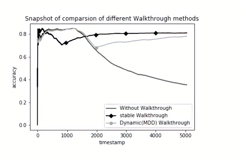
Figure 16 gives an overview of the comparison between the three different walkthrough
methods we tested.
For the first method, we train the deep learning model statically without walkthough, which
means we will not retrain or update the model when the accuracy decays. We can observe how
the accuracy drops significantly after roughly 1,500 predictions and reaches a value of less
than 40%, almost as low as random-guessing (25%), in the end.
When we use stable walkthrough to train our model, we will retrain at regular time periods.
Our tests are based on trading period or a financial trading cycle of five days. On our data,
this leads to four retrains (identified by rectangular points on the accuracy line). The first
retrain point has obvious effects in improving accuracy and it starts to go up slightly before
retraining. After four instances of retrain, the accuracy stabilizes around 80%.
When we use MDD-Dynamic Walkthrough method, we retrain the original model when
the accuracy drops by more than 15%. In our test, there is only one such instance (circle point
at around 2,000 mark). The accuracy has apparent growth after this model adjustment.
19Figure 16.: Snapshot of comparison between different walkthrough methods
Figure 17.: Comparison of different Walkthrough methods
We also perform the experiment for 20 times to compare the different walkthrough meth-
ods in order to have a stronger statistical guarantee; results are shown in Figure 17, (Consid-
ering that repeated experiments cost significant computation power and time, we repeat the
experiment 20 times to gather the results.) The results are in line with those discussed above,
i.e., stable walkthrough is better than the other two methods. The results also show that, for
dynamic (MDD) walkthrough method, only 2/3 retraining points occur in most experiments
(90%) while 2 experiments require 5 retraining points. But for stable walkthrough method,
all experiments need 4 retraining points. Therefore, when considering retrain time is a factor,
dynamic (MDD) walkthrough method is better because it needs less retraining in most cases.
The answer to RQ4 is multifold. Firstly, in multi-label prediction with deep learning
model, walkthrough training significantly improves the prediction accuracy. The reason is
that, as discussed above, deep learning prediction models need to update itself. When the
20model is not fit for the new market conditions, then it must be updated to achieve accu-
rate results. Secondly, stable walkthrough method is better than MDD-dynamic walkthrough
method, unless retrain time is important.
4. Validity of findings
The model is based on trading system; we select historical data and collect live data for
a long time span. The selection of data has no bias because historical trading contains all
available transaction data and available currency pairs in cryptocurrency market. Moreover,
the experiments are not affected by bull or bear market, policy impact and other factors. The
experiments use an extensive data selection, including bull-market condition, bear-market
condition, high-transaction-volume condition, low-transaction-volume condition etc.
Quality of data is another important factor to discuss. As the data is collected live from
Coinbase Pro, poor connection might affect the data (e.g., missing values). To mitigate this
risk, we have compared the data collected from Coinbase Pro with other third party service
providers to make sure the experiment have not been affected by inappropriate financial data.
5. Conclusions
This paper analyzes a data-driven approach to predict mid-price movements in cryptocurrency
markets, and covered a number of research questions en route regarding parameter settings,
design of neural networks and universality of the model. The main finding of our work is the
successful combination of an autoencoder and a walkthrough retraining method to overcome
the decay in predictive power on live data due to non-stationary features on the order book.
Prediction in high-frequency cryptocurrency markets is a challenging task because the envi-
ronment contains noisy information and is highly unpredictable. We believe that our results
can inform the design of higher level trading strategies and our networks architecture can be
used as a feature to another estimator.
References
Abergel, F. and Jedidi, A. (2015), ‘Long-time behavior of a hawkes process–based limit order book’,
SIAM Journal on Financial Mathematics 6(1), 1026–1043.
Adam, P. (2015), ‘Lstm implementation explained’.
URL: https://apaszke.github.io/lstm-explained.html
Ahamad, S., Nair, M. and Varghese, B. (2013), A survey on crypto currencies, in ‘4th International
Conference on Advances in Computer Science, AETACS’, Citeseer, pp. 42–48.
Altay, E. and Satman, M. H. (2005), ‘Stock market forecasting: artificial neural network and lin-
ear regression comparison in an emerging market’, Journal of Financial Management & Analysis
18(2), 18.
Biais, B., Hillion, P. and Spatt, C. S. (1995), ‘An empirical analysis of the limit order book and the
order flow in the paris bourse’, Journal of finance 50(5), 1655–1689.
Christopher, O. (2015), ‘Understanding lstm networks – colah’s blog’.
URL: http://colah.github.io/posts/2015-08-Understanding-LSTMs
Dixon, M. (2018), ‘Sequence classification of the limit order book using recurrent neural networks’, J.
Comput. Science 24, 277–286.
En.wikipedia.org (2018), ‘List of cryptocurrencies’.
URL: https://en.wikipedia.org/wiki/List of cryptocurrencies
21Fletcher, T. (2012), Machine learning for financial market prediction, PhD thesis, UCL (University
College London).
GDAX (2018), ‘Gdax api reference’.
URL: https://docs.gdax.com/#protocol-overview
Güresen, E., Kayakutlu, G. and Daim, T. U. (2011), ‘Using artificial neural network models in stock
market index prediction’, Expert Syst. Appl. 38(8), 10389–10397.
Hochreiter, S. and Schmidhuber, J. (1997), ‘Long short-term memory’, Neural computation
9(8), 1735–1780.
Huang, W., Nakamori, Y. and Wang, S.-Y. (2005), ‘Forecasting stock market movement direction with
support vector machine’, Computers and Operations Research 32(10), 2513–2522.
Kelly, F. and Yudovina, E. (2017), ‘A markov model of a limit order book: thresholds, recurrence, and
trading strategies’, Mathematics of Operations Research 43(1), 181–203.
Kercheval, A. and Zhang, Y. (2015), ‘Modelling high-frequency limit order book dynamics with sup-
port vector machines’, Quantitative Finance 15(8), 1315–1329.
Nakamoto, S. (2008), ‘Bitcoin: A peer-to-peer electronic cash system’.
Pro, C. (2018), ‘Global charts — coinmarketcap’.
URL: https://support.pro.coinbase.com/customer/en/portal/articles/2945310-fees
Sirignano, J. and Cont, R. (2018), ‘Universal features of price formation in financial markets: perspec-
tives from deep learning’.
Sundarapandian, V. (2009), Probability, statistics and queuing theory, PHI Learning Pvt. Ltd.
Tieleman, T. and Hinton, G. (2012), ‘Lecture 6.5-rmsprop: Divide the gradient by a running average of
its recent magnitude’, COURSERA: Neural networks for machine learning 4(2), 26–31.
Toke, I. M. and Pomponio, F. (2012), ‘Modelling trades-through in a limit order book using hawkes
processes’, Economics: The Open-Access, Open-Assessment E-Journal 6(2012-22), 1–23.
Tsantekidis, A., Passalis, N., Tefas, A., Kanniainen, J., Gabbouj, M. and Iosifidis, A. (n.d.), Using deep
learning to detect price change indications in financial markets, in ‘25th European Signal Processing
Conference (EUSIPCO)’, Vol. 4.
Wan, S. and Banta, L. E. (2006), ‘Parameter incremental learning algorithm for neural networks’, IEEE
Transactions on Neural Networks 17(6), 1424–1438.
Zhang, X., Li, A. and Pan, R. (2016), ‘Stock trend prediction based on a new status box method and
adaboost probabilistic support vector machine’, Appl. Soft Comput. 49, 385–398.
22You can also read