Estimation of Seqwater's productivity growth rate

Estimation of Seqwater’s productivity growth rate
A report prepared for Seqwater | 24 June 2021

Estimation of Seqwater’s productivity growth rate 2
 Final

Frontier Economics Pty Ltd is a member of the Frontier Economics network, and is headquartered
in Australia with a subsidiary company, Frontier Economics Pte Ltd in Singapore. Our fellow
network member, Frontier Economics Ltd, is headquartered in the United Kingdom. The
companies are independently owned, and legal commitments entered into by any one company
do not impose any obligations on other companies in the network. All views expressed in this
document are the views of Frontier Economics Pty Ltd.

Disclaimer
None of Frontier Economics Pty Ltd (including the directors and employees) make any
representation or warranty as to the accuracy or completeness of this report. Nor shall they have
any liability (whether arising from negligence or otherwise) for any representations (express or
implied) or information contained in, or for any omissions from, the report or any written or oral
communications transmitted in the course of the project.

Frontier Economics

Estimation of Seqwater’s productivity growth rate 3
 Final

Contents
1 Introduction 1
1.1 Background 1
1.2 Our instructions 1
1.3 Key findings 1
1.4 Structure of this report 3

2 Methods for estimating the productivity growth rate 4
2.1 Frontier shift versus catch-up 4
2.2 Key approaches for estimating productivity growth rate 6
2.3 Data availability 10
2.4 Conclusion 11

3 Estimating the productivity rate using data obtained from Seqwater 13
3.1 Introduction 13
3.2 Data used 13
3.3 Measures of inputs and outputs used 13
3.4 Results from PFP and TFP models 16
3.5 Conclusion 18

4 Estimating the productivity rate for bulk water supply using NPR data
 20
4.1 Introduction 20
4.2 Limitations of the NPR data 20
4.3 Measures of inputs and outputs used 20
4.4 Results from opex PFP indices 21
4.5 Conclusion 25

5 Productivity growth rate estimates for water distribution businesses 26
5.1 Introduction 26
5.2 Estimation approach used 26

Frontier Economics

Estimation of Seqwater’s productivity growth rate 4
 Final

5.3 Description of data used in the analysis 26
5.4 Measures of inputs and outputs used 27
5.5 Results from SFA models 27
5.6 Conclusion 30

6 Regulatory precedent 31
6.1 Introduction 31
6.2 Interpretation of recent regulatory precedent 32
6.3 Conclusions 36

7 Overall estimate of productivity 38

A Calculation of partial and total factor productivity indices 39
Tables
Table 1: Inputs used in the analysis 14

Table 2: Estimated annual growth rates in PFPs and TFP over different time periods 17

Table 3: Estimated productivity growth rates for bulk water supply businesses 24

Table 4: Estimated productivity growth rates for urban water distributors using SFA 30

Table 5: Regulatory decisions considered 31

Table 6: Regulatory precedent on the productivity growth rate considered by OTTER 35

Table 7: Summary of evidence 38

Figures
Figure 1: Summary of annual productivity growth rate estimates from different sources 2

Figure 2: Efficiency catch-up and frontier shift 5
Figure 3: Least squares (LS) and Corrected Ordinary Least Squares (COLS) 8

Figure 4: Stochastic frontier analysis (SFA) 9

Figure 5: Data envelopment analysis (DEA) 10

Figure 6: Inputs and outputs over time when the user cost of capital is used as the capital input
 16

Figure 7: PFP and TFP indices over time 17
Figure 8: Opex input indices for bulk water supply businesses 22

Figure 9: Output indices for bulk water supply businesses 23

Figure 10: Opex PFP for bulk water supply businesses 24
Figure 11: Indices using NPR data for Seqwater 25

Frontier Economics

Estimation of Seqwater’s productivity growth rate 5
 Final

Figure 12: Seqwater’s asset value compared to urban water distributors 28
Figure 13: Seqwater’s revenue compared to urban water distributors 29

Boxes
 : Törnqvist formula for change in aggregate input measure between periods s and t 40

 : Törnqvist formula for change in aggregate output measure between periods s and t 40

Frontier Economics

Estimation of Seqwater’s productivity growth rate Final

1 Introduction
1.1 Background

The Queensland Competition Authority (QCA) applies a base-step-trend approach to set Seqwater’s
operating expenditure (opex) allowances over a regulatory period. This involves:

• First establishing an efficient level of base year opex (in a selected base year);
• Making adjustments to that efficient base year level of opex to account for step changes in
 opex that are expected to occur over the regulatory period, which are not reflected in the base
 year level of opex; and

• Finally, trending the base year level of opex forward (accounting for expected changes in input
 costs, output growth and productivity) to develop a forecast of opex for each year of the
 forthcoming regulatory period.
In order to implement the ‘trend’ component of the base-step-trend approach, the QCA must make
a determination on the expected rate of productivity improvement in opex over the period.
In its regulatory proposal for the 2018-21 regulatory period, Seqwater proposed a cumulative
productivity growth rate of +0.2% p.a. KPMG, the QCA’s adviser during that price review on the
efficiency and prudency of Seqwater’s expenditures, considered that the productivity growth rate
proposed by Seqwater was low compared to the efficiency targets set by other regulators.
However, in its final report to the QCA, KPMG recommended that, in the absence of “more
sophisticated analysis of efficiency”, the QCA should adopt Seqwater’s proposed productivity
growth rate of +0.2% p.a.
The QCA accepted KPMG’s recommendation and noted KPMG’s advice that the QCA might
“consider undertaking further analysis before the next review using techniques such as total factor
productivity, stochastic frontier or data envelopment analysis.”1

1.2 Our instructions

We have been asked by Seqwater to develop an appropriate estimate of the productivity growth
rate for application in the QCA’s base-step-trend framework for setting opex allowances for its next
regulatory submission. Seqwater has asked us to have regard to the following, where feasible and
appropriate, when developing our estimate of an appropriate productivity growth rate:

• the techniques suggested by KPMG in its advice to the QCA; and
• recent regulatory precedent.

1.3 Key findings

In this report, we have:

1
 QCA, Seqwater Bulk Water Price Review 2018–21, Final Report, March 2018, p. 31.

Frontier Economics 1

Estimation of Seqwater’s productivity growth rate Final

• Considered the data available for developing empirical estimates of an appropriate
 productivity growth rate. These data include:
 o Information collected directly from Seqwater; and

 o Data compiled from the National Performance Review (NPR) dataset.

 We use data collected from Seqwater to derive Seqwater-specific estimates of the productivity
 growth rate. We concluded that the NPR data are not sufficiently reliable to derive robust
 estimates of the productivity growth rate for bulk water suppliers. However, the NPR data are
 sufficiently reliable and complete to derive productivity growth rate estimates for urban water
 distribution businesses (i.e., businesses in a closely-related industry to Seqwater’s).

• Considered the techniques that are feasible for developing estimates of the productivity
 growth rate, including:
 o Total Factor Productivity (TFP) analysis;

 o Stochastic Frontier Analysis (SFA); and

 o Data Envelopment Analysis (DEA).

 In this report, we use TFP analysis to derive productivity growth rate estimates for Seqwater
 and SFA to derive productivity growth rate estimates for water distribution businesses of
 similar scale to Seqwater. We conclude that there are insufficient data to estimate reliably the
 productivity growth rate for Seqwater or water distribution businesses using DEA.

• Considered the productivity growth rates applied in several regulatory decisions relating to
 water businesses between 2017 and 2020.
The estimates of the productivity growth rate using these different methods are summarised in
Figure 1 below.

Figure 1: Summary of annual productivity growth rate estimates from different sources

Source: Frontier Economics

Frontier Economics 2

Estimation of Seqwater’s productivity growth rate Final

Given this evidence, we consider that it would be reasonable for the QCA to apply an annual
cumulative productivity growth rate (reflecting frontier shift efficiency) of no higher than +0.2% p.a.
We note that this productivity growth rate would be consistent with the productivity growth rate
applied by the QCA to:

• Seqwater when setting its bulk water charges over the 2018-21 regulatory period; and
• Seqwater and Sunwater when setting prices relating to the supply of water for rural irrigation
 services.

1.4 Structure of this report

The remainder of this report is organised as follows:

• Section 2 provides an overview of the methods and approaches available for estimating the
 productivity growth rate, and the data available to us to undertake this task;

• Section 3 presents our estimates of the productivity growth rate for Seqwater using data
 obtained directly from Seqwater;

• Section 4 presents estimates of the productivity growth rate for major bulk water suppliers in
 Australia derived using the NPR dataset. We conclude that these estimates are not sufficiently
 reliable to inform an estimate of the productivity growth rate for Seqwater, due to severe
 limitations in the NPR data relating to bulk water suppliers;

• Section 5 presents estimates of the productivity growth rate for Australian water distribution
 businesses of a similar scale to Seqwater;

• Section 6 surveys and interprets the productivity growth rates applied in a sample of recent
 regulatory decisions; and

• Section 7 presents our overall conclusions, given the evidence compiled in this report, and
 provides our recommended productivity growth rate for Seqwater.

Frontier Economics 3

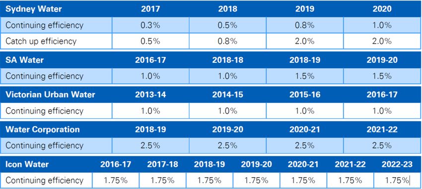
Estimation of Seqwater’s productivity growth rate Final

2 Methods for estimating the
productivity growth rate
2.1 Frontier shift versus catch-up

As explained in section 1, when applying a base-step-trend framework for determining the opex
allowance for a regulatory period, the QCA makes a determination on efficiency targets for the
regulated business. The efficiency target is often broken down into two separate components:

• A shift in the industry production frontier due to changes in technology, input costs,
 regulatory requirements and other cost drivers that affect all businesses in the industry. This
 ‘frontier shift’ is referred to as the productivity growth rate or “continuing efficiency”.

• Catch-up in efficiency, which refers to the improvements in efficiency that an inefficient
 business is expected to make to catch up to businesses on the efficient production frontier.
The QCA has itself recognised this distinction. For example, in its recent decision for the Gladstone
Area Water Board, the QCA explained that: 2

 Regulators typically apply two types of efficiency adjustments to controllable opex:

 • a catch-up efficiency—a firm-specific target to move a business closer to the efficient
 frontier (typically measured as the best performing comparable businesses)

 • a continuing efficiency—an industry-wide target reflecting the movement of the efficient
 frontier over time as productivity improves, for example, due to innovation.

These two aspects of the efficiency target are illustrated in Figure 2. The Figure shows the efficient
opex cost frontiers for two years, year 1 and year 2. The cost frontier in year 2 is lower than in year
1 due to improvements in productivity. This is referred to as frontier shift.
If, in year 1, a business had output at Y and opex at A, then its opex would be larger than the
efficient level of opex for an output of Y (shown as B). For the business to reach the opex frontier
in year 1 it would have to reduce its opex in year 1 from A to B in order to “catch up” with the
efficient frontier.
A business with output Y in year 1 and opex at B is efficient in year 1 since it is operating on the
efficient opex frontier. If output doesn’t change between years 1 and 2, then in order to stay
efficient in year 2, the business will have to reduce its opex to C to keep up with the downward
“frontier shift” for opex due to productivity improvements.

2
 QCA, Gladstone Area Water Board price monitoring 2020–25 Part A: Overview, Final Report, May 2020, p. 43.

Frontier Economics 4

Estimation of Seqwater’s productivity growth rate Final

Figure 2: Efficiency catch-up and frontier shift

Source: Frontier Economics

In the base-step-trend regulatory framework, the catch-up element of efficiency improvement is
considered when determining the level of efficient opex in the base year for the regulatory period.
The frontier shift component (or the “continuing efficiency” factor, as the QCA refers to it) is
accounted for in the trend term. In this report we focus on this second aspect of the efficiency
target, namely, the shift in the efficient production frontier over the forthcoming regulatory period
(i.e., frontier shift).
A forecast of frontier shift during the upcoming regulatory period may be informed by an estimate
of the historical change in productivity. However, the ability to estimate the historical rate of
productivity accurately is typically limited by:

• Incomplete historical data;
• Uncertainty over how the inputs and outputs of the business are to be measured;
• The ability to control properly for factors unrelated to productivity changes that could
 influence a business’s inputs and outputs; and

• The shortcomings of the models available to estimate the historical rate of productivity (noting
 that there are many different techniques for estimating the historical rate of productivity, each
 with their own strengths and weaknesses).
Furthermore, it is important to recognise that the historical change in productivity may not be
reflective of what is achievable or realistic over the forthcoming regulatory period for two main
reasons:

• The estimated historical rate of productivity change may include an element of catch-up as
 well as a shift in the cost frontier. In practice, it can be challenging to separate these two

Frontier Economics 5

Estimation of Seqwater’s productivity growth rate Final

 effects using the standard techniques and models available for measuring the historical rate
 of productivity. The forecast of the productivity growth rate should only reflect expected
 frontier shift, and should exclude any contribution to historical estimates of productivity
 growth due to catch-up. Conflating the two is likely to result in the achievable future
 productivity growth rate being overstated. This would result in the business receiving an opex
 allowance that is lower than the efficient level.

• The impact on opex of changes in technology and other cost drivers over the forthcoming
 regulatory period may not be the same as over the historical period used to estimate the past
 change in productivity.
This means that even if one could estimate the historical productivity growth rate with complete
certainty (which is generally not possible, for the reasons explained above), there may be still be
uncertainty over the extent of continuing efficiency achievable by a regulated business over a
future regulatory period. Therefore, a considerable degree of caution and judgment is required
when determining the continuing efficiency targets that are to be imposed on a regulated business
when setting its expenditure allowances for a future regulatory period.

2.2 Key approaches for estimating productivity growth rate

There are three main approaches to estimating the productivity growth rate:

• Approaches based on index numbers, which can be split in Total Factor Productivity (TFP) and
 Partial Factor Productivity (PFP)

• Econometric approaches – one of the most common being Stochastic Frontier Analysis (SFA);
 and

• Data envelopment analysis (DEA).
The QCA has indicated that it may consider these three approaches as part of its review process.3
We discuss each of these in turn.

2.2.1 Index based approaches

Index based approaches to productivity measurement take an index of a measure of output and
divide it by an index of a measure of input. Changes in this ratio over time provide a measure of
the change in productivity over time.4 If the measure of output is an aggregate measure that
captures the levels of all outputs produced by a business, and the measure of input is an aggregate
measure of the levels of all the inputs used by that business to produce those outputs, then the
index is referred as a total factor productivity (TFP) index.
Examples of outputs often considered for water utilities are the volume of water delivered,
customer numbers and network size. Examples of inputs are opex and capital. Both opex and the
capital input may be broken down further into sub-categories, e.g. labour, chemicals and energy,
or water treatment plants and pipes.

3
 “However, the QCA may consider undertaking further analysis before the next review using techniques such as
 total factor productivity, stochastic frontier or data envelopment analysis.” QCA (2018), Seqwater Bulk Water Price
 Review 2018–21, p.31.
4
 The approach can also be applied to several businesses at the same point of time (cross-sectional productivity
 comparisons), or several businesses across time (multilateral productivity comparisons).

Frontier Economics 6

Estimation of Seqwater’s productivity growth rate Final

The rate of change in the TFP index is a measure of the total productivity growth factor. This can
provide information on performance from one year to the next, and when averaged over a number
of years, it provides an indication of longer-term growth in productivity. We note, however, that
changes in TFP capture the combined effect of catch-up in efficiency and the shift in the frontier
function. Nevertheless, while there are no formal methods for separating these two aspect of a
change in productivity, by inspecting the year to year changes in the TFP index, one may be able to
identify periods when catch-up seems to dominate the change in TFP versus periods where frontier
shift is more likely to be the driving factor.
It is also possible to construct a range of partial factor productivity (PFP) indices. The most common
examples are the PFP index for opex and the PFP index for capital input. In each of these cases,
the numerator of the index ratio is the aggregate measure for total output, while the denominator
is either opex or a measure of capital input. These PFPs provide an indication of the productivity
of the business in terms of opex spending or the use of capital.
We note that TFP and PFP analysis can be performed for an individual firm or for a number of firms
collectively, e.g., the industry as a whole. It is also worth noting that when combining different
outputs into a single output measure, or different inputs into a single input measure, it is necessary
to use appropriate weights. There are a number of different approaches to calculating these
weights. The most commonly used approach is a method known as the Törnqvist Index. This is the
approach we have adopted in this report.

2.2.2 Econometric methods

There are several econometric techniques that are used by regulators to undertake benchmarking
analysis, for example:

• Least Squares estimation of an average cost function;
• Corrected Ordinary Least Squares (COLS);
• Least Squares panel estimation with fixed effects (FE) or random effects (RE); and
• Stochastic Frontier Analysis (SFA).
All these methods involve essentially the same idea:

• Assume that costs are a function of one or more cost drivers and a time trend to capture
 changes in productivity over time:

(1) = + + + + 

• Estimate this econometric relationship between costs and cost drivers
• Use the fitted relationship to define an efficient frontier or reference cost function
• Interpret the distance between the firm in question and the fitted frontier/reference function
 as an estimate of efficiency. In the case of SFA, allowance is also made for random statistical
 noise in the differences between the firm in question and the estimated efficiency frontier.
The estimated coefficient on the time trend can be interpreted as an estimate of the productivity
growth rate. However, we note that, as with any statistical analysis, estimates of efficiency and the
productivity growth rate will only be reliable if all relevant cost drivers are accounted for properly
in the model, and if the data used in the analysis are reliable.

Frontier Economics 7

Estimation of Seqwater’s productivity growth rate Final

Least squares (LS) and Corrected Ordinary Least Squares (COLS)

Figure 3 illustrates the first two of the above approaches. The least squares (average) cost function
is indicated by the solid line in the chart. Based on a sample of observations (which could be a
single business over a period of time, or several businesses at the same point in time, or a
combination) it shows the estimated average opex used in the sample to produce different levels
of output. We have drawn this average cost line as a straight line, but in practice non-linear
functions are often used to fit the relationship between costs and cost drivers.
By comparing the opex of individual observations with the average cost line, one can determine
whether a business is using more or less opex than the average business would use to produce
the same level of output.
The Corrected Ordinary Least Squares (COLS) function is obtained from the average cost line by
shifting the average cost line down in a parallel fashion until there are no points below the line,
and there is one point (or several points) exactly on the line. This is illustrated in Figure 3 by the
dashed line. The businesses on the dashed line are regarded as being efficient. For other
observations, the vertical distance between the point and the dashed line is a measure of the
business’ inefficiency.

Figure 3: Least squares (LS) and Corrected Ordinary Least Squares (COLS)

Source: Frontier Economics

If panel data are available, that is, data on several businesses over a number of years, then variants
of the COLS approach can be estimated. In this approach, each business is assumed to have an
efficiency factor that is constant over time, that can be represented by either a fixed effects or
random effects approach. Rather than evaluating the efficiency of each individual observation
relative to the frontier or average cost function, this approach produces estimates of each
business’ average efficiency over the sample period relative to the most efficient business.

Frontier Economics 8

Estimation of Seqwater’s productivity growth rate Final

Stochastic frontier analysis (SFA)

Stochastic frontier analysis (SFA) is a more sophisticated econometric approach to estimating
efficiency. Instead of interpreting the residual term in equation (1) above as representing only
inefficiency, this term is now interpreted as a combination of an inefficiency component as well as
random noise. This is illustrated in Figure 4 below. Note that because allowance is made for a
random noise term in the model, it is possible that some observations lie slightly below the frontier
cost line.
Estimating a model that decomposes the residual term in this way requires additional statistical
assumptions and a more advanced estimation technique than least squares estimation. It also
requires a larger sample to achieve reliable results. However, if the assumptions underlying the
model are satisfied, the estimates of the inefficiency terms and the productivity growth rate are
likely to be more precise than when using the least squares and COLS methods.
The Australian Energy Regulator (AER) has relied on SFA models in its recent regulatory reviews for
electricity distribution utilities. SFA studies for urban water distribution utilities have also been
undertaken on behalf of the Essential Services Commission of Victoria (ESC).

Figure 4: Stochastic frontier analysis (SFA)

Source: Frontier Economics

2.2.3 Data envelopment analysis (DEA)

Another technique widely used for benchmarking is data envelopment analysis (DEA). This is a non-
parametric technique in that it does not specify a particular functional form for the relationship
between cost and the cost drivers. Instead it uses linear programming to fit a piece-wise linear
envelope to the data to derive the efficient frontier, as illustrated in Figure 5. Any business whose

Frontier Economics 9

Estimation of Seqwater’s productivity growth rate Final

cost is higher than the efficient frontier is considered to be inefficient. The DEA technique does not
make any allowance for random noise in the data.
If DEA is applied over time, the shift in the frontier over time can be used to estimate the rate of
productivity growth. However, this requires a considerable amount of data since separate frontiers
need to be estimated for each point in time.

Figure 5: Data envelopment analysis (DEA)

Source: Frontier Economics

2.3 Data availability

The analysis in this report has relied on the following data sources:

• The National Performance Report (NPR) database produced by the Bureau of Meteorology; 5
• Information provided directly by Seqwater; and
• Information contained in QCA determinations for Seqwater.
The NPR database provides data on Australian water utilities, including bulk water providers and
water distribution networks, which is a closely related industry. The most recent release of the data
was used, which provides data up to and including the 2019-20 financial year, and going as far back
as 2002-03 for some utilities/variables.

5
 Bureau of Meteorology, National Performance Report database, available at
 http://www.bom.gov.au/water/npr/docs/The_complete_dataset_2019_20.xlsx

Frontier Economics 10

Estimation of Seqwater’s productivity growth rate Final

While the NPR database does provide opex data for bulk water utilities, there are significant gaps
in this dataset. For WaterNSW there are no opex data for 2015-16 through 2017-18, and for
Seqwater opex data are missing for 2014-15 and 2016-17. Moreover, the opex for Seqwater in
2015-16 is reported as $821,190, which is implausibly low. The opex data provided is the total
across all cost categories – there is no decomposition into different cost categories such as labour
or electricity.
In view of this, we requested more detailed data from Seqwater. The data we were provided
covered the period 2014 to 2019 and contained information on the quantity and cost of a range of
inputs, as well as on several outputs.
While we were able to collect data directly from Seqwater, given the timeframe available to prepare
this report and likely challenges in gaining cooperation from the businesses, we did not consider
it feasible to collect data directly from the other bulk water providers.

2.4 Conclusion

In light of the data available to us and the data requirements of different methodological
approaches, we concluded that it would be feasible to undertake the following quantitative
analyses to obtain estimates of the rate of growth in productivity:

• Calculate the TFP and opex PFP indices for Seqwater using data obtained directly from
 Seqwater. These indices would provide an indication of Seqwater’s total factor productivity
 and opex productivity over time. Changes in historical productivity from one year to the next
 and the average rate of productivity over a number of historical years can be estimated using
 these indices.

• Use the NPR dataset to calculate the opex PFP index for the major bulk water suppliers
 captured in the NPR dataset (Seqwater, Melbourne Water, WaterNSW, SA Water and Water
 Corp). This would potentially provide a comparison of the rate of productivity over time of
 Australian businesses whose operations are very similar to those of Seqwater. As explained in
 section 4.3, we were unable to construct TFP indices for bulk water suppliers using the NPR
 dataset since the NPR dataset does not contain the information on capital inputs that we
 required to implement such an approach. We also concluded that the sample of bulk water
 supply businesses is too small to reliably estimate an SFA model or any other econometric
 model.

• Estimate an SFA model for urban water distribution businesses using the NPR dataset. This
 would provide an estimate of average productivity growth over the sample period in an
 industry that is closely related to bulk water supply, with similar cost drivers. We chose SFA
 over other econometric approaches because SFA enables operational inefficiency to be
 considered separately from random noise, and because the QCA has previously indicated its
 intention to consider relevant SFA evidence. We also considered that the sample of urban
 water distribution businesses in the NRP dataset is large enough to make SFA feasible. 6
We did consider the DEA approach to estimate the productivity growth rate for the urban
distribution businesses. However, we concluded that DEA modelling would present technical
challenges, as it would require estimation of separate efficient frontiers for each historical year in

6
 While the NPR data for the water distribution businesses also has some quality issues, given there is a much
 larger sample of distribution businesses than bulk supply businesses, and the fact that the SFA model allows for
 random errors in the data, data quality issues will have much less impact on the results for the distribution
 businesses than for the bulk supply businesses.

Frontier Economics 11

Estimation of Seqwater’s productivity growth rate Final

the dataset. The productivity growth rate would then need to be estimated by analysing the change
in the efficient frontier between years. However, due to gaps in the dataset, the frontiers for
different years would be based on samples of different sizes and comprised of different
businesses. Hence the efficient frontiers in different years would not be comparable. 7 This would,
in our view, make the estimate of the productivity growth rate using DEA unreliable.

7
 For a discussion of the difficulties in comparing the results of separate DEA analyses carried out on samples of
 different sizes see Zhang, Y. and Bartels, R. (1998), "The effect of sample size on the mean efficiency in DEA with
 an application to electricity distribution in Australia, Sweden and New Zealand", Journal of Productivity Analysis, 9,
 187-204.

Frontier Economics 12

Estimation of Seqwater’s productivity growth rate Final

3 Estimating the productivity rate
using data obtained from Seqwater
3.1 Introduction

Our first approach to estimating the productivity growth rate for Seqwater is to undertake an
analysis of the historical growth rates in Seqwater’s partial productivity indices (PFPs) and the total
factor productivity index (TFP). While efficiency and productivity studies frequently focus on a
business’ operating expenditure, in our view it is helpful to also consider productivity in the use of
capital, since the possibility of substitution between opex and capex can distort estimates of
productivity changes with respect to either one of these inputs. Hence, in this section we present
estimates not just of the partial productivity factor (PFP) for opex, but also the PFP for capital and
the total factor productivity (TFP).

3.2 Data used

As outlined in section 2.3, for this task we relied on data provided by Seqwater. We did not use the
NPR dataset for this task because it did not provide any disaggregated detail on opex, there were
considerable gaps in the data, and some of the data seemed less reliable than the data provided
by Seqwater.
To calculate the PFP and TFP indices, we need both the physical quantities of inputs used, and the
expenditures on those inputs.8 For some of the inputs we did not have the physical quantities of
the inputs or the quantity data seemed unreliable (for example, for some of the chemicals used).
For each of those inputs, we proxied the quantity of the input by the deflated series of expenditures
for the input. The cost deflators we used for this purpose were chosen to be consistent with the
QCA’s approach and Seqwater’s cost escalation approach.
Seqwater was unable to provide us with data for FY2020 within the timeframes available to prepare
this report. We chose not to supplement the data provided by Seqwater with FY2020 NPR data for
Seqwater since the results would be sensitive to differences between methodologies for
constructing the two datasets. Furthermore, due to our reservations about the reliability of the
NPR data for Seqwater in historical years, we considered that it would be imprudent to use the
FY2020 NPR data for Seqwater. As a consequence, we relied only on the data provided to us by
Seqwater data up to and including FY2019.

3.3 Measures of inputs and outputs used

Outputs

We requested and were provided with information on a number of outputs produced by Seqwater.
In addition to the total volume of urban water supplied we considered the volume of irrigation
water supplied, water quality measures, and water security measures. The data for the volume of

8
 The expenditures are needed to calculate the expenditure shares of the different inputs, which are used as
 weights in the Törnqvist index formula.

Frontier Economics 13

Estimation of Seqwater’s productivity growth rate Final

irrigation water was not closely correlated with opex, hence we excluded it from out consideration.
We also excluded the water quality measures on the basis that they typically took only a few distinct
values, and they were not considered to be major cost drivers. Water security measures, such as
storage levels, were considered to be more reflective of drought conditions rather than a driver of
costs. Hence, we selected the total volume of urban water supplied as the most relevant output
for our analysis. This is also one of the main cost drivers typically considered in the analysis of
water distribution productivity. The use of a single output variable also reduces the complexity of
calculating the productivity indices, since it circumvents the need to derive output weights required
when combining several output variables into a single measure of output.
Operating expenditures

We requested and were provided with detailed expenditure information for Seqwater. We
combined the opex expenditures into seven categories, with expenditure information covering the
period from FY2014 to FY2019. These are shown in the first seven rows of Table 1

Table 1: Inputs used in the analysis

 Input category Measure of input used in analysis

 Electricity Electricity: actual quantities (MWHr)

 Chemicals Chemicals: cost deflated using Brisbane CPI

 Sludge disposal Sludge disposal: actual quantities (Tonnes)

 Maintenance Maintenance: cost deflated using Brisbane CPI

 Labour Labour: actual quantities (FTEs)

 Contractors: cost deflated using 56% QLD WPI,
 Contractors
 44% Brisbane CPI

 Other Other: cost deflated using Brisbane CPI

 Capital costs (for TFP and capital cost PFP) Capital costs: cost deflated using Brisbane CPI

Source: Frontier Economics

Note: The cost deflators were chosen to be consistent with QCA’s approach and Seqwater’s cost escalation approach

The calculation of the PFP and TFP indices requires data on the physical quantities used in each
input category. For several of the inputs we did not have data on the physical quantities or the data
seemed unreliable. For those inputs we used the deflated expenditures for that category as a proxy
for the quantity of input.
The cost deflators we used for each input are shown in the second column of Table 1. We deflated
chemicals, maintenance and other costs using the Brisbane CPI.9 This is consistent with the
approach used in the 2018 Decision. 10,11 Contractor expenses are deflated using a weighted

9
 ABS 6401.0, series A2325816R.
10
 QCA, 2018 Final Report, p. 15.
11
 QCA, 2018 Final Report, p. 54.

Frontier Economics 14

Estimation of Seqwater’s productivity growth rate Final

combination of the Queensland wage price index12 and the Brisbane CPI as proposed by Seqwater
for the 2018 review and accepted by the QCA.13
Capital input

In principle, the capital input used in productivity analysis should reflect the flow of capital used in
production, analogous to the hours of labour used or the quantity of chemicals, rather than the
stock of assets. When the stock of assets is used as the capital input, there is an implicit assumption
that the flow of capital stock used in production is proportional to the stock of capital.
In this study, we have used the ‘user cost of capital’ approach to measure capital inputs. The
traditional approach to calculating the annual user cost of capital is to take the sum of the nominal
return on capital and nominal depreciation, and subtract capital gains. We adopted an ex ante
approach to this task, whereby the returns on and of capital for FY2014 through FY2018 were taken
from the 2015 Decision,14 and the return on and of capital for FY2019 were taken from the 2018
Decision.15 In the 2015 Final Report, the inflationary gain in the RAB was deducted from the figures
for the return on capital. In the 2018 Final Report, an indexation amount for inflation was reported
separately; we subtracted this from the return on capital.
To obtain a time series of the user cost of capital in constant dollar terms for the capital input into
production, we deflated the user cost of capital values using the Brisbane CPI.
Taking an ex ante approach means that we are using the QCA’s assessment of the anticipated
efficient user cost of capital over the regulatory period. This is consistent with our aim of estimating
the shift in the efficient frontier rather than a combination of frontier shift and catch-up.
Figure 6 below shows the inputs used in our analysis over time. The chart shows that opex inputs
decreased through to FY2017, thereafter increasing and returning to FY2014 levels in FY2019. The
reduction to FY2015 was driven by reductions in maintenance, contractors and the ‘other
materials/inputs’ category; the increase between FY2017 and FY2018 was driven by growth in
labour, contractors and the ‘other materials/inputs’ category.
Capital input, as measured by the user cost of capital, increased steadily over the period, with the
exception of an abnormally high user cost of capital in FY2015. This was driven by a low inflation
forecast for FY2015 at the time the QCA made its determination. This meant that a relatively
modest amount of expected inflation was subtracted by the QCA from the allowed return on assets
for FY2015.
A comparison between the output index and the total input index suggests that, overall, inputs
increased in line with the output, measured by the total volume of urban water supplied. However,
the capital input grew considerably faster than output, while opex declined slightly over the period.
This suggests that over the sample period there may have been substitution away from opex
towards capital.

12
 ABS 6345.02a, series A85021977A.
13
 PWC, Cost escalation factors – Final report, July 2017, p. 23.
14
 QCA, 2015 Final Report, Table 26.
15
 QCA, 2018 Final Report, Table 57.

Frontier Economics 15

Estimation of Seqwater’s productivity growth rate Final

Figure 6: Inputs and outputs over time when the user cost of capital is used as the capital input

Source: Frontier Economics analysis of data supplied by Seqwater

3.4 Results from PFP and TFP models

The technical Appendix to this report explains how we construct the PFP and TFP indices.
The results from the PFP and TFP analysis are shown in Figure 7. The Figure shows that opex
productivity (represented by the opex PFP index) increased between FY2014 and FY2017, after
which it declined slightly between FY2017 and FY2018, and has remained flat between FY2018 and
FY2019. In its 2018 review the QCA reported that: 16

 KPMG noted that actual expenditure has been consistently below that recommended by
 the QCA in the 2015 review, lending support to the contention that Seqwater has achieved
 efficiencies over the regulatory period

Figure 7 suggests that these efficiencies were achieved as a result of catch-up to the frontier in the
years up to 2017. Catch-up in efficiency cannot be sustained over the longer period. Once a
business has caught up with the frontier, future efficiency gains can only be expected to occur as
a result of frontier shift.

16
 QCA (2018), Seqwater Bulk Water Price Review 2018–21, p.21.

Frontier Economics 16

Estimation of Seqwater’s productivity growth rate Final

It is likely that the changes in opex productivity that we observe after 2017 are due to frontier shift
rather than catch-up. One can expect future changes in productivity to be similar to the changes
after 2017 rather than those up to 2017.
Figure 7 shows that over the whole period from 2014 to 2019, opex productivity increased at an
annual rate of 2.2%. However, this estimate of productivity growth is very sensitive to the years
used to calculate the growth rate. While opex productivity exhibits high growth over 2014-2016,
the annual growth rates in opex productivity from 2016 or 2017 onwards, when catch-up in
efficiency might be assumed to have been achieved, are negative. The growth rates in opex
productivity over the different periods are summarised in Table 2.

Figure 7: PFP and TFP indices over time

Source: Frontier Economics analysis of data supplied by Seqwater

Table 2: Estimated annual growth rates in PFPs and TFP over different time periods

 Annual growth in Annual growth in Annual growth in
 Period
 opex PFP capital PFP TFP

 2014 - 2019 +2.2% -2.2% -0.7%

 2014 - 2017 +6.0% -4.3% -1.0%

 2017 - 2019 -3.2% +0.9% -0.4%

Source: Frontier Economics analysis of data provided by Seqwater

Frontier Economics 17

Estimation of Seqwater’s productivity growth rate Final

The chart also shows that there was a considerable fall in capital productivity between 2014 and
2015 of over 20%, with a partial rebound the following year, after which the capital PFP has
remained almost flat. The growth rates in capital productivity over the different periods are
summarised above in Table 2.
It is possible that the gain in opex productivity in the earlier years was due to substitution between
opex and capital expenditure. The ACCC notes that: 17

 For cost-benchmarking applications, it is important to ensure that there are no artificial
 incentives that create cost inefficiency through. . . substitution of capital expenditure for
 operating expenditure.

Such substitution of non-capital inputs for capital inputs is likely to have improved the overall
efficiency of the firm. However, the improvement in productivity may be overstated if one were to
focus only on the change in productivity of the non-capital investments. For example, the firm may
have invested in new technology that results in a reduction in its labour force (and, therefore, its
opex). This would manifest as (a potentially large) increase in the opex PFP, but a reduction in the
capital PFP—since the firm has substituted some non-capital inputs for additional capital inputs.
The net effect of this substitution may be that, overall, the firm has become somewhat more
productive. However, focussing exclusively on the opex PFP may create the false impression that
the overall productivity of the firm has increased very substantially.
To reduce the risk of drawing erroneous conclusions of this nature, it is desirable to consider not
only partial productivity measures, but also the firm’s total factor productivity. The TFP index in
Figure 7 shows that the TFP index, like the capital PFP index, decreased between 2014 and 2015,
with a rebound the following year. The changes in the TFP index are similar to those of the capital
PFP, but the swings are less severe due to the impact of the rise in the opex PFP between 2014 and
2017.
Over the whole period from 2014 to 2019, TFP changed by -0.7% p.a. As shown Table 2, the average
annual growth rate in TFP from 2017 onwards (i.e., the period after significant catch-up in efficiency
appears to have been achieved by Seqwater) is -0.4% per year.

3.5 Conclusion

We found that over the period 2014 to 2019, the average annual growth in Seqwater’s partial and
total productivity measures are:

• +2.2% p.a. for the opex PFP;
• -2.2% p.a. for the capital PFP; and
• -0.7% p.a. for TFP.
However, it seems likely that the growth in Seqwater’s opex PFP over some of this period may be
attributable to catch-up efficiency rather than frontier shift alone. Indeed, in its 2018 final decision

17
 ACCC (2012), Benchmarking Opex and Capex in Energy Networks, ACCC/AER Working Paper Series, Working Paper
 no.6, p.21.

Frontier Economics 18

Estimation of Seqwater’s productivity growth rate Final

for Seqwater, the QCA noted that Seqwater had made significant and consistent efficiency
improvements in opex over the previous regulatory period.
Catch-up efficiencies cannot be realised indefinitely. Once a firm has caught up to the efficient
frontier, future efficiencies can only be realised through frontier shift. Seqwater’s opex PFP shows
a significant increase between 2014 and 2017. It is likely that the changes in opex productivity that
we observe after 2017 are due to frontier shift rather than catch-up. To investigate this possibility
we estimated the same three productivity measures over the period 2017 to 2019.18
Our analysis shows that over the period 2017 to 2019, Seqwater’s partial and total productivity
measures are:
• -3.2% p.a. for the opex PFP;

• +0.9% p.a. for the capital PFP; and
• -0.4% p.a. for TFP.
One can expect future changes in productivity to be similar to the changes after 2017 rather than
those up to 2017.
We have computed a TFP measure for Seqwater as well as opex and capital PFPs. It is well-
recognised in the literature, and by economic regulators, that firms may substitute efficiently
between capital and non-capital inputs to production. Movements in a firm’s opex PFP may (in part)
reflect such substitution choices. For instance, a firm may elect to undertake more maintenance
work to extend the life of its assets and avoid expensive asset replacement. This would result in a
reduction in the firm’s opex PFP and an improvement in the firm’s capital PFP (all else remaining
equal). The opposite may also be true. A firm may favour capital expenditure solutions over opex
solutions (e.g., the investment in new technology to free up labour), and such choices may also be
efficient. In such circumstances, the firm’s opex PFP would increase, and its capex PFP would
decline (all else remaining equal). The overall productivity of the firm’s production choices can be
seen by examining changes in its TFP over time.
We therefore recommend that the QCA have regard to TFP results when determining an
appropriate productivity growth rate for Seqwater to avoid the estimates of the productivity
growth rate being confounded or distorted by such input substitution choices. Seqwater’s average
historical productivity growth rate, measured using a TFP index, ranges between -0.7% p.a. and
-0.4% p.a., depending on the historical period considered.

18
 See Table 2.

Frontier Economics 19

Estimation of Seqwater’s productivity growth rate Final

4 Estimating the productivity rate for
bulk water supply using NPR data
4.1 Introduction

We also investigated whether an appropriate productivity growth rate for Seqwater could be
estimated using the opex productivity growth rate for each of the five bulk water supply utilities
included in the NPR database – Seqwater, Melbourne Water, WaterNSW, SA Water, and Water
Corporation (Perth).19 Our aim was to obtain a range of opex productivity growth rates across
businesses in the bulk water supply industry to inform our assessment of what productivity growth
rate might be reasonable to expect Seqwater to achieve over the upcoming regulatory period. The
success of this approach depends, of course, to a large extent on the quality of data available for
this task. Hence, we first discuss the limitations of the NPR dataset with respect to the bulk water
supply businesses.

4.2 Limitations of the NPR data

As noted previously, there are substantial deficiencies in the NPR database. There are gaps for key
variables, for example operating costs of WaterNSW. We observed that in some years, operating
costs for water supply20 were not reported, yet operating costs per ML of water supplied was
reported, which enabled the derivation of operating cost for that year. 21
We also sought to remove the desalination costs of Melbourne Water that were submitted as a
component of the operating cost in the NPR database from FY2013 onwards, as the delivery of
desalination services is unrelated to the regulated bulk water services delivered by Seqwater. It is
our understanding that these costs were not only operating costs associated with the desalination
plants, but included a substantial amount of lease payments. After receiving advice from
Melbourne Water, we removed these payments by subtracting the amounts reported in
Melbourne Water’s published annual accounts. The desalination volumes were not included in the
water supply volume measure used for Melbourne Water.
While we use Seqwater supplied data for Seqwater for this task,22 we also present results using
NPR data for Seqwater, to illustrate the impact of using NPR data on any findings.

4.3 Measures of inputs and outputs used

As in section 3, we used the volume of water supplied as the sole output measure for bulk water
utilities. To obtain the volume of water supplied we took the maximum of three measures:

19
 We did not calculate the TFP growth rates for this investigation because of data limitations.
20
 NPR dataset variable IF11.
21
 For example, if we observe operating cost per ML, revenue per ML and revenue, we can infer the operating cost
 indirectly.
22
 We use Seqwater data from FY2014 through to FY2019 as we were unable to obtain FY2020 data within the
 timeframes available to prepare this report.

Frontier Economics 20

Estimation of Seqwater’s productivity growth rate Final

• The sum of surface water, ground water and desalination volumes;
• Total volume of urban water supplied (W11); and
• Volume of potable water produced for supply into the urban water system (W11.3).
As disaggregated cost information is not available in the NPR database, we used the water supply
operating cost as the sole input measure. 23 Nominal operating cost was deflated using an equally
weighted combination of the appropriate capital city wage price index and consumer price index.24
We also observed several anomalies with the NPR data:

• No desalination volumes were reported for Water Corporation (Perth) in FY2014, though it is
 our understanding that desalination volumes were being produced during FY2014.

• WaterNSW reported a large (85%) increase in operating cost between FY2015 and FY2019,
 though operating cost per ML declined considerably.

• Seqwater reported implausibly low operating costs in FY2016.
As the NPR data for Seqwater, in particular the operating cost information, are unreliable, we used
the Seqwater supplied data rather than data sourced from the NPR database for Seqwater.
However, for the other four bulk water suppliers we currently had no viable alternative to the NPR
database. Therefore, the results presented below use NPR data for Melbourne Water, WaterNSW,
SA Water, and Water Corporation (Perth).
As the NPR database does not contain data on the user cost of capital, we are unable to repeat the
TFP analysis applied to Seqwater in section 3 using NPR data. While the NPR dataset does contain
information on written down asset values, this is not in our opinion an ideal measure of capital
cost.

4.4 Results from opex PFP indices

As noted in the previous section, to calculate the opex PFP indices for the five bulk water supply
businesses, we used opex as the input measure and the volume of water supplied as the output
measure. While it would have been desirable to use more disaggregated measures of inputs
and/or outputs, that approach was not feasible due to the limitations of the NPR dataset.
Figure 8 and Figure 9 show the input and output indices for each of the five bulk water supply
businesses over time. Note in Figure 8 that, for WaterNSW, opex data were only available for 2014,
2015, 2019 and 2020, and that there was a very material increase in real opex of almost 80%
between 2015 and FY2019, from $99 million to $180 million (real $2014). This increase was
anomalous, with a substantial decrease in FY2020 to $99 million (real $2014).
Real opex for SA Water, on the other hand, decreased substantially over the period, falling by 18%
from $368 million to $302 million (real $2014).
The trends in opex over the sample period for the other three businesses fall between these two
extremes.

23
 This includes water distribution expenses for SA Water and Water Corporation – Perth.
24
 We follow the approach of Economic Insights’ 2017 Victorian urban water utility benchmarking report for the
 Essential Services Commission of using a simple (equal-weighed) average of wage and consumer price indices.

Frontier Economics 21

Estimation of Seqwater’s productivity growth rate Final

Figure 8: Opex input indices for bulk water supply businesses

Source: Frontier Economics analysis of NPR data and data supplied by businesses

The output indices in Figure 9 show slightly increasing trends for Seqwater, Melbourne Water and
SA Water over the period. For WaterNSW, output increased moderately between 2014 and 2016,
and then decreased quite sharply over the following years.
Output for Water Corporation (Perth) is affected by a change in reporting practices. In 2014, water
produced by desalination was not included as part of the output volume for that year, whereas in
subsequent years it was included. In view of this, we have calculated two opex productivity growth
rates for Water Corporation (Perth), one for the whole sample period and the other for the period
from 2015 to 2020. We also note that in 2018 there was a large increase in storage levels, which
likely explains the large increase in output in the last two years.
For the other three businesses, output increased slightly between 2014 and 2020 with relatively
little volatility from year to year.

Frontier Economics 22

Estimation of Seqwater’s productivity growth rate Final

Figure 9: Output indices for bulk water supply businesses

Source: Frontier Economics analysis of NPR data and data supplied by businesses

Combining the input and output indices results in the opex PFP indices shown in Figure 10 and
summarised in Table 3. The estimated productivity growth rates vary widely between businesses.
The largest estimated productivity growth rate is for Water Corporation (Perth) over the whole
sample at 12.63% p.a. If data for 2014 are excluded, because of the change in the way desalination
volumes are accounted for, the productivity growth rate for Water Corporation (Perth) reduces to
4.54% p.a.
SA Water also has a very high productivity growth rate at 5.49% p.a. At the other extreme, both
WaterNSW and Melbourne Water had negative productivity growth rates of -3.42% p.a. and -1.45%
p.a. respectively. Such large positive and negative annual productivity growth rates are unrealistic
and fall well outside estimates found in other studies.

Frontier Economics 23

Estimation of Seqwater’s productivity growth rate Final

Figure 10: Opex PFP for bulk water supply businesses

Source: Frontier Economics analysis of NPR data and data supplied by businesses

Table 3: Estimated productivity growth rates for bulk water supply businesses

 Bulk water supplier 2014-2020 2015-2020

 Seqwater 2.23%

 Melbourne Water -1.45%

 WaterNSW -3.42%

 SA Water 5.49%

 Water Corporation (Perth) 12.63% 4.54%

Source: Frontier Economics analysis of NPR data and data supplied by businesses
Note: For Water Corp (Perth), volumes in 2014 excluded desal volumes while they were included in subsequent years. Hence we
 have included an extra column that shows the result for Water Corp (Perth) when 2014 is excluded from the analysis. As
 expected, that results in a much lower productivity growth rate. For Seqwater, the growth rate is the growth rate over the
 2014-2019 period.

Frontier Economics 24

Estimation of Seqwater’s productivity growth rate Final

If one were to use the NPR data for Seqwater, the results obtained would differ from those
presented in Figure 8 through Figure 10. The indices, shown in Figure 11, indicate growth in opex
PFP of 2.47% p.a. between FY2014 and FY2020, compared to 2.23% p.a. in Table 3 (albeit for a
different time period). The difference in these results is largely due to errors in the NPR data as
discussed in section 4.2, such as the implausible figure of $821,190 for Seqwater’s real opex
reported in the NPR dataset for FY2016, leading to a value close to zero for the opex input index
for that year, and a correspondingly very high value of over 300 for the opex PFP (not shown on
the chart).

Figure 11: Indices using NPR data for Seqwater

Source: Frontier Economics analysis of NPR data

Note: The opex PFP index for FY2016 is over 300 and is not shown on the chart

4.5 Conclusion

The likely explanation for the unrealistic productivity growth rates in opex PFP for the bulk water
supply businesses are shortcomings in the NPR data. In view of this, we recommend that Seqwater
not rely on these estimates of productivity growth rates (derived using NPR data) for other bulk
water providers in its regulatory submission. However, it may be possible to obtain more reliable
estimates of the productivity growth rates for the other businesses if data could be sourced directly
from the other businesses. Such an extensive data collection exercise was not feasible within the
scope of this study.

Frontier Economics 25