Using objective data from movies to predict other movies' approval rating through Machine Learning

Independent project (degree project), 15 credits, for the degree of
Bachelor of Science (180 credits) with a major in Computer
Science
Spring Semester 2021
Faculty of Natural Sciences

Using objective data from movies to
predict other movies’ approval rating
through Machine Learning

Iñaki Zabaleta de Larrañaga

Author
Iñaki Zabaleta de Larrañaga

Title
Using objective data from movies to predict other movies’ approval rating through Machine Learning

Supervisor
Ola Johansson

Examiner
Kamilla Klonowska

Abstract
Machine Learning is improving at being able to analyze data and find patterns in it, but does machine
learning have the capabilities to predict something subjective like a movie’s rating using exclusively
objective data such as actors, directors, genres, and their runtime? Previous research has shown the
profit and performance of actors on certain genres are somewhat predictable. Other studies have had
reasonable results using subjective data such as how many likes the actors and directors have on
Facebook or what people say about the movie on Twitter and YouTube. This study presents several
machine learning algorithms using data provided by IMDb in order to predict the ratings also provided by
IMDb and which features of a movie have the biggest impact on its performance. This study found that
almost all conducted algorithms are on average 0.7 stars away from the real rating which might seem
quite accurate, but at the same time, 85% of movies have ratings between 5 and 8, which means the
importance of the data used seems less relevant.

Keywords:
Machine Learning, Algorithms, Movies, Prediction, Objective data, Subjective data, IMDb

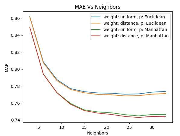
Table of Contents
1. Introduction ..................................................................................................................... 7

 1.1 Related Work ............................................................................................................. 7

 1.2 Research Questions ................................................................................................... 8

 1.3 Aim and Purpose ....................................................................................................... 9

 1.4 Methodology ............................................................................................................. 9

2.Background .................................................................................................................... 10

 2.1 Machine Learning Paradigms .................................................................................. 10

 2.2 Machine Learning Regression Algorithms.............................................................. 11

 2.2.1 Linear Regression ............................................................................................. 11

 2.2.2 K-Nearest Neighbor.......................................................................................... 12

 2.2.3 Decision trees ................................................................................................... 12

 2.2.4 Neural Networks ............................................................................................... 13

 2.2.5 Support Vector Regression ............................................................................... 13

3. Dataset ........................................................................................................................... 14

 3.1 Data Exploration ...................................................................................................... 14

 3.1.1 Movies .............................................................................................................. 14

 3.1.2 Artists ............................................................................................................... 16

 3.2 Data Cleaning .......................................................................................................... 17

 3.2.1 Missing Values ................................................................................................. 17

 3.2.2 Eliminating Redundant Data ............................................................................ 17

 3.3 Data Preparation ...................................................................................................... 18

 3.3.1 Adapting Categorical Columns ........................................................................ 18

 3.3.2 Merging Movies with Artists ........................................................................... 19

 3.4 Final Dataset ............................................................................................................ 20

4. Experiment .................................................................................................................... 21

4.1 Tools Used ............................................................................................................... 21

 4.1.1 Hardware .......................................................................................................... 21

 4.1.2 Software............................................................................................................ 21

 4.2 Algorithm Evaluation .............................................................................................. 21

 4.3 Algorithm Optimization .......................................................................................... 23

 4.4 Limitations............................................................................................................... 24

5. Results ....................................................................................................................... 25

 5.1 Testing and Optimizing Models .............................................................................. 25

 5.1.1 Ridge Regression .............................................................................................. 25

 5.1.2 Lasso Regression .............................................................................................. 26

 5.1.3 K-Nearest Neighbor .................................................................................... 26

 5.1.4 Decision Tree Regression ............................................................................ 27

 5.1.5 Random Forest Regression .......................................................................... 30

 5.1.6 Extreme Gradient Boosting ......................................................................... 31

 5.1.7 Artificial Neural Network ........................................................................... 32

 5.2 Final Results for Multiple Algorithms ................................................................ 35

 5.3 Testing on the New Data .................................................................................... 35

 5.4 Features Importance on Predictions .................................................................... 36

6. Discussion and Analysis ............................................................................................ 37

 6.1 Social and Ethical Aspects ...................................................................................... 39

7. Conclusion ................................................................................................................. 40

 7.1 Future Work ........................................................................................................ 40

8. Bibliography .............................................................................................................. 41

Figures
Figure 1. Visual presentation of a Support Vector Regressor. 13
Figure 2. Movies released from 1900 to March 2021. 16
Figure 3. Genre appearance through movies from 1970 to 2020. 18
Figure 4. Cross validation split with 5 folds. 22
Figure 5. Visual example of overfitting and underfitting. 23
Figure 6. MAE vs alphas in Ridge Regression. 25
Figure 7. Comparing weights and distance formulas with a range of neighbors. 27
Figure 8. MAE vs ‘max_depth’ in a Decision Tree Regression model using MSE 28
 for splitting criteria.
Figure 9. All splitting criteria graphed based on their MAE for predicting movie 29
 ratings with different tree depths.
Figure 10. Poisson splitting criteria on prediction performance for a wide range 29
 of depths.
Figure 11. Random Forest Regression with MSE splitting. Prediction 30
 performance with 100 estimators.
Figure 12. RFR model with a max depth of 27 using MSE for splitting. 31
Figure 13. XGBoost model MAE vs learning rate with early stopping rounds 32
 equal to 5.
Figure 14. MAE vs Neurons with different layers. 34
Figure 15. MAE vs Layers with different neurons. 34
Figure 14. Algorithms Performance on predicting movie ratings with objective 35
 data.
Figure 15. Scatter of predictions vs actual movie rating. 35
Figure 16. Feature Importance of XGBoost excluding the artists. 36
Figure 17. Distribution of movie ratings on trained model. 38

Tables
Table 1. Missing values table. 17
Table 2. Artificial Neural Networks performance based on neurons and hidden 33
 layers.

 5

Terminology
• MAE : Mean Absolute Error
• MSE: Mean Squared Error
• RMSE: Root-Mean Squared Error
• RFR: Random Forest Regression
• XGB: Extreme Gradient Booster
• KNN: K-Nearest Neighbor
• DTR: Decision tree Regression

 6

1. Introduction
Machine Learning is a subfield of Artificial Intelligence, which addresses the question of
how to build computers that improve automatically through experience [1]. In this project,
objective data from movies such as the runtime, directors, actors, region, and genres are
used to train a Machine Learning model. The dataset is provided by the currently biggest
movie dataset in existence, IMDb [2], which is updated daily with more films and TV
shows with further information. IMDb is a website that lets their users inform themselves
about movies and TV shows. As of March 2021, it includes almost 8 million different
titles, growing continuously. Moreover, IMDb also supplies a 10-star rating system based
solemnly on their users’ reviews. The goal of this project is be to predict said rating.

With the power of Machine Learning, present work attempts to find what makes a movie
better for movie watchers using multiple Machine Learning algorithms to find the most
accurate one. Once the best model is found, it can be used to predict the outcome of any
movie, given that the parameters are provided. By the end of the project, two months’
worth of updated data from IMDb is then inputted to the best model to see how well it is
at predicting newer movies. This is the main goal of this thesis. Based on the output, film
studios could make better and more attractive movies for the average audience.

1.1 Related Work
Several similar research projects have already been conducted. This was inevitable with
the current growth of Machine Learning and movie industry’s simultaneous constant
growth.

Kyuhan Lee et al. [3] used naver.com for American movies and IMDb for foreign ones.
Their aim was however to predict the movies’ performances at the box office. This means
that their data is much more budget oriented as well as where the movie was being played
and how many theaters had screenings. They do not explicitly describe the used input
data. In total they achieved a 58.5% accuracy classifying the movies on how much money
the movies profited.

Dorfman, R et al. [4] conducted a research project where they did a similar experiment to
the one to be executed on this project, but the other way around. They took subjective
data to create a model that predicted objectivity. For this purpose, pictures of surgical
patients before and after a rhinoplasty surgery were taken and put into their created age
 7

predicting models to find the effect of the surgery to their apparent age. The result was
that the rhinoplasty did make on average patients look 3 years younger. This research
shows that it is indeed possible to predict objective aspects based on subjective variables.

Xiaodong Ning et al. [5] used a convolutional neural network based on regression for
predicting a movie rating as well. Different from this thesis, they additionaly used Natural
Language Processing to read the plot of the movie. This adds many more variables to
consider and could be inconsistent since they are getting their plots from IMDb which are
done by users, not the actual movie producers.

Yueming Zhang [6] experimented with similar data but also datamined Facebook likes of
the movie, actors and directors. Therefore, they used information that would only be
available after the movie comes out, such as number of votes and gross earnings. The
algorithms used were Decision trees, K-NN and Random Forests, which resulted in a
predictability a bit over 0.7 for all three. 0.7 means that the predictor was in average 0.7
rating points away from the real rating.

Ahmad J et al. [7] used movie information for creating a mathematical model to find
correlations between the genres, actors, and the rating for Bollywood movies. Their
findings showed a strong correlation between both actors and genres for determining the
success of a movie, meaning that some actors perform better on certain genres.

Oghina A et al. [8] extracted likes and dislikes from YouTube videos from what people
said about the movie and textual features from Twitter to train a Linear Regression model
on 10 movies and then tested the model on 60 other movies. The overall focus was on a
comparison between the influence of YouTube likes and dislikes against the Twitter
textual features to measure their influence. The results showed Twitter had a much bigger
influence and mixing them harmed the predictions.

1.2 Research Questions
The present thesis deals in detail with the following research questions:

 • Which algorithm is most applicable for predicting movie ratings and how do they
 compare?
 • How accurately can Supervised Machine Learning techniques predict subjective
 values like a movie’s ratings by using movies’ objective data?

 8

1.3 Aim and Purpose
Movie taste is very complicated as well as always changing at a personal level, however
in a general level, it is more consistent and less variable. This opens the opportunity of
studying that consistency and create predictions with the help of Machine Learning. The
development of this model explores the performance of different Machine Learning
algorithms trained on objective data from movies and with that not only predict ratings
but also see the influence of different features of a movie on the rating and how important
they are as a whole.

1.4 Methodology
This thesis is based on theoretical (literature study) and practical studies.

During the literature study, two main criteria were important: the project’s approach to
movies with some form of Machine Learning or mathematics as well as the disclosure of
the movie features that were used. The Related Work was found by searching on the
databases Google Scholar, Summon, DBLP, and ACM Digital Library. The following
keywords were used: machine learning algorithms, movie rating prediction, IMDb, and
objective data to predict subjective data; with one project coming from Kaggle. Searching
for 10 to 15 papers per keyword with a total of 50 papers, 21 were related enough to be
considered. Only works that were different enough between each other were kept in order
to representing different approaches and ideas.

For the practical study, different Machine Learning Algorithms capable of regression
were tested and validated on the data. Later, the algorithms were optimized and compared.
Finally, the results were discussed to understand their meaning and what they say about
movies’ objective data.

 9

2.Background
Machine Learning focuses on machines teaching themselves with data provided to them,
however there it gets much more complicated as it is learned how that it is prepared and
executed. For building a Machine Learning model, it must first be determined what is
expected from the model or which problem it is trying to solve. Understanding the data
that is used for training the model is essential to know the objective. The five types of
problems generally fall on one of these groups [9]:

1. Classification Problem: When the output needs to be classified into a limited amount
 of groups or sometimes a number.
2. Anomaly Detection Problem: The model monitors some form of phenomena or
 numbers, learning patterns to later detect anomalies.
3. Regression Problem: The output is numeric and continuous, most of the times it is
 represented in trend graphs, their goal is usually avoiding diminishing returns or
 improve profits.
4. Clustering Problem: Similar to a classification problem but it is a form of
 unsupervised learning where it looks for patterns to attempt to build clusters. New
 data goes into the build clusters.
5. Reinforcement Problem: When decisions need to be done based on previous
 experiences, generally learned on an environment. It is reliant on trial and error for
 knowing what are the right decisions to take being “rewarded” for right decisions and
 sometimes “punished” for the wrong ones.

2.1 Machine Learning Paradigms
There are many different types of data or situations that determine which machine
learning paradigms have to be used, usually only one is used but there are situations where
two or more can be used.

1. Supervised Learning: uses concept mapping, feeding the model training data to later
 test it on validation data, everything is labeled.
2. Unsupervised Learning: works with unlabeled data which means there is no test
 data, commonly used with clusters.[10]

 10

3. Semi-supervised Learning: it uses a usually small amount of labeled data for then
 classify all the unlabeled data. A big risk is that errors from the labeled set of data get
 replicated on the unlabeled set [11].
4. Reinforcement Learning: a human-like form of learning by learning through
 interactions with the environment and being rewarded for doing the right thing and
 punished for the wrong thing. Very common for teaching computers to play
 videogames [12].

2.2 Machine Learning Regression Algorithms
Machine Learning relies on algorithms which have complex and advanced mathematics
backing them up with each algorithm being better depending on the desired outcome and
the data that is being fed to it. This project focuses on predicting a movies’ rating, which
is a numeric and continuous variable, therefore the algorithms to be used will be
regression algorithms. Since the data available is already labeled, the model will use
supervised learning to train. The selection process for the algorithms was a combination
of those used by related work and using algorithms that are different enough approaches
to hopefully have found comparable performances between them to compare.

2.2.1 Linear Regression
Linear Regression is a very popular algorithm that works by trying to draw a line through
the training data in a geometrical way and using the line to predict for different inputs.
Commonly, Linear Regression has a whole dimension for each feature of the data. There
are however two other linear algorithms that are more convenient for more complex data
like the two that are used:

Ridge Regression

Ridge regression stabilizes linear regressions by adding a constant to estimate the
coefficients used in the model, also known as a bias. Hence, it is lowering variance and
shrinkage in coefficients which also reduces the model’s complexity [13].

LASSO Regression

LASSO Stands for the Least Absolute Shrinkage and Selection Operator. The goal is to
identify the variables and corresponding regression coefficients to minimize prediction

 11

errors. This is achieved by constraining on the model parameters, “shrinking” the
regressing coefficients to zero [14].

2.2.2 K-Nearest Neighbor
K-Nearest Neighbor is an algorithm that stores all the training data in a n-dimensional
space which means it is memory based. Once an input is sent in, the model looks through
the data to find the nearest k training examples and assigns the label based on those. The
main advantage is it is efficient even with large test data, but its computation cost is very
high [15].

2.2.3 Decision trees
Decision Tree Regressor

This is the most basic form of a decision tree. It builds the model as a large decision tree
formed by a root node with all the data and getting split into smaller nodes until the leaf
nodes are reached, which assigns the value for the output [16].

Random Forest Regressor

For standard trees, the nodes are split by using the best split among all variables while for
a random forest, the best among a subset of predictors, know as gradients, are chosen
randomly to be used for the split. Then in a form of voting, they reach the final prediction.
This might seem to be counter-intuitive since the choosing is random but usually performs
better and is much less heavy to compute[17].

Extreme Gradient Booster

Gradient boosting takes many trees to make an ensemble of them similar to random forest
regressor but then uses the gradient to influence the predictions towards the correct
values. Extreme Gradient Booster (XGBoost) takes it a step further by many hardware
improvements and built for large datasets. It uses the data to extract potential splitting
points based on feature distrbutions and assigns continious values into a bucket of values
to be closer to the feature, greatly reducing the amount of splitting points. Since XGBoost
was made having big datasets in mind, it is aware that most computers’ memory would
not be able to handle it. Therefore, it compresses the data with a separate process to store
it in the disk and decompresses it when loading back into the main memory [18].

 12

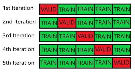
XGBoost is one of the few algorithms capable of using null data as actual data which can
mean more in terms of data than imputed data.

2.2.4 Neural Networks
Neural Networks are based on a brain’s structure using neurons and connections between
them; therefore, they can get very complicated. Neural Networks belong to a whole
subfield of machine learning called deep learning and there are many ways of
approaching them. The structure of a neural network is having several neurons on layers.
In total, there are three types of layers, the input, the hidden and the output layers. The
neurons rely on weights and biases to evaluate the value of each input and propagate
through the hidden layers until the output layer is reached with a hopefully correct
classification [19].

2.2.5 Support Vector Regression
Support Vector Regression works by segregating the training data into different classes
within a space setting a form of boundary called the hyperplane. As a result, any input
will fall into a specific class. The space between the two closest points of different classes
is called the margin. [20]

Figure 1. Visual presentation of a Support Vector Regressor [21].

 13

3. Dataset
The whole dataset must be explored, cleaned, and prepared for a machine learning model
to be able to work on it. This is a crucial part of any form of machine learning as the data
is the only thing that it is provided. Furthermore, it is important to figure out efficient
ways to display data as adding redundant data would make the model more complex and
longer to create while not necessarily providing any more accurate results.

All data is obtained from IMDb directly. The provider updates all their datasets daily and
they are divided into seven different sections which are:

• name.basics.tsv.gz : contains all artists that work on a movie, from actors to editors
 to writers and directors. What their jobs are, the titles they are known for, and age are
 also listed here. Dataset size: (10 million x 6)
• title.akas.tsv.gz : contains information on the title of the movie, its region and
 language. Dataset size: (25 million x 8)
• title.basics.tsv.gz : contains release date, genres, runtime and if the movie is adult
 rated. Dataset size: (7.7 million x 9)
• title.crew.tsv.gz : contains the director(s) and writer(s) of each movie (it is found in
 principals therefore it is not used)
• title.episode.tsv.gz : contains data on which title each episode belongs to (does not
 apply)
• title.principals.tsv.gz : contains the most important people on each movie with their
 role in said movie. Dataset size: (44 million x 5)
• title.ratings.tsv.gz : contains the ratings and number of votes. Dataset size:
 (1.1 million x 3)

3.1 Data Exploration
The data in total can be classified into two fields, movie information and artists
information.

3.1.1 Movies
Starting off with title.basics, it contains all the information of any type of film in IMDb,
that includes TV shows, movies, shorts, etc.. The first thing to do is to drop anything that
is not a movie. Once that is done, for all of the movies data it is needed to merge the new
 14

title.basics, title.akas and title.ratings which combined have a total size of 1.6 million x
18 which is more than title.ratings which has 1.1 million rows, that is because every movie
that gets their title translated is listed while keeping the same titleId. The solution for this
is to remove all duplicates where titleId is the same. Removing the duplicates brings the
dataset to a total of 260,992 movies. However, this counts any movie that was ever done,
no matter how unpopular it might be which means it could alter the predictions.
Fortunately, since IMDb is a website where any user can rate a movie and the title.ratings
dataset provides the number of votes, that can be used to eliminate unpopular movies that
would hinder the Machine learning model. With that in mind, only movies with more
than 1000 votes are considered while the rest are dropped, bringing the data to a total of
32,927 movies.

Additionally, there are a few other things that must be taken into consideration but are
more related to the specific aim of this project rather than to the data itself. IMDb contains
data on all movies, that includes adult rated movies which are not an aim for this project.
Conveniently, the database does provide a column for those movies so they can easily be
removed. This is a very insignificant alteration to the data, reducing the total amount of
movies by 20, which is due to most adult rated films not having a lot of user votes meaning
most of them were already cut out.

Another alteration that must be made to fit this project’s goal is to only count films that
could have the same people working on them to predict future movies. For this to be
achieved, old movies should not be considered. The solution is to remove movies that
were released before the 1970s which is also not a very significant amount since not many
movies were released back then and many of these movies have missing values. This
brings the final count to 28,454 movies.

 15

Figure 2. Movies released from 1900 to March 2021.

This graph shows the number of movies done per year which was constantly increasing
until 2020 when most film releases and production got delayed due to the COVID-19
Pandemic [22]. 2021 also shows low numbers but that is due to the fact that the data was
taken in April 2021.

3.1.2 Artists
Artists have only one dataset with a full list of them and their information such as birth
year and death year if any. With these two fields, it is possible to determine if the artist is
alive which would be relevant for trying to predict upcoming movies. To assure this, a
simple if statement is sufficient, so if deathYear is null, the artist is alive. Some artists do
not have a birthYear and upon inspection, those artists were either very unknown or so
old, there was no data on it. With this in mind, those artists were also removed to avoid
redundant data.

 16

3.2 Data Cleaning

3.2.1 Missing Values
Missing values are a guarantee in Machine Learning when cleaning the data. Therefore,
there are a few approaches that can be used to handle this problem but determining which
approach is best, can sometimes be difficult. The three main approaches are: [23]

• Case deletion: The rows or columns with missing data get deleted under certain
 circumstances.
• Single Imputation: If there is a field with missing data, all data from other rows can
 be used to determine what is most suitable for filling the missing field. This means it
 could be the mean, median or mode. Certain times it is also possible to replace the
 missing value with a 0 but that is more dependent on what the column means than
 other values in the dataset.
• Multiple Imputation: This approach consists of filling the data just as in single
 imputation but also adds a column or a new datasheet where it is marked the missing
 values that were filled. It is generally the best for small datasets.

Starting with the movies, after selecting the relevant values, the missing values within
them were counted and it was found out that 82% of the movies were missing their
language, therefore the language value was immediately dropped, this being a case
deletion approach.

 Values Missing
 Primary Title 0
 Start Year (Release year) 0
 Runtime Minutes 1391
 Genres 36
 Region 14457
 Language 67852
 Average Rating 0
Table 1. Missing values table

3.2.2 Eliminating Redundant Data
With movies’ data having been cut dramatically due to only keeping relatively recent
movies as well as movies with a certain number of votes and genres, any artists that form

 17

part of the movies which were cut that do not participate in movies that are kept, can be
dropped since they would not be important later anyway. This is where the title.principals
dataset is extremely important since it lists the most important artists for each movie,
usually the highest paid 4 actors, the director or directors and sometimes the lead producer
or writer. The approach is to eliminate all the movies from principals that were not in the
new movies data and then continuing with the artists dataset and remove all the artists
that are not in the new title.principals dataset.

3.3 Data Preparation

3.3.1 Adapting Categorical Columns
The region value as it can be seen in Figure 3, has also a quite high missing rate but a
different approach to the language value was taken, One Hot Encoding. One-Hot
Encoding is a way of transforming categorical variables into vectors where all
components are 0 or 1, this in turn would add n-1 columns to the table, where n is the
number of classes to be used and it is minus 1 since the original column is deleted [24].
How it was used here, given that there are over a hundred different regions and adding a
hundred columns to the data would make it unnecessarily big, only the most frequent
regions were assigned to a column and all the remaining regions were sent into a column
named “uncommonRegion” All Regions with over 10 movies were chosen, bringing to a
total of 69 regions plus the uncommonRegion column.

Similarly for genres, a form of One-Hot Encoding was used called Multiple Label
Binarizer. Just like in One-Hot Encoding with the difference being that it is able to split
the values in one same row which is necessary since many movies have more than one
genre. Fortunately, there are not as many total genres as there are regions, so almost all
genres were kept.

 18

Figure 3. Genre appearance through movies from 1970 to 2020.

The removed genres were [Adult, Reality TV, Short and Talk-Show] since they had less
than 10 movies that classified as such.

3.3.2 Merging Movies with Artists
Merging the movies data with the artists could be done in many different ways, some
ideas that were considered were getting the main people that worked on the movie which
is provided by title.principals and then setting their average movie rating as a value in the
training dataset after splitting the validation data and training data to avoid leakage. This
approach was not used since it would be using a non-objective value to predict the result
and would go against the experiment’s purpose.

Another idea was to train a model to predict the rating only using the movie data and use
the artists to predict the deviation from the predicted rating to the real rating, the results
here would be much more directed towards the positive or negative influence artists have
on the previous prediction model so it was also not taken.

Lastly, the approach that was taken was to assign a column to every artist that has
participated in over 10 movies, regardless of role. What made this complicated was that
in title.principals, each important artist of each movie is their own row. Once each artist
has their column, the rows can be grouped if they belong to the same movie and select all
the artists that participate in the movie.

 19

Merging the artists dataset to the movies presented some issues. For example, what if a
movie does not have any of the artists, that would mean the movie is not in principals_data
and all the artists values would be null. In this situation, the single imputation method
was used to fill all the null values with 0. This is logical since if there were no artists with
more than 10 movies, then there would be no column that is not 0.

3.4 Final Dataset
The final artists_movies dataset ended up being an immense table with a very wide width,
having a final size of (28454, 3283), but upon comparing the results of a simple Random
Forest Regression model with and without the artists, there was an improvement. Without
having the artists, the mean absolute error was 0.729, while with it, was 0.684.

The structure of the final dataset consists of the release year of the movie, followed by
the runtime and then 22 different genres, 70 regions and over 3000 artists.

 20

4. Experiment

4.1 Tools Used

4.1.1 Hardware
Device: Gigabyte Aero 15 Laptop

Processor: Intel(R) Core(TM) i7-8750H CPU @ 2.20GHz

RAM: 16.0 GB DDR4-2666

GPU: GeForce GTX 1070 Max-Q

4.1.2 Software
Operating System: Windows 10 64-bit

IDE: IntelliJ IDEA Community Edition

Programming Language: Python

Libraries: Sklearn, Pandas, TensorFlow, XGBoost, Matplotlib

Version Control: Github

4.2 Algorithm Evaluation
In order to compare the algorithms to be implemented there must be a metric to compare
them on. Mean Absolute Error (MAE), Mean Square Error (MSE), and Root-Mean
Squared Error (RMSE) are some of the most common for regression algorithms. Mean
absolute error gets all the delta between the predicted value and the actual value, then
adds them up and then divides it by the number of predicted values, it is a very basic but
efficient way of measuring error. Mean squared error works similarly but squares the
delta, then adds them up and divides them, making it more practical to differentiate
between smaller numbers. RMSE is just the square root of MSE, which is used for
determining accuracy. In this project since a movie can only go from 1.0 star to 10.0
stars, using the MAE makes more sense to get a grasp of how far the average of
predictions are from the real score in average.

 21

The dataset was shuffled with a seed in case there was a need to rebuild it so that it keeps
the same shuffle. The reason for the data being shuffled is the data was in order of how
the movies were added to IMDb, which meant that most old movie were early in the
database and newer ones later in the database. This was found out to be a problem when
the algorithms were tested with cross validation. Cross validation is a form of testing
algorithms where the data is split into parts where one part is used for validating the model
while the other parts are simultaneously used for training the model. The remaining part
is used for validation, using each different part as validation once like so:

Figure 4. Cross validation split with 5 folds.
Before shuffling, the results for a simple Random Forest Regression cross validated in 5
folds were:

[0.9097 0.7151 0.7082 0.6814 0.7181]

Average: 0.7465

And after shuffling the MAE scores for the same Random Forest Regression:

[0.7135 0.7192 0.7235 0.6999 0.6947]

Average: 0.7102

As it can be seen, the results before varied a lot more between which validation set was
used compared to after the shuffle. Therefore, shuffling was done to avoid the need of
cross validating every algorithm to get a more accurate test result since cross validating
with 5 folds logically meant the training and validating of each model would take 5 times

 22

longer. After shuffling, one part of the data was reserved for testing all algorithms and
the rest were used for training.

Algorithms must also be optimized to avoid overfitting and underfitting. Underfitting is
the consequence of not training the model enough to be able to predict accurately,
overfitting is when the model is overtrained and memorizing the training data, performing
poorly when shown new data [25].

Figure 5. Visual example of overfitting and underfitting [25].

4.3 Algorithm Optimization
The algorithms presented in Chapter 2.2 were all tested and evaluated. They all were run
in their simplest and quickest form at first to make sure they were appropriate for the
dataset and computer resources. All of them except Support Vector Regressor were
worked on further for optimizations, the reason being is Support Vector Regressor took
20 hours to completely train and validate a simple model with average results.

All algorithms are to be run on their default configuration and then the model’s
parameters will be tested to find the optimal configuration for lowest MAE. The results
will be graphed in a MAE vs the adjusted parameter thus the graph’s lowest point is the
ideal parameter value. Once all parameters have been optimized, a final model is
considered as that algorithm’s final result. Ultimately, comparing all algorithms, solving
the first research question: “Which algorithm is most applicable for predicting movie
ratings and how do they compare?”

For the second research question: “How accurately can Supervised Machine Learning
techniques predict subjective values like a movie’s ratings by using movies’ objective
data?” The best performing algorithm is then tested on the updated IMDB database,
therefore being tested on movies released since the obtaining of the original dataset
(March 27th, 2021) and the day of final testing (May 13th, 2021).

 23

4.4 Limitations
Support Vector Regressor’s training time was too long for parameter optimizing. Support
Vector Regressors unfortunately do not perform well for large datasets, especially if the
number of features (columns) is large [26].

All models were trained and validated in a computer; no web services were used. Thus,
not having the best processing power and resource availability for the models to be
created. This limits how long some models take to train and limiting the optimization
adjustments that could be made.

 24

5. Results
5.1 Testing and Optimizing Models

5.1.1 Ridge Regression
Ridge Regression only has one parameter that can be adjusted and that is ‘alpha’. α (alpha)
controls the emphasis given to minimizing residual sum of squares vs minimizing sum of
square of coefficients [27]. Basically, it is a measurement as to how fit the model should
be, ideal for avoiding overfitting and underfitting. With the default value, which is either
0.1, 1.0, or 10.0 depending on performance, the MAE result is 0.6658. The MAE for those
three values of alpha were checked:

MAE RR: 0.6928 alpha=0.1

MAE RR: 0.6826 alpha=1.0

MAE RR: 0.6644 alpha=10.0

This means that the value taken was close to 10 but not 10 since alphas=10 performed
better than the default. Hence, alphas of values close to 10 were explored.

Figure 6. MAE vs alphas in Ridge Regression.

 25

Deploying a for loop increasing by 0.1 starting at 9.5 for 12 instances gave the best alphas
value to be 10.1 with an MAE of 0.6643.

5.1.2 Lasso Regression
Lasso Regression is similar to Ridge Regression in that it has a parameter alpha to adjust
the model’s fitting but has the alphas set to 100 as default. Lasso Regression has another
parameter ‘max_iter’ that can control the maximum number of iterations which by default
is 1000. The final parameter that can be changed is ‘normalize’ which is a simple Boolean
that is false by default. Normalizing means the regressors X will be normalized before
regression by subtracting the mean and dividing by the l2-norm [28].

The default Lasso model gave a MAE of 0.7307 and the same model with the parameter
‘normalize’ set to true gave a MAE of 0.6674. Adjusting any of the other two parameters
did not change the MAE, consequently no further adjustments were done.

5.1.3 K-Nearest Neighbor
K-Nearest Neighbor has many parameters. For level of optimizing in this project, only
three are adjusted. All the variables are defined and set by Sklearn [29]

 • ‘n_neighbors’: number of neighbors that will be considered to predict. By default,
 it is 5.
 • ‘weight’: it means how much influence the neighbors have on the value to predict.
 there are two usual options {‘uniform’, ‘distance’} and a third one that is user-
 defined, which is not tested. The default is ‘uniform’, and it means that all
 neighbors carry the same weight. Measuring weight through their distance means
 that the closer the neighbor is, the larger the influence it has.
 • ‘p’: stands for power parameter and it determines the distance equation to use. 1
 for Manhattan Distance and 2 for Euclidean Distance. Default is Euclidean.

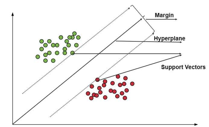
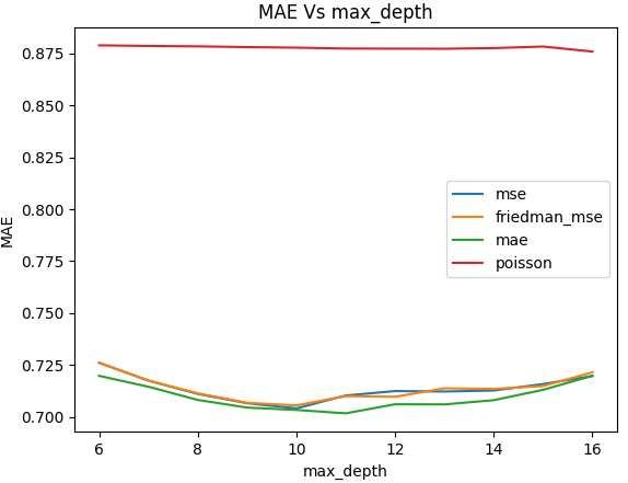
 26

Figure 7. Comparing weights and distance formulas with a range of neighbors.

With the results listed above, Manhattan Distance formula was better than Euclidean as
well as measuring the weight is slightly worse if measured uniformly. It must be pointed
out that using Manhattan Distance however, took over 5 hours for both weights while
Euclidean took 10 minutes. This is probably because Manhattan requires performing
multiple sums of lines that each traverses one dimension to reach the goal while Euclidean
is just one line through multiple dimensions. No noticeable time difference was found
between weighing the influence of neighbors by distance other than uniformly. The best
MAE was 0.7449 with 27 neighbors, weight: distance and using Manhattan Distance
formula to measure distance.

5.1.4 Decision Tree Regression
Decision Tree Regression can use multiple criteria for when splitting the tree is best, the
criteria provided by Sklearn [30] are MAE, MSE (default), Friedman_MSE and Poisson.
Friedman_MSE is like MSE but implements the Friedman test, it works by first ranking
the data and testing if different columns could come from the same “universe” [31].
Finally, Poisson that uses Poisson deviance, uses the following formula:
 27

 
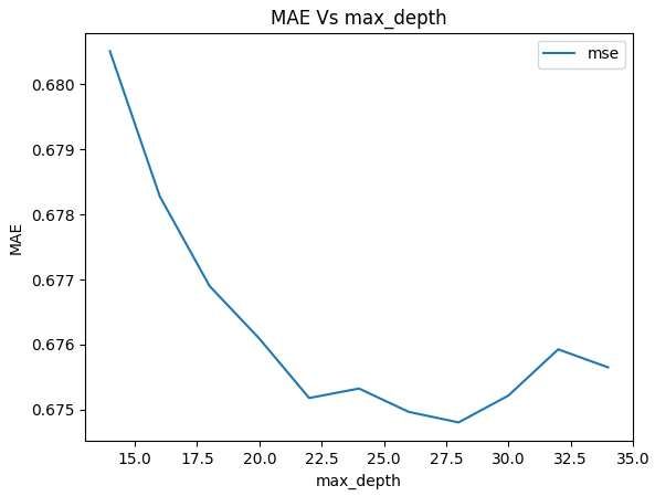
 = 2 ∑[ log (̂ ) − ( − ̂ )] (Eq 1)
 
Where D is the deviance, ̂ are the predictions and is the ground truth [32].

The other very important parameter for a Decision Tree Regression model is the
maximum depth of the tree. Without setting a limit to it and using MSE as splitting
criteria, the depth is 160 levels and 20824 leaf nodes and an MAE of 0.8802. The depth
of a tree is very important to avoid overfitting, therefore the maximum depth must be
adjusted. Testing the ‘max_depth’ in the MSE model, it was found out that 160 was
severely overfitted.

Figure 8. MAE vs ‘max_depth’ in a Decision Tree Regression model using MSE for splitting criteria.

The best fit for a DTR model using MSE was having a ‘max_depth’ of 10, resulting in a
prediction MAE of 0.7041, significantly better than not setting a ‘max_depth’. The other
splitting methods are therefore going to be tested with similar ‘max_depth’s

 28

Figure 9. All splitting criteria graphed based on their MAE for predicting movie ratings with different tree
depths.
Ironically, the MAE splitting criteria was the best at depth 11 with a prediction MAE of
0.7017 having 572 node leaves. But just like the K-Nearest Neighbor, the best performing
model takes significantly longer to train than other ones for a small improvement. The
Poisson splitting criteria behaved very differently from the other 3, having the best results
at a depth of 92 with a MAE of 0.8425 which is still significantly worse than the other
splitting methods.

Figure 10. Poisson splitting criteria on prediction performance for a wide range of depths.

 29

5.1.5 Random Forest Regression
Random Forest Regression has 3 main parameters to adjust:

 • Max depth: Same principle as DTR.
 • N-Estimators: Controls the amount of trees in the forest.
 • Criterion: Exactly like DTR but only has the options of MSE and MAE. Using
 MAE however, takes around 4 hours per trained model, making it hard to
 optimize. For that reason, MAE will not be tested.

A default RFR model would consist of 100 estimators using MSE as splitting criteria and
no depth limit with a result of 0.7246.

Deciding the max depth should be done first since it is dependent on the data while the
number of estimators is dependent on the data and depth.

Figure 11. Random Forest Regression with MSE splitting. Prediction performance with 100 estimators.

Now that the best depth is known to be 27 with an MAE of 0.6746, the number of
estimators can be adjusted.

 30

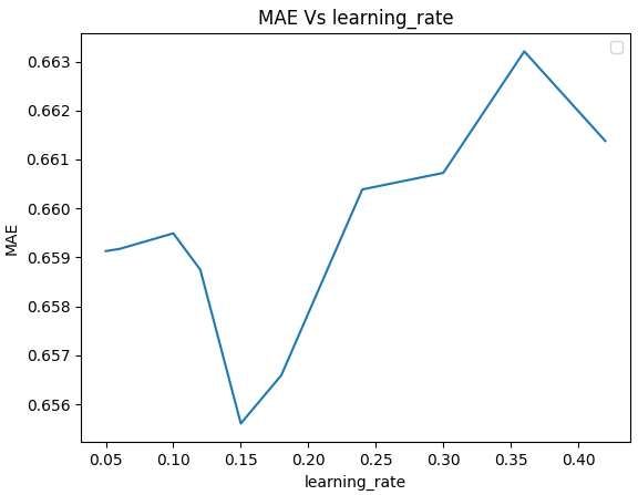
Figure 12. RFR model with a max depth of 27 using MSE for splitting.

Finally, RFR reached an MAE of 0.6744 with 75 estimators and a max tree depth of 27.
It must be pointed out the miniscule impact that the number of estimators had, from the
worst performing with 25 estimators only being 0.3% better.

5.1.6 Extreme Gradient Boosting
XGBoost is one of the most powerful algorithms for regression and that is due to its
complexity and efficiency but also the available parameters [33]. One of the most
valuable ones is the ‘early_stopping_rounds’. What it does is for the model to
automatically stop training when the validation score stops improving, finding the ideal
number of estimators. It is set as an integer and that integer represents how many
iterations of the model not improving the model must go through to stop. This completely
removes the need to adjust the estimators and thus avoids overfitting in that regard.

Another important parameter is ‘learning_rate’ which also combats overfitting by
multiplying the predictions of each model by the value it is set to be. Consequently, each
tree that is added to the ensemble helps less, allowing for a higher number of estimators
without overfitting.

 31

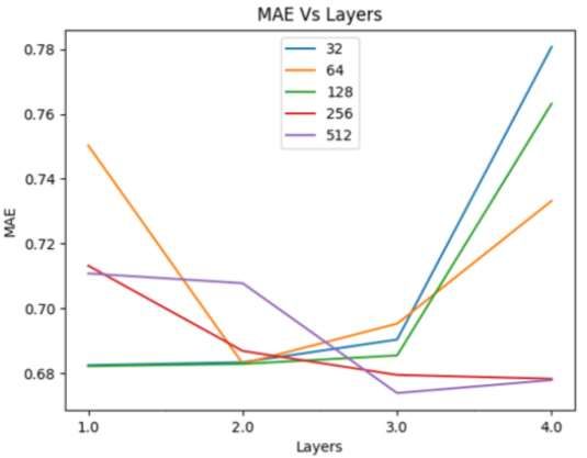
A default XGBoost model is already better than most other algorithms with a result of
0.6623, this is without early stopping rounds or learning rate and faster than any other
algorithm. After setting up a model with early stopping rounds of 5 and a changing
learning rate, this are the results:

Figure 13. XGBoost model MAE vs learning rate with early stopping rounds equal to 5.

The XGBoost model has performed best out of all other algorithms with the best model
having a MAE of 0.6556 at a learning rate of 0.15 while still being a quick algorithm to
train and validate with.

5.1.7 Artificial Neural Network
There are a lot of approaches that can be taken to not only improving but building an
Artificial Neural Network, that is the reason there is a whole field dedicated to it. The
neural networks are built as sequential models from Keras [34].

Neural Networks basic structure is open for a lot of options, for the extent of this project,
four neural networks are created. In order to find the best amount of hidden layers and
neuros, some form of trial and error will be done. There will be sixteen combinations of
networks, having 1 through 4 hidden layers and 32, 64, 128, 256 or 512 neurons. All
 32

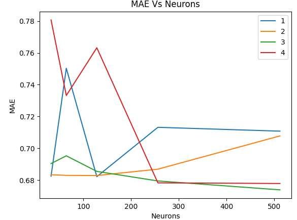
twenty neural networks have a max number of epochs of 100 and a patience of 5. Epochs
are iterations through the data, similar to estimators; patience is exactly like early stopping
rounds but for epochs instead of estimators. Each layer (except the output layer) uses
ReLU (Rectified Linear Unit) for its activation function.

Activation functions are responsible for determining which neurons get activated and
which do not. The reason for using ReLU is that it is considered “one of the few
milestones in the deep learning revolution” [35]. ReLU however it is very simple, if the
input is zero or negative, it returns zero, otherwise it returns the input. It is thanks to its
simplicity that it is so efficient and fast to use for training.

The networks are then compiled with the ‘Adam’ optimizer which is one of the most
efficient optimizers and requires a low amount of memory. Its name comes from adaptive
moment estimation, and it gets that name because it uses different learning rates for
different parameters established by estimates done by the gradients [36]

Finally, the loss function to be used is MSE, the other option is MAE, but both were tested
on a 64 neuron and 2 hidden layers model, the neural network with a loss function of
MAE had and MAE in predictions of 0.6826 while MSE had a MAE 0.683 yet the MSE
took three times as long to execute while no big improvement was noticed and when
performed in the dataset without the actors performed slightly worse when compared on
the second layer.

 Neurons\Hidden 1 2 3 4
 Layers
 32 0.6825 0.6834 0.6904 0.7807
 (32 epochs) (41 epochs) (38 epochs) (24 epochs)
 64 0.7503 0.683 0.6953 0.7332
 (24 epochs) (57 epochs) (51 epochs) (24 epochs)
 128 0.6822 0.6829 0.6855 0.7632
 (58 epochs) (26 epochs) (46 epochs) (45 epochs)
 256 0.7132 0.6869 0.6795 0.6783
 (39 epochs) (32 epochs) (30 epochs) (31 epochs)
 512 0.7108 0.7078 0.6739 0.6779
 (7 epochs) (42 epochs) (79 epochs) (38 epochs)
Table 2. Artificial Neural Networks performance based on neurons and hidden layers.

 33

Figure 14. MAE vs Neurons with different layers.

Figure 15. MAE vs Layers with different neurons.

 34

5.2 Final Results for Multiple Algorithms
The following chart shows the best performing models of each algorithm. The y axis of
the chart represents and increasing MAE, therefore the lower the bar, the better the model:

 Algorithms Performance
 0.76
 0.74
 0.72
 0.7
 0.68
 0.66
 0.64
 0.62
 0.6
 Ridge Lasso KNN DTR RFR XGB ANN

Figure 16. Algorithms Performance on predicting movie ratings with objective data.

5.3 Testing on the New Data
Now that the best algorithm for predicting movie ratings is known, it can be tested on
newer data. The new data from IMDB from May 13th, 2021 was obtained and the
algorithm as tested on it. The MAE for this test was 0.7384.

Figure 17. Scatter of predictions vs actual movie rating.
 35

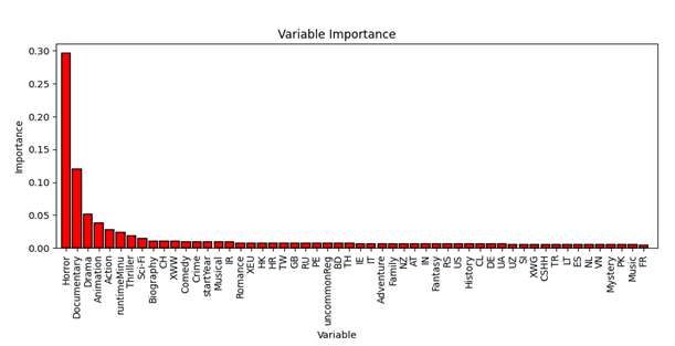
With this same test on new data, it is possible to obtain the R-squared of the model. R-
squared is a form of measurement in statistics that calculates the influence the features
measured over the rating [37]. In other words, what percentage of a movie’s ratings
depends on the data used for the model, in this case a movie’s objective data. In order to
calculate the R-Squared the following formula is used:

 ∑ 
 =1( − )
 2
 2 = 1 − ∑ 2
 (Eq 2)
 =1( − )

 ℎ ℎ 

The result gives an R-squared of 0.311 or 31% therefore the features used in the model
make up for around a third of a movies’ rating.

5.4 Features Importance on Predictions
To check the importance of each feature for the prediction, the best performing algorithm,
XGBoost was taken and used on a dataset without the artists. This model although trained
on a dataset without the artists, still performed quite well with a MAE of 0.6902 and the
importance values are similar to the original while scaled up to ignore the artists. The
features shown make up 90% of all influence and 57% of all features:

Figure 18. Feature Importance of XGBoost excluding the artists.

 36

6. Discussion and Analysis
The algorithms executed in the project all got similar results with some variations. The
standout of the results being Extreme Gradient Boosting, with the best predicting model
and one of the fastest to train. Two other important algorithms to mention are Ridge and
Lasso Regression, getting good performances in relation to others, while being the
simplest algorithms tested. All models however, arrived at similar results consequently
there is not much optimization that could be done.

Some models used algorithms that took significantly more time than their counterparts
while providing little to no improvement, in scenarios where the prediction is of extreme
importance, it would be worth attempting to improve the best model even further. At a
certain point, the optimization reaches a point of diminishing returns where the resources
to be put into improvement of a model start becoming more important. In the case of
regression algorithms of the feature (column) size of this project, improvement becomes
very expensive quickly.

The Neural Network results are a perfect representation of why Deep Learning is a
complicated field, there is no immediately apparent explanation as to how those results
came to be. The results show an improvement in the row for 256 neurons when layers
were added and in the column for 3 hidden layers, almost all other rows show a worse
performance as layers were added. There was no apparent pattern for the change in
performance as the neurons changed when the layers stayed the same.

Some variables that could have been very useful for the prediction had many missing
values for a lot of movies like language. IMDb also does not provide a movie’s budget or
PG rating in their database which was used on other similar studies that used data mining
or different ways of obtaining the data. The number of artists that were included in the
dataset that was used for training the model was limited and using more could have been
beneficial.

The dataset includes movies form 1970 until May 2021 but IMDB was released in 1990
and did not have much popularity until a bit before Amazon purchased it in 1998 [38].
That means that any movies from 1970 to 1990 were always rated as a movie that was
already old, compared to new released which can be influenced more by people having
just gone to the movies. The demographics of the people which the movies were oriented

 37

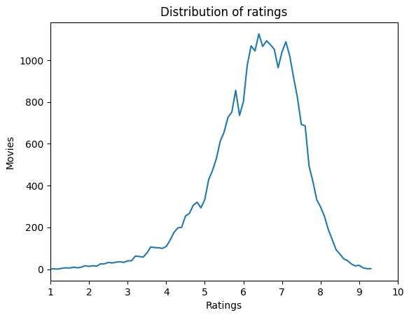
to could also have a great impact on the movie rating which cannot be filtered. This is
related to the fact that the rating distributed by IMDb just shows the rating without
showing the dispersion of the votes, which could be very valuable for predicting as well.

Using the newer IMDB data, getting a result of 0.7384 as the MAE is to be expected due
to the previous statements, the data the model was trained on is from old and new movies
while the newer data is mainly composed of newer movies. There are some old movies
as well since the data was extracted in the same fashion and some movies from the past
could have reached over 1000 votes and therefore make the cut. With the scatter graph it
becomes clear that the model is not as accurate as the number 0.7384 might seem since
the majority of movies are between 5 and 8 stars therefore it is hard to get a bigger error.
Checking the data with which the model was trained, most votes are between 5 and 8 as
well. In fact, 85% of the ratings are between 5.0 and 8.0.

Figure 19. Distribution of movie ratings on trained model.
The R-squared obtained further signals at how big a MAE of 0.7 is. If 31% of a movies’
rating is determined by the objective data used, then that means that the other 69% is
marketing, word of mouth, and of course everything that literally makes a movie like
dialogue, directing, story, edition, acting, etc.

 38

The importance of the variables is very disperse. The importance does not mean however
there is a positive or negative influence, it just measures influence. For example, the
feature horror being so much more important than others means that horror movies follow
a much more apparent pattern than any other feature. This means that knowing if a movie
is horror or not has a big impact on the predicted rating for this model.

6.1 Social and Ethical Aspects
The purpose for this thesis was to prove which algorithm was better which was found out,
but technology is constantly changing therefore the results of this project are bound to
become outdated. However, this thesis contributes to the idea of humans being somewhat
predictable creatures, at least in the masses. This is a consequence of the Data Revolution
[39] where all data is stored and can be processed to find patterns and then used for some
form of benefit. In this case it could be used for filmmakers to compare the cost of an
actor performing in certain movie to the actual value it provides to the movie and decide
if it is a good deal or not. Furthermore, it can be used the other way around for actors that
feel underpaid, this information could provide proof as to what they are providing to the
movies they participate on in an objective form.

 39