Water for food: The global virtual water trade network
←
→
Page content transcription
If your browser does not render page correctly, please read the page content below
WATER RESOURCES RESEARCH, VOL. 47, W05520, doi:10.1029/2010WR010307, 2011

Water for food: The global virtual water trade network
M. Konar,1 C. Dalin,1 S. Suweis,1,2 N. Hanasaki,3 A. Rinaldo,2,4 and I. Rodriguez‐Iturbe1
Received 6 December 2010; revised 15 February 2011; accepted 24 February 2011; published 17 May 2011.

[1] We present a novel conceptual framework and methodology for studying virtual
water trade. We utilize complex network theory to analyze the structure of the global
virtual water trade associated with the international food trade. In the global virtual water
trade network, the nations that participate in the international food trade correspond
to the nodes, and the links represent the flows of virtual water associated with the trade
of food from the country of export to the country of import. We find that the number
of trade connections follows an exponential distribution, except for the case of import trade
relationships, while the volume of water that each nation trades compares well with a
stretched exponential distribution, indicating high heterogeneity of flows between nations.
There is a power law relationship between the volume of virtual water traded and the
number of trade connections of each nation. Highly connected nations are preferentially
linked to poorly connected nations and exhibit low levels of clustering. However, when
the volume of virtual water traded is taken into account, this structure breaks down.
This indicates a global hierarchy, in which nations that trade large volumes of water are
more likely to link to and cluster with other nations that trade large volumes of water,
particularly when the direction of trade is considered. Nations that play a critical role
in maintaining the global network architecture are highlighted. Our analysis provides the
necessary framework for the development of a model of global virtual water trade aimed
at applications ranging from network optimization to climate change impact evaluations.
Citation: Konar, M., C. Dalin, S. Suweis, N. Hanasaki, A. Rinaldo, and I. Rodriguez‐Iturbe (2011), Water for food: The global
virtual water trade network, Water Resour. Res., 47, W05520, doi:10.1029/2010WR010307.

1. Introduction                                                           [3] International trade links the fortunes and resources
                                                                       of countries, providing potentially important conduits for
   [2] Global freshwater resources are finite and subject
                                                                       geographically limited water resources to be transferred to
to increasing pressures from population growth, economic
                                                                       water‐stressed regions. The virtual water trade between
development, and climate change [Vorosmarty et al., 2000;              regions [Hoekstra and Hung, 2005; Chapagain et al., 2006;
Gleick, 2008; Strzepek and Boehlert, 2010]. The vast
                                                                       Yang et al., 2006; Hanasaki et al., 2010] and the gross
majority (90%) of global freshwater use is for food produc-
                                                                       virtual water flow of nations [Chapagain and Hoekstra,
tion [Shiklomanov, 1997; Oki and Kanae, 2004; Hoekstra
                                                                       2008] have been quantified. These studies have focused
and Chapagain, 2008], which is why much attention and
                                                                       primarily on agricultural commodities [Hoekstra and Hung,
research has been devoted to the use of water in agriculture.
                                                                       2005; Liu et al., 2007; Rost et al., 2008; Hanasaki et al.,
In fact, there is a growing body of literature that focuses
                                                                       2010], including those used for biofuel production [Gerbens‐
on the water that is embodied in the production and trade of
                                                                       Leenes et al., 2009], but the concept has also been extended
agricultural commodities, referred to as “virtual water.” Since
                                                                       to include industrial products [Chapagain and Hoekstra,
the concept was first introduced by Allan [1993], there has
                                                                       2008]. However, the global properties of virtual water trade
been a dramatic increase in the virtual water literature, largely      have not yet been quantified or explored. In this paper we build
in an attempt to quantify its potential to alleviate regional
                                                                       upon the virtual water literature and utilize complex network
water scarcity and save water globally [Chapagain et al.,
                                                                       methods to characterize the global structure of the virtual water
2006; Yang et al., 2006; D’Odorico et al., 2010].
                                                                       trade associated with the international food trade.
                                                                          [4] The origin of complex network theory can be traced
                                                                       back to the work of Erdös and Rényi [1961] on random
  1                                                                    graphs. Recently, much research has been devoted to the
    Department of Civil and Environmental Engineering, Princeton
University, Princeton, New Jersey, USA.                                field of complex network analysis, both theoretically and as
  2
    Laboratory of Ecohydrology, ECHO/IEE/ENAC, École Polytechnique     applied to real‐world systems [Barabási and Albert, 1997;
Fédérale de Lausanne, Lausanne, Switzerland.
  3
                                                                       Newman et al., 2006]. This recent interest in complex net-
    National Institute for Environmental Studies, Tsukuba, Japan.      works is largely due to the discovery of organizing princi-
  4
    Department IMAGE and International Centre for Hydrology
“Dino Tonini,” Università di Padova, Padua, Italy.                     ples in networks [Costa et al., 2007], such as community
                                                                       structure [Watts and Strogatz, 1998] and scale‐free proper-
Copyright 2011 by the American Geophysical Union.                      ties [Barabási and Albert, 1997]. Additionally, network
0043‐1397/11/2010WR010307                                              analysis has become increasingly popular because of its

                                                                W05520                                                          1 of 17
W05520 KONAR ET AL.: NETWORK ANALYSIS OF GLOBAL VIRTUAL WATER W05520
flexibility and generality for representing many natural properties of virtual water trade jointly with individual roles
structures [Barabási, 2002; Costa et al., 2007], including and mutual interactions of single nations within the overall
street systems [Kalapala et al., 2006; Masucci et al., 2009], the network architecture. Not only is this type of analysis
internet and World Wide Web [Barabási and Albert, 1997], fascinating in its own right, but it is our hope that future
international tourism [Miguens and Mendes, 2008], financial extensions of this work will illuminate unprecedented
transactions [Garlaschelli and Loffredo, 2005; Kyriakopoulos opportunities to save water globally and serve as a tool for
et al., 2009], Hollywood actors, and scientific collaborations impact assessment, particularly under future scenarios of
[Newman, 2001; Barrat et al., 2004], among others. climate change, whose impacts on the linked water and food
[5] We present a novel application of network theory to systems will likely be captured by changes in global virtual
the global virtual water trade. The global virtual water trade water flows. In particular, in order to develop a theoretical
forms a weighted and directed network in its complete network model [Suweis et al., 2011] that may account for
representation. A weighted network is one in which values the structural features of real‐world virtual water trade,
are associated with the links of the network, while a directed we must first be able to frame what those features are [e.g.,
network is one where the links connect nodes in a particular Newman et al., 2006]. Hence, a thorough analysis of
direction [Wasserman and Faust, 1994; Newman, 2003; empirical data of the type presented in this paper is essential.
Newman et al., 2006; Jackson, 2008]. For the virtual water
trade network, the links are assigned a weight on the basis of 2. Building the Global Virtual Water
the volume of virtual water that is traded between countries Trade Network
and a direction according to the direction of the underly-
ing commodity trade flow (i.e., from exporter nation to [8] Here we describe the construction of the global virtual
importing nation). In this paper, we study the virtual water water trade network. In the network, each country partici-
trade network associated with the trade of 58 agricultural pating in food trade is represented by a node. Links between
commodities from five major crops (i.e., barley, corn, rice, nodes are directed on the basis of the direction of trade flow
soy, and wheat) and three major livestock products (i.e., and are weighted by the volume of virtual water embodied
beef, pork, and poultry) in the year 2000. These products in the traded commodities. To construct this network, we
account for approximately 60% of global calorie consump- require two main pieces of information: the crop trade
tion (Food and Agriculture Organization of the United between all nations and the virtual water content of each
Nations (FAO), FAOSTAT, 2010, http://faostat.fao.org/site/ crop in all nations. For a complete list of the commodities
291/default.aspx, hereinafter referred to as FAOSTAT, considered in this paper refer to Table 1. We obtain the
2010). There are 166 nations that participate in the export of bilateral trade of agricultural products from the FAO. To
these commodities and 151 that import these commodities, calculate the virtual water content of the commodities, we
comprising the nodes of the network. The volume of virtual utilize the H08 global hydrological model [Hanasaki et al.,
water that is traded globally is 625 × 109 m3 yr−1, which 2008a, 2008b]. Virtual water flows between nations are then
accounts for approximately 10% of the global freshwater calculated by multiplying the international trade flow of a
use in agriculture, or 8% of total global water use [Hoekstra particular commodity by the associated virtual water content
and Chapagain, 2008]. of that commodity in the country of export.
[6] Complex network theory has been used to character- 2.1. Virtual Water Content Data
ize the world trade web weighted by the financial value of
[9] We calculated the virtual water content of five
traded commodities (e.g., refer to Garlaschelli and Loffredo
unprocessed crops (barley, corn, rice, soy, and wheat) and
[2005], Fagiolo et al. [2008], Kyriakopoulos et al. [2009],
and Barigozzi et al. [2010]). In this paper, we analyze the three livestock products (beef, chicken, and pork) for each
nation by water withdrawal source using the H08 global
network structure of global virtual water trade associated
hydrological model [Hanasaki et al., 2008a, 2008b]. Virtual
with the international food trade. Thus, we apply the tools of
water content (VWC, kg water kg−1 product) of raw crops is
complex network theory to a subset of the world trade web.
defined as the evapotranspiration during a cropping period
However, the major departure between our analysis and
(kg m−2) divided by the crop yield (kg m−2). The VWC of
other network studies of world trade centers on the weights
unprocessed livestock products is defined as the water
(i.e., value) assigned to the trade flows. We assign weights
consumption per head of livestock (kg head−1) divided by
to links in the international food trade on the basis of the
the livestock production per head (kg head−1). A brief
volumes of water embodied in a given trade relationship,
description of the H08 model is provided here; for further
while other studies of the world trade web in the literature
assign weights in terms of financial values [Garlaschelli information the interested reader is referred to Hanasaki
et al. [2010].
and Loffredo, 2005; Fagiolo et al., 2008; Kyriakopoulos
[10] The H08 model consists of six modules: land surface
et al., 2009; Barigozzi et al., 2010]. Additionally, we ana-
lyze both the directed and weighted properties of the net- hydrology, river routing, crop growth, reservoir operation,
environmental flow requirements estimate, and anthropo-
work, which is seldom done in the literature, with rare
genic water withdrawal. The model operates on a 0.5° × 0.5°
exceptions like the work of Miguens and Mendes [2008].
grid spatial resolution with water and energy balance clo-
[7] Scientific understanding of natural hydrological pro-
sure. Two types of input data are necessary to run the H08
cesses has dramatically increased over the past 50 years [Oki
model: meteorological forcing and land use. Using the H08
and Kanae, 2004]. Now a similar quantitative representation
model, we are able to assess the two major sources of vir-
of the social aspects of water use is necessary. With this goal
tual water content: precipitation (“green water”) and irriga-
in mind, we analyze the global structure of virtual water
tion (“blue water”) [Falkenmark and Rockstrom, 2004].
trade. The network analysis presented here highlights global
2 of 17W05520 KONAR ET AL.: NETWORK ANALYSIS OF GLOBAL VIRTUAL WATER W05520
Table 1. List of Commodities and the Yield Ratio r, Price Ratio p, [11] The virtual water content of unprocessed crop com-
and Content Ratio ca modities (dimensionless) is calculated as
Ratio
ETe;c;s
r p c VWCe;c;s ¼ ; ð1Þ
Ye;c
Crop Commodities
Wheat 1 1 1
Flour of wheat 0.78 0.97 1 where ET is the evapotranspiration during a cropping period
Bran of wheat 0.22 0.024 1 (kg water m−2) and Y is the crop yield (kg crop m−2). The
Macaroni 0.78 0.97 1 subscripts e, c, and s denote the exporting country, crop, and
Germ of wheat 0.025 0.01 1
Bread 0.78 0.97 0.71 water withdrawal source, respectively. To transform the
Bulgur 1 1 1 VWC of raw crops into that of a processed commodity,
Rice, paddy 1 1 1 (1) is multiplied by pxcx/rx. The price ratio (p) is the ratio
Rice, husked 0.72 1 1 between the price of the raw crop and the commodity pro-
Milled husked rice 0.72 1 1 duced from that raw crop. The content ratio (c) indicates
Rice, milled 0.65 0.95 1
Rice, broken 0.65 0.95 1 the fraction of crop origin ingredients in unit commodities.
Bran of rice 0.07 0.049 1 The yield ratio (r) quantifies the fraction of ingredients in
Rice, bran oil 0.013 0.049 1 raw crops. Values of r, p, and c are specific to commodity
Cake rice bran 0.057 0.049 1 x (r, p, and c for each of the 58 commodities are provided in
Rice, flour 0.65 0.95 1
Rice, fermented beverages 0.48 0.95 0.36 Table 1, originally provided by Hanasaki et al. [2010]).
Barley 1 1 1 Although crop yield was an output of the H08 model, data
Pot barley 0.46 0.76 1 from the FAO (FAOSTAT, 2010) was used for increased
Barley, pearled 0.46 0.76 1 reliability in the calculation of VWC.
Bran of barley 0.54 0.24 1
Barley flour and grits 0.46 1 1
[12] The VWC of unprocessed livestock products (dimen-
Malt 0.78 1 1 sionless) is calculated as
Malt extract 0.78 1 0.8
Beer of barley 0.78 1 0.14 WCe;l;s
Maize 1 1 1 VWCe;l;s ¼ ; ð2Þ
Germ of maize 0.115 0.18 1 Pe;l
Flour of maize 0.8 0.75 1
Bran of maize 0.085 0.068 1 where WC is the water consumption per head of livestock
Maize oil
Cake of maize
0.04
0.075
0.18
0.18
1
1
(kg water head−1) and P is the livestock production per head
Soybeans 1 1 1 (kg livestock head−1). The subscripts e, l, and s denote the
Soybean oil 0.19 0.35 1 exporting country, livestock product, and water withdrawal
Cake of soybeans 0.76 0.65 1 source, respectively. To transform the VWC of unprocessed
Soya sauce 0.76 0.65 0.17 livestock products into that of a processed commodity, (2) is
Maize, green 1 1 1
Maize for forage and silage 1 1 1 multiplied by pxcx/rx. The coefficients p, c, and r have the
same meaning as they do for the crop coefficients, and their
Livestock Products values for livestock commodities can be found in Table 1.
Cattle meat 0.6 0.61 1 WC was calculated by estimating the virtual water content
Offal of cattle, edible 0.32 0.38 1
Fat of cattle 0.04 0.0024 1
of livestock feed. Next, the required livestock feed per head
Meat cattle boneless 0.6 0.61 1 was estimated taking into account the life cycle of livestock.
(beef and veal) Then water use other than feed, such as drinking and
Cattle, butchered fat 0.04 0.0024 1 cleaning water, was added.
Preparation of beef 0.4 0.61 1 [13] Graphs of the mean VWC are shown in Figure 1. The
Pig meat 0.7 0.88 1
Offal of pigs, edible 0.12 0.12 1 mean VWC for each of the six world regions (United Nations,
Fat of pigs 0.06 0.006 1 Composition of macro geographical (continental) regions,
Pork 0.49 0.88 1 2010, http://unstats.un.org/unsd/methods/m49/m49regin.htm,
Bacon and ham 0.49 0.88 1 hereinafter referred to as United Nations, 2010) is illustrated
Pig, butchered fat 0.06 0.006 1
Pork sausages 0.49 0.88 1
in Figure 1a, separated into livestock and crop categories. The
Prepared pig meat 0.49 0.88 1 globally averaged VWC for each of the unprocessed livestock
Lard 0.06 0.006 1 and crop products is provided in Figure 1b.
Chicken meat 0.53 0.95 1
Offal and liver of chicken 0.022 0.014 1 2.2. Food Trade Data
Fat liver prepared (foie gras) 0.022 0.014 1
Chicken meat canned 0.53 0.95 1 [14] International food trade statistics list 58 commodities
Fat of poultry 0.022 0.013 1 (shown in Table 1) that contain barley, corn, rice, soy,
Fat of poultry, rendered 0.022 0.013 1 wheat, beef, chicken, or pork. The annual trade matrix (T)
a
Modified from Hanasaki et al. [2010]. of these 58 commodities was obtained from the FAO
(FAOSTAT, 2010) for 233 nations in the year 2000. For any
discrepancy in the trade volume reported between two
Blue water evapotranspiration was further subdivided into nations, the average was taken, with the exception of cases
three categories on the basis of the water source: stream- in which no trade was reported by one of the nations, for
flow, medium‐size reservoir, and nonrenewable and non- which we use the reported trade values. When no data were
local water.
3 of 17W05520 KONAR ET AL.: NETWORK ANALYSIS OF GLOBAL VIRTUAL WATER W05520
Figure 1. Mean virtual water content (VWC) by water source. The blue portion of the bar represents the
blue VWC; the green portion shows the green VWC. (a) Mean VWC for each of the six regions: Africa
(Af), North America (NA), South America (SA), Asia (As), Europe (E), and Oceania (O). The thick bars
represent the mean VWC for the livestock products: beef, pork, and poultry. The thin bars show the mean
VWC for the crops: barley, corn, rice, soy, and wheat. (b) Global average VWC for each of the unpro-
cessed livestock and crop products: beef (Bf), chicken (Ck), pork (P), soy (S), barley (Br), corn (Cr),
wheat (W), and rice (R).
reported between two nations, we assumed that no trade exists between two nodes that trade with one another. Each
occurred between those two nations. link is directed on the basis of the trade flow direction and is
weighted by the volume of virtual water. A network map is
2.3. Network Construction provided in Figure 2. For any pair of nodes (i, j) the matrix
[15] The VWC and T data in combination allow us to element WD(i, j) represents the volume of water traded from
construct the global virtual water trade network (W). In this node i to node j (i.e., node i exports to node j). Note that WD
network, each nation is expressed as a node, and the links is not symmetric and W(i, i) = 0; that is, a country cannot
represent the volume of virtual water flow between nations. trade with itself. In the FAO trade data there was one
We calculate the virtual water flows between nations by instance, the case of Venezuela, of a country reporting trade
multiplying the crop and livestock trade between nations by with itself. We determined that this data point was erroneous
the VWC of that crop or livestock product in the country of and set it equal to zero.
export. The network connections are thus determined by the [18] From the complete network with information on link
agricultural trade relationships and the weight of each con- weights and direction, we create simpler networks: the
nection by the volume of virtual water embodied in the crop weighted, undirected network (WU); the unweighted, directed
and livestock trade. network (AD); and the unweighted, undirected network (AU).
[16] The total virtual water trade is thus expressed as An unweighted network is referred to as an adjacency matrix
" # (A). We create these simpler networks to assess network
X X px cx topology with and without link weights and direction. First,
We;i ¼ VWCe;a;s Te;i;x ; ð3Þ WU was created by symmetrizing the directed, weighted
s;c x2a
rx
network on the basis of the sum of the link weights between
two nodes. This symmetrization creates an undirected net-
where the subscripts a, x, e, i, and s denote the raw agricul-
work with at most a single link between any two nodes; in WD
tural item (i.e., the raw crop or livestock item), commodity,
and AD there may be zero, one, or two links between any two
exporting country, importing country, and water withdrawal nodes. For example, if Japan exports to the United States and
source, respectively. The notation x 2 a indicates the the United States exports to Japan in the directed network,
ensemble of commodities that are produced from the raw
there are two links between the nodes representing Japan and
agricultural item a. Te,i,x is the annual trade of commodity
the United States. In the undirected networks, these two links
x from exporting country e to importing country i. W is the are collapsed into a single link. This single link now repre-
virtual water trade between nations (m3 yr−1) aggregated
sents the sum of the volumes of the two former links. Second,
over all commodities considered in the international food
AD and AU were constructed by replacing all strictly positive
trade. For this reason, we will refer to W as the “aggregate” elements of WD and WU with a unit value.
network throughout this paper, as opposed to a particular
commodity or combination of commodities.
[17] The virtual water trade network forms a weighted, 3. Network Analysis
directed network, which we will refer to as WD throughout 3.1. Regional Networks
the rest of this paper to stress the trade direction. Each [19] To quantify and visualize flows between world
country involved in trade is a node in the network. A link regions, we construct regional virtual water trade networks.
4 of 17W05520 KONAR ET AL.: NETWORK ANALYSIS OF GLOBAL VIRTUAL WATER W05520
Figure 2. Map of the weighted and directed global virtual water trade network. Each point indicates a
node, or nation, in the network. Bilateral trade between countries is displayed by a line between points,
with an arrow indicating the direction of trade. The color and width of each line is scaled on the basis of
the weight of the link it is representing. In this network, there are 166 nations that import, 151 nations that
export, and 6033 links. Note that the export of virtual water from the United States to Japan is the largest
link in the network, with a volume of 29.2 × 10⁹ m3 yr−1, which accounts for approximately 5% of the
entire volume in the network. The second largest link is that from the United States to Mexico, with a
virtual water trade volume of 20.2 × 10⁹ m3 yr−1, or approximately 3% of the flow volume.
To do this, we aggregated the virtual water flow at the commodities produced in South America use much less blue
country scale to the regional scale using the United Nations water (6% and 10% of total virtual water content, respec-
global regions (United Nations, 2010). We construct nine tively). With the exception of North America and Oceania,
regional networks on the basis of categories of water source most of the blue water trade (e.g., Figures 3g–3i) is internal.
(i.e., green, blue, or total water) and product type (i.e., crop Note that regions with low VWC import less virtual water from
or livestock or both). We used network visualization soft- other regions than do regions with high virtual water content.
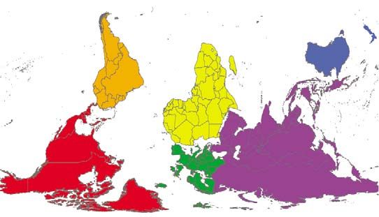
ware [Krzywinski, 2009] to create Figure 3. In Figure 3 the VWC is essentially a measure of how efficient, in terms of
links have the same color as their region of origin, and the water use, because of both climate (i.e., total evapotranspira-
link width is proportional to the volume of water exchanged. tion) and farming practices (i.e., crop yield), a country or region
For each region, we have also included the internal trade (i.e., is in producing a given crop or livestock product. For this
trade between countries of that region). This is represented by reason, it makes sense that regions with a relatively high VWC
links that originate and terminate in the same region. Trade (i.e., less efficient) import from regions with a comparative
between regions of a negligible size has been excluded from advantage in water use (i.e., more efficient).
Figure 3 for clarity. [22] From Figure 3 we notice that a regional network
[20] For the aggregate network from all water sources associated with the crop trade alone drives the aggregate
(e.g., Figure 3a), Asia, Europe, and Africa are net importers, (i.e., both crop and livestock commodities) regional trade
while Oceania, North America, and South America are net network. Note that Figures 3a and 3b are very similar in
exporters. The largest link is the export from North America both link connectivity and magnitude, while Figures 3c and
to Asia (over 94 × 109 m3 yr−1, almost 50% of the total 3d show differences when compared with Figure 3a. Thus,
export volume from North America), followed by the export even though the VWC of livestock products is higher than
from South America to Europe and Asia (71 × 109 m3 yr−1 the VWC of crop products (refer to Figure 1), the crop
and 50 × 109 m3 yr−1, respectively). Asia is the largest commodity trade drives the aggregated virtual water trade
importer of virtual water (267 × 109 m3 yr−1) and exhibits because of the fact that the volumes of crop commodities
a large internal trade (77% of exports are internal; refer to traded are much larger than volumes of livestock com-
Figure 3a). Although Europe imports only 137 × 109 m3 yr−1, modities. In fact, the regional crop trade network from green
it is the largest importer on a per capita basis, importing water (e.g., Figure 3e) drives the entire crop trade network
0.34 × 10⁹ m3 yr−1 per capita. (notice the similarities between Figures 3e and 3b, as well
[21] Asia transfers very large amounts of blue water from as those between Figures 3e and 3a), indicating that this
both crop and livestock products internally (see Figures 3g– regional network forms the foundation of the aggregate
3i); about 76% of blue water exports are internal in Asia. network from all water sources. This highlights the impor-
On the other hand, South America exports much more green tance of the underlying commodity trade network in driving
water than blue water. This difference is related to the the virtual water trade considered.
varying values of blue VWC for both crop and livestock
products between these two continents (refer to Figure 1). 3.2. Undirected Networks
Livestock and crop commodities produced in Asia utilize [23] In this section, we will focus our analysis on
much higher values of blue water (33% and 44% of total the symmetric, undirected networks, AU and WU. In these
virtual water content, respectively), while livestock and crop networks there are 184 active nodes (nations) and 4550
5 of 17W05520 KONAR ET AL.: NETWORK ANALYSIS OF GLOBAL VIRTUAL WATER W05520
Figure 3. Regional virtual water trade networks. Numbers are in billions of cubic meters of water per
year. The regional networks are broken down by source of virtual water and commodity trade. Regional
network of virtual water trade from (a) all sources of virtual water associated with trade in both crop
and livestock commodities, (b) all sources of virtual water associated with trade in crop commodities only,
(c) all sources of virtual water associated with trade in livestock commodities only, (d) green sources of
virtual water associated with trade in both crop and livestock commodities, (e) green sources of virtual
water associated with trade in crop commodities only, (f) green sources of virtual water associated with
trade in livestock commodities only, (g) blue sources of virtual water associated with trade in both crop
and livestock commodities, (h) blue sources of virtual water associated with trade in crop commodities
only, and (i) blue sources of virtual water associated with trade in livestock commodities only. The regional
map at the bottom provides a key to the color scheme of the regional trade networks. Note that the regional
acronyms follow those provided in the caption of Figure 1.
links. Element (i, j) of the adjacency matrix, A, is repre- In this symmetric matrix, ai,j = aj,i. Similarly, we constructed
sented by ai,j. The elements of the principal diagonal (ai,i) the symmetric weighted matrix WU, in which the elements
are set to 0 and elements off the principal diagonal (ai,j) wi,j are computed as the sum of the i → j and j → i flows
are equal to 1 when there is flow between nodes i and j. between the corresponding nations.
6 of 17W05520 KONAR ET AL.: NETWORK ANALYSIS OF GLOBAL VIRTUAL WATER W05520
Table 2. Country Rankings in 2000a trade volume of 20.2 × 10⁹ m3 yr−1, or 3.2% of the flow
Undirected Export Import
volume. In fact, in WU the United States is involved in 7 out
of the 10 largest links (refer to Table 4).
Rank k Country kout Country kin Country
[26] Node strength (s) is a measure of the weight of each
1 162 Netherlands 159 United States 97 United States node’s links. This value is calculated as si = Sj wi,j. Node
2 162 United States 158 Netherlands 94 UK strength values range from 50 × 103 to 183 × 109 m3 yr−1,
3
4
161
156
France
UK
154
152
France
Italy
89
87
Germany
Canada
with an average value of 6.79 × 10⁹ m3 yr−1. The nation that
5 154 Italy 150 UK 84 Netherlands trades the most virtual water (i.e., maximum strength) is the
6 152 Germany 149 Germany 82 France United States. Refer to Table 5 for the top 15 ranked nations
7 146 Belgium 142 Denmark 72 Saudi Arabia in terms of the volume of virtual water traded. This node
8 145 China 142 Belgium 69 Japan strength information provides a description of the centrality
9 144 Denmark 142 China 68 Spain
10 141 Canada 136 Canada 68 Belgium of nations according to the volume of virtual water traded.
11 133 Australia 129 Thailand 67 Switzerland [27] Graphs of undirected network properties are provided
12 133 Thailand 126 Australia 65 Italy in Figure 4. The cumulative degree distribution P(K > k)
13 126 Spain 124 Argentina 64 Australia is shown in Figure 4a. Many empirical analyses of real‐
14 125 Argentina 124 Brazil 64 Russia
15 125 Brazil 119 Spain 60 Hong Kong
world networks in the literature fit a power law to the tail
of P(K > k) [e.g., Barrat et al., 2004; Garlaschelli and
a
Top 15 positions according to node degree (k) statistics. Node degree is Loffredo, 2005; Kyriakopoulos et al., 2009]. However,
a measure of the number of trade partners of a given country, k is a measure
it is clear that here the simple exponential distribution, e.g.,
of the trade connections in the undirected network, kout counts the number
of export trade partners, and kin counts the number of import trade partners. P(K > x) = e−lx, as used by DeMontis et al. [2007], accu-
rately reflects the entirety of the data set (an exponential
distribution of hki is shown by the solid line in Figure 4a).
[24] A fundamental network property is the node degree Thus, the topology of the food trade networks exhibits a
(k), which measures the number of links of each node and is characteristic scale, different from the scale‐free behavior
defined as ki = Sj ai,j. Here the node degree is a measure of of other real‐world systems, such as those highlighted by
the number of trade partners of each nation. Node degree Barabási and Albert [1997]. The exponential parameter is
values range from 1 to 162, with an average value of hki = given by hki and is provided for each individual crop net-
49.46. The node degree is a first approximation of its work in Table 3.
topological centrality, which is an indication of its impor- [28] The cumulative distribution of node strength is
tance within the network. Two nations share the maximum shown in Figure 4b, where aa stretched exponential distri-
node degree value of 162: Netherlands and the United States bution, e.g., P(K > x) = e(−lx) , is compared with the data.
(see Table 2 for a ranking of the top 15 nations in terms The stretched exponential distribution parameter (a) for
of node degree). Node degree statistics for the aggregate the aggregate and individual crop networks is provided in
and individual crop networks are collected in Table 3. Table 3. This fat‐tailed distribution indicates that the volumes
[25] The volume of water traded globally is 625 × 109 m3 of virtual water traded by each nation are highly heteroge-
−1
yr (calculated as 1/2Si, j wi, j). The link weights range from neous. Thus, when the network weights are considered, a
77.72 m3 yr−1 to 29.2 × 10⁹ m3 yr−1 with a mean value of heavy‐tailed distribution is required to fit the data, unlike the
hwi = 137 × 106 m3 yr−1, indicative of high link weight exponential distribution fit to the node degrees. This implies
heterogeneity. The largest link in this network is between that the inclusion of network weights increases the heteroge-
the United States and Japan, with a virtual water trade neity of the system in a nontrivial way.
of 29.2 × 10⁹ m3 yr−1, which accounts for 4.7% of the entire [29] Probability distributions are frequently used in the
volume in the network. The second largest link is that natural sciences to explain data. Many environmental vari-
between the United States and Mexico, with a virtual water ables are distinctly asymmetric (i.e., non‐Gaussian) and
Table 3. Global Network Measures for Undirected Virtual Water Trade Networks
Crop
Symbol Barley Corn Rice Soy Wheat Beef Pork Poultry Aggregate
Active nodes N 175 178 175 175 178 172 169 168 184
Global flow (m3 yr−1) g 30.5 × 10⁹ 62.9 × 10⁹ 52.9 × 10⁹ 241 × 109 137 × 109 59.2 × 10⁹ 19.7 × 10⁹ 21.6 × 10⁹ 625 × 109
Number of links L 2257 1633 1860 1712 2664 1835 1675 1466 4550
Average degree hki 25.79 18.35 21.23 19.57 29.93 21.34 19.82 17.45 49.46
Maximum degree kmax 148 141 135 123 150 111 118 134 162
Average strength hsi 0.35 × 10⁹ 0.71 × 10⁹ 0.61 × 10⁹ 2.75 × 10⁹ 1.54 × 10⁹ 0.69 × 10⁹ 0.23 × 10⁹ 0.26 × 10⁹ 6.79 × 10⁹
(m3 yr−1)
Maximum strength smax 7.23 × 10⁹ 30.9 × 10⁹ 17.0 × 10⁹ 67.4 × 10⁹ 39.6 × 10⁹ 23.4 × 10⁹ 6.31 × 10⁹ 8.38 × 10⁹ 183 × 109
(m3 yr−1)
Clustering coefficient c 0.71 0.62 0.62 0.67 0.69 0.64 0.73 0.68 0.75
Clustering coefficient cER 0.15 0.10 0.12 0.11 0.17 0.12 0.12 0.10 0.27
random
Clustering coefficient cW 0.79 0.73 0.73 0.77 0.80 0.73 0.80 0.79 0.87
weighted
Stretched exponential g 0.28 0.22 0.22 0.2 0.24 0.35 0.3 0.24 0.28
parameter
7 of 17W05520 KONAR ET AL.: NETWORK ANALYSIS OF GLOBAL VIRTUAL WATER W05520
Table 4. Link Rankings in 2000a
Rank wU(i, j) (m3 yr−1) Country 1 Country 2 wD(i, j) (m3 yr−1) Country of Export Country of Import
9 9
1 29.2 × 10 United States Japan 29.2 × 10 United States Japan
2 20.2 × 10⁹ United States Mexico 19.2 × 10⁹ United States Mexico
3 14.5 × 10⁹ Canada United States 12.9 × 10⁹ Brazil Netherlands
4 12.9 × 10⁹ Brazil Netherlands 12.0 × 10⁹ United States China
5 12.5 × 10⁹ Argentina Brazil 11.9 × 10⁹ Argentina Brazil
6 12.0 × 10⁹ United States China 9.17 × 10⁹ United States Egypt
7 9.17 × 10⁹ United States Egypt 8.84 × 10⁹ Brazil France
8 8.90 × 10⁹ Brazil France 8.65 × 10⁹ United States Taiwan
9 8.65 × 10⁹ United States Taiwan 8.30 × 10⁹ Argentina China
10 8.30 × 10⁹ United States Korea 8.28 × 10⁹ United States Korea
11 8.30 × 10⁹ Argentina China 8.08 × 10⁹ Canada United States
12 7.79 × 10⁹ Australia Japan 7.79 × 10⁹ Australia Japan
13 7.68 × 10⁹ Kazakhstan Russia 7.61 × 10⁹ Kazakhstan Russia
14 7.49 × 10⁹ Argentina Spain 7.48 × 10⁹ Argentina Spain
15 6.88 × 10⁹ Argentina Italy 6.87 × 10⁹ Argentina Italy
a
Top 15 positions according to link weight (w): wU(i, j) represents element (i, j) in the weighted, undirected network and WD(i, j) represents element (i, j)
in the weighted, directed network. Note that we report which two countries share a particular link for wU(i, j). Since there is no direction in this network the
import‐export relationship does not exist.
important to properly quantify. For example, the Gamma [31] While node degree is the simplest proxy for cen-
distribution has been often used to explain precipitation trality, it is a local measure that does not provide any
data, with important applications in hydrologic models, such information about the importance of the node within the
as flooding or drought estimates [Wilks, 2006]. Similarly, global structure [Barthelemy, 2004]. A measure of centrality
we believe that the distributions of virtual water resources that takes into account the location of a node within the
presented here, influenced by both social and natural forces, entire network architecture is the betweenness centrality,
provide necessary statistical descriptions of the linked water which counts the fraction of shortest paths going through
and food system for water resource professionals. a given node. The betweenness centrality (B) is defined as
[30] To explore in further detail the relationship between Bu = Si,j ði;u;j Þ
ði;jÞ , where s(i, u, j) is the number of shortest
the node connectivity and weights, we plot the strength paths between nodes i and j that pass through node u, s(i, j)
of the nodes as a function of their degree in Figure 4c. is the total number of shortest paths between i and j, and the
We observe a power law relationship that follows the form sum is over all pairs i, j of nodes [Costa et al., 2007]. We
s(k) ∼ kb. The parameter b = 2.60 for the aggregate net- normalize B by (N − 1)(N − 2)/2 to maintain B 2 [0, 1] as
work and is provided in Table 6 for the individual crop suggested by Barthelemy [2004].
networks. This high b value indicates that there is a strong [32] B is an important measure of how important a node is
relationship between the volume of virtual water that each in terms of connecting other nodes in the network [Jackson,
nation trades and its number of trade partners. The node 2008]. The United States has the highest betweenness
strength grows faster than node degree, so the more trade centrality in the virtual water trade network, as shown in
connections a country has, the much more it is able to Table 7, highlighting its crucial role in the global struc-
participate in the exchange of virtual water in a highly ture. France and the United Kingdom also exhibit high
nonlinear way. betweenness centrality, ranking a close second and third,
Table 5. Country Rankings in 2000a
Undirected Export Import Import per Capita
Rank s (m3 yr−1) Country sout (m3 yr−1) Country sin (m3 yr−1) Country sin (capita−1) Country
9 9 9
1 183 × 10 United States 165 × 10 United States 52.1 × 10 Japan 1,954 United Arab Emirates
2 92.7 × 10⁹ Argentina 91.0 × 10⁹ Argentina 31.1 × 10⁹ China 1,885 Aruba
3 88.2 × 10⁹ Brazil 69.7 × 10⁹ Brazil 28.7 × 10⁹ Netherlands 1,802 Netherlands
4 52.5 × 10⁹ Japan 38.5 × 10⁹ Australia 24.2 × 10⁹ Korea 1,375 Cyprus
5 44.5 × 10⁹ China 34.5 × 10⁹ India 21.8 × 10⁹ Mexico 1,242 Qatar
6 40.7× 10⁹ Canada 32.7 × 10⁹ Canada 21.8 × 10⁹ Iran 1,158 Singapore
7 39.3 × 10⁹ Australia 20.0 × 10⁹ Thailand 19.5 × 10⁹ Italy 1,153 Hong Kong
8 37.7 × 10⁹ India 18.1 × 10⁹ France 19.3 × 10⁹ Egypt 1,127 Denmark
9 36.8 × 10⁹ Netherlands 13.4 × 10⁹ China 18.8 × 10⁹ Indonesia 1,097 Seychelles
10 35.5 × 10⁹ France 12.7 × 10⁹ Kazakhstan 18.5 × 10⁹ Brazil 974 Kuwait
11 30.0 × 10⁹ Thailand 11.7 × 10⁹ Germany 18.3 × 10⁹ Spain 927 Belgium
12 27.7 × 10⁹ Germany 11.2 × 10⁹ Pakistan 17.6 × 10⁹ Russia 826 Uruguay
13 25.0× 10⁹ Italy 8.65 × 10⁹ Denmark 17.5 × 10⁹ France 822 Netherlands Antilles
14 24.5 × 10⁹ Korea 8.06 × 10⁹ Netherlands 17.4 × 10⁹ United States 821 Malta
15 24.1 × 10⁹ Mexico 7.35 × 10⁹ Paraguay 16.1 × 10⁹ Germany 801 Israel
a
Top 15 positions according to node strength (s) statistics. Node strength is a measure of the weight of a given country; s is the volume of virtual water
traded by a country in the undirected network, sout measures the volume of virtual water exported by a country, and sin measures the volume of virtual water
imported by a country.
8 of 17W05520 KONAR ET AL.: NETWORK ANALYSIS OF GLOBAL VIRTUAL WATER W05520
Figure 4. Graphs for the undirected virtual water trade network. (a) The cumulative distribution of the
node degrees compared with an exponential distribution of parameter hki = 49.46. (b) The cumulative dis-
tribution of the node strength compared with a stretched exponential distribution of parameter a = 0.42.
(c) Node strength plotted against node degree exhibiting a power law relationship of the form s(k) ∼ kb, with
parameter b = 2.60. (d) Betweenness centrality of each node plotted against node degree exhibiting a power
law relationship of the form B(k) ∼ kg , with parameter g = 3.04. (e) Weighted (solid line) and unweighted
(dashed line) average nearest‐neighbor degree as a function of node degree. (f) Weighted (solid line) and
unweighted (dashed line) clustering coefficient as a function of node degree.
respectively, with values closely trailing the United States. degree (knn); knn measures the affinity of a given node to
The United States, France, and the United Kingdom all connect to high‐ or low‐degree neighbors. The unweighted
exhibit B values that are approximately 3 times higher definition of knn is given by [Pastor‐Satorras et al., 2001]
than other highly ranked countries, such as Spain and India
(e.g., ranked 14th and 15th out of 184 countries, respec- 1 X
knni ¼ kj ; ð4Þ
tively). B versus node degree follows a power law distri- ki j2V ðiÞ
bution of the form B(k) ∼ kg , shown in Figure 4d. The
parameter g = 3.04 for the aggregate network, and it is where j 2 V(i) indicates the j neighbors of node i. Thus, knni
provided in Table 6 for individual crop networks. identifies all nodes in the neighborhood of i (i.e., connected
[33] We next consider the network correlation structure, to node i), sums their respective node degrees, then nor-
typically quantified using the average nearest‐neighbor malizes by the node degree of node i.
Table 6. Parameters for Each Network
Crop
Symbol Barley Corn Rice Soy Wheat Beef Pork Poultry Aggregate
s versus k b 2.37 2.28 1.87 2.68 2.15 2.41 2.41 2.07 2.60
sin versus kin b in 2.16 2.71 2.02 3.32 2.12 2.63 2.75 2.20 3.05
sout versus kout bout 2.21 1.71 1.76 1.90 1.75 2.10 1.91 1.91 1.93
B versus k g 2.76 2.58 2.61 2.60 2.70 2.56 2.79 2.31 3.04
9 of 17W05520 KONAR ET AL.: NETWORK ANALYSIS OF GLOBAL VIRTUAL WATER W05520
Table 7. Country Rankings in 2000a ference between kW nn and knn grows with increasing k, indi-
Rank B Country
cating that highly connected nations are more likely to
be connected when link flows are considered. In sharp con-
1 0.093 United States trast to topological disassortativity, we observe an affinity
2 0.092 France between nations of high degree which exchange large
3 0.091 United Kingdom
4 0.078 Netherlands volumes of virtual water. In other words, large weights
5 0.068 Italy preferentially connect hubs, while nodes of a smaller degree
6 0.065 Germany are connected via smaller weights.
7 0.063 China [37] The clustering coefficient allows us to study the
8 0.053 Denmark
9 0.052 Australia tendency of nations in the network to form tightly connected
10 0.049 Canada groups. The clustering coefficient is defined as
11 0.045 Thailand
12 0.044 Japan 2ei
13 0.038 South Africa ci ¼ ; ð6Þ
14 0.034 Spain ki ðki 1Þ
15 0.032 India
a
where ei is the number of links between the ki neighbors of
Top 15 positions according to node betweenness centrality (B) statistics.
Node betweenness centrality measures the centrality of each node in terms
node i and ki(ki − 1)/2 is the maximum possible number of
of its location within the global network architecture. links existing between the ki neighbors of i [Boguna and
Pastor‐Satorras,2003; DeMontis et al., 2007]. In other
words, ci counts the number of closed triangles formed in
[34] The behavior of knn as a function of k allows us to the neighborhood of node i. This value measures the local
determine whether or not the network exhibits degree cor- cohesiveness of the network and 2 [0,1]. Values of ci = 0
relations. If knn increases with k, the network is referred to as indicate that the neighbors of i are not connected at all,
assortative, and nodes with a high degree tend to connect to while values of ci = 1 correspond to the case in which all
other nodes with a high degree, while nodes with a low the neighbors of i are themselves connected. The average
degree tend to connect to nodes with a low degree. How- clustering coefficient of the virtual water trade network
ever, if knn is a decreasing function of k, then the network is 0.75, much higher than that of a random network (cER)
is disassortative, indicating that nodes of high degree tend with the same number of links and nodes (refer to Table 3;
to connect to neighbors with low degree and nodes of low cER = 0.27), where cER = L/N (N − 1) [Bollobás, 1985].
degree tend to connect to others with a high degree. In [38] The definition of ci has been extended to weighted
Figure 4e, we see that for the undirected case, knn decreases networks by Barrat et al. [2004] and is defined as
with k, suggesting that the global virtual water trade network
is disassortative, typical of technological, biological, and 1 X wij þ wih
transportation networks [Newman, 2003; Costa et al., 2007]. cW
i ¼ aij aih ajh ; ð7Þ
si ðki 1Þ j;h 2
In other words, when we consider only network topology,
nations of high degree tend to be connected to nations that
have a low degree. This disassortative behavior indicates where 1/si(ki − 1) is a normalization factor to maintain cWi 2
that the network exhibits a global architecture in which [0,1]. Using this definition, the relative weight of closed
hubs (i.e., nations with high degree) provide the connec- triangles in the neighborhood of node i is considered. Here
tivity for the peripheral nations with small degree [DeMontis the mean weighted clustering coefficient is greater than the
et al., 2007]. unweighted version (refer to Table 3; cW = 0.87 > c = 0.75),
[35] The definition of knn has been extended for weighted indicating that cohesiveness is more likely when link weights
networks by [Barrat et al., 2004] are taken into account.
[39] We plot c and cW as a function of node degree in
W 1 X Figure 4f; c decreases with increasing values of k. This
knn ¼ wij kj ; ð5Þ
i
si j2V ðiÞ behavior indicates that nations with a low degree belong to
tightly connected groups of nations, while nations with
where, as in the unweighted definition, j 2 V(i) indicates high degree connect otherwise disconnected portions of the
the j neighbors of node i. The value of the links between network [DeMontis et al., 2007]. Here, as with the nearest‐
node i and its neighbors (wij) is now accounted for, in neighbor degree, the introduction of network weights
addition to the node degree of the neighbors, before nor- destroys the correlation structure, such that cW (k) is approx-
malizing by the node strength of i rather than the node imately constant and cW (k) > c (k) over the whole range
degree of i as in the unweighted definition. This definition of degrees.
measures the affinity of a node to connect with low‐ or [40] In summary, the disassortative behavior of the aver-
high‐degree neighbors on the basis of the magnitude of the age nearest‐neighbor degree and the clustering coefficient
actual interactions. If links with large edges point to breaks down with the inclusion of network weights (refer to
neighbors with large degree, then kW Figures 4e and 4f). The accumulation of weight on highly
nn(k) > knn (k). However,
kW connected nations destroys the disassortative behavior,
nn(k) < knn if links with large weights point to neighbors
with low degree [Barrat et al., 2004]. suggesting the existence of the “weighted rich club” phe-
[36] Both knn and kW nomenon [DeMontis et al., 2007]. This phenomenon occurs
nn are plotted against k in Figure 4e.
Note that the disassortative structure of the unweighted knn when prominent elements in a system engage in stronger
breaks down when weights are taken into account (compare or weaker interactions among themselves than expected by
the solid line with the dashed line in Figure 4e). The dif- pure chance [Opsahl et al., 2008]. Thus, when we utilize
10 of 17W05520 KONAR ET AL.: NETWORK ANALYSIS OF GLOBAL VIRTUAL WATER W05520
information on the volume of virtual water embedded in [45] The link weights in the directed network range from
each trade link, we obtain additional insights into the net- 77.72 m3 yr−1 to 29.2 × 10⁹ m3 yr−1, with a mean value of
work organizing principles. 104 × 106 m3 yr−1. The largest link weight in WD is United
States → Japan, with a value of 29.2 × 10⁹ m3 yr−1, or 4.7%
3.3. Directed Networks of the network’s total flow. The United States and Japan
[41] We now consider the direction of trade in the network have been shown to be important nations in the virtual water
analysis. In this section we focus our attention on the AD literature [Hoekstra and Hung, 2005; Hoekstra and Chapagain,
and WD networks. Direction is an important characteristic 2008], which this study confirms. The second largest link in
because the virtual water trade network is not symmetric, the network is United States → Mexico, with a value of
which means that information on the network structure is 20.2 × 10⁹ m3 yr−1, which represents 3.1% of the global flow.
lost when we symmetrize the network for the undirected Even though the links between Japan and the United States
analysis. In these directed networks there are 151 nations and the United States and Mexico were also the largest links
that export, 166 nations that import, and 6033 links. There in the undirected network, we are now able to distinguish
are some nations that either import or export but not both flow direction. The link between Canada and the United
(e.g., Qatar does not export but only imports). The global States is the third largest link in the symmetric network (with
volume of water traded in the directed network is equivalent a value of 14.5 × 10⁹ m3 yr−1) but the 11th largest link in the
to that of the undirected network at 625 × 109 m3 yr−1. Our directed network. In the directed network, the link Canada →
global flow volume is slightly greater than that found by United States accounts for 8.08 × 10⁹ m3 yr−1 (see Table 4), a
Hanasaki et al. [2010] (i.e., 625 × 109 m3 yr−1 compared with whole order of magnitude less, because of the fact that trade
545 × 109 m3 yr−1) because of the fact that we utilize both United States → Canada is also relatively large (valued at
the import and export trade data from the FAO. 6.46 × 10⁹ m3 yr−1). This example illustrates that information
[42] As in the undirected case, ai,j represents element i, j is lost through network symmetrization.
of the adjacency matrix. The elements of the principal [46] Differences between our virtual water flow volumes
diagonal (ai,i) are set to 0 and elements off the principal and other values reported in the literature can be attributed
diagonal (ai,j) are equal to 1 when there is flow i → j. to differences in VWC and the agricultural commodities
However, unlike in the symmetric case, element ai,j ≠ aj,i. considered, though major differences are mainly due to
In the weighted matrix (WU), the elements (wi,j) represent differences in the underlying commodities. For example, we
the flows i → j between the corresponding nations. Note that calculate the total virtual water import of the United States
wi,j is no longer equivalent to wj,i. due to crop commodities to be 8.21 × 10⁹ m3 yr−1. However,
[43] We now consider the out‐ and in‐node degrees, Hoekstra and Hung [2005], whose study is based on 38 crop
which provide additional information on the heterogeneity commodities, determine that the United States imports
of the network connectivity. The out‐node degree (kouti = 29.3 × 10⁹ m3 yr−1, while Hoekstra and Chapagain [2008],
Sj ai, j) values range from 0 to 159 with a mean value of in a study based on 285 crop commodities, calculate the
32.79; the in‐node degree (kini = Sj aj,i) values range from same value at 73.1 × 10⁹ m3 yr−1. It makes sense that we would
0 to 97 with a mean value of 32.79. We rank each nation obtain a much lower value than Hoekstra and Chapagain
according to its degree for both the undirected and directed [2008] for the import of crops to the United States, since
network in Table 2. Note that the United States has the this wealthy nation likely imports many specialty crops
highest kin and kout values. This is striking, since Netherlands that are not included in our analysis, since we focus on
and the United States tie for the highest rank in the undi- staple crops. Our values compare relatively well for other
rected network. This indicates that although the United flows.
States has the most import and export trading partners, there [47] For weighted, directed networks the natural gener-
is significant overlap in these trading partners such that alization of the out and in degree of a node is the out‐ and
when AD is symmetrized, Netherlands gains the most links. in‐node strength, where souti = Sj wi, j and sini = Sj wj,i,
Netherlands is a strategic harbor in Europe, so this diversity respectively. The import volumes (sin) range from 0 m3 yr−1
in trading partners makes sense. to 52.1 × 10⁹ m3 yr−1, with a mean value of 3.40 × 10⁹ m3
[44] The cumulative distributions of the out‐ and in‐node yr−1; the export volumes (sout) range from 0 m3 yr−1 to 165 ×
degrees of AD are shown in Figures 5a and 5b. We compare 109 m3 yr−1, also with a mean value of 3.40 × 10⁹ m3 yr−1.
an exponential distribution of parameter hkouti to the out‐ The cumulative distributions of the in‐ and out‐node
node degrees and parameter hkini to the in‐node degrees, strengths are compared with the stretched exponential dis-
as we did for the undirected network. Note that the in‐node tribution in Figures 5c and 5d. As in the undirected network,
degree does not follow an exponential distribution, while the stretched exponential distribution provides an excellent fit
the out‐node degree distribution does appear to follow an to the directed node strength distributions. This indicates that
exponential. The tail of kout is fatter than the tail of kin. The the high node strength heterogeneity is maintained when
tail of kin actually drops off quicker than an exponential direction is taken into account.
distribution (refer to the tails in Figures 5a and 5b). This [48] We rank nations according to their strength in
indicates that it is frequent that countries will export to many Table 5. Table 5 provides additional insight into the node
trade partners, while they tend to import from just a few strength heterogeneity that is lost by symmetrizing the net-
trade partners. This makes sense, since if a country is effi- work to create the undirected network. For example, Japan
cient at producing a given commodity, then it will likely imports the largest volume of virtual water but ranks 52nd
export it to many partners. However, if a nation must import in terms of export volume. However, when we symmetrize
a given commodity, it will likely be able to meet its demand the directed network on the basis of the sum of trade
for this commodity in a few trade relationships. between any two nations, we lose this information and Japan
becomes the fourth‐ranked nation in terms of node strength.
11 of 17W05520 KONAR ET AL.: NETWORK ANALYSIS OF GLOBAL VIRTUAL WATER W05520
Figure 5. Graphs for the directed virtual water trade network. (a) The cumulative distribution of the out‐
node degrees compared with an exponential distribution of parameter hkouti = 32.79. (b) The cumulative
distribution of the in‐node degrees compared with an exponential distribution of parameter hkini = 32.79.
(c) The cumulative distribution of the out‐node strengths compared with a stretched exponential distribu-
tion of parameter aout = 0.28. (d) The cumulative distribution of the in‐node strengths compared with a
stretched exponential distribution of parameter ain = 0.48. (e) Out‐node strength plotted against out‐
node degree exhibiting a power law relationship of the form sout(kout) ∼ kbout
out , where parameter b out =
1.93. (f) In‐node strength plotted against in‐node degree exhibiting a power law relationship of the form
sin(kin) ∼ kbin
in , where parameter b in = 3.05.
Similarly, Australia is the fourth largest global exporter of water and trade connections remains when direction is taken
virtual water but comes in 87th in terms of import and 7th into account. In fact, the value of b in is larger than the value of
in the undirected case. When we analyze the volume of b, which indicates that the relationship between sin and kin is
virtual water that each country imports on a per capita even stronger than the relationship between the undirected
basis, the rankings change dramatically. The United Arab strength and node degree, particularly for the soy network,
Emirates is the largest importer per capita. Most of the where bin = 3.32.
nations that import a lot of virtual water on a per capita basis [50] Thus, as nations increase the number of countries that
are either island nations or wealthy countries with a relatively they import from, they increase the volume of virtual water
small population. Importantly, many of these countries are obtained at an even greater rate. This finding has important
extremely arid (i.e., United Arab Emirates, Qatar, Kuwait, policy implications, indicating that increasing the number
and Israel) or lack sufficient water and land resources for of import trade partners is an efficient way for countries to
agricultural production (i.e., Aruba, Cyprus, Singapore, Hong improve access to water resources. In our related paper
Kong, Seychelles, Netherlands Antilles, and Malta). [Suweis et al., 2011], we develop a model of global virtual
[49] As in the undirected network analysis, we plot water trade with predictive capabilities, in which we detail
the strength of the nodes as a function of their degree in the controls on the network structure. We find that both
Figures 5e and 5f. Similarly, we observe a power law rela- economic and climatologic factors are necessary to capture
tionship that follows the form sin (kin) ∼ kbin
in and sout (kout) ∼ the global properties. In particular, the gross domestic
kbout
out . The parameter b in is 3.05, and the parameter bout product of each nation is used to model the connectivity
is 1.94 for the aggregate network and is provided in Table 6 structure, while the rainfall on agricultural area is necessary
for the individual crop networks. These high b values indi- to determine the weighted network properties (i.e., the
cate that the strong relationship between the volume of virtual volumes of virtual water). Thus, both the economy and
12 of 17You can also read