Manual Computational Anatomy Toolbox - CAT12 - Structural ...
←
→
Page content transcription
If your browser does not render page correctly, please read the page content below
Manual
           Computational Anatomy Toolbox - CAT12

Quick start guide                                                2

Version information                                              4

Introduction and Overview                                        7

Getting Started                                                  7
       download and Installation                                7
       starting the toolbox                                     7
       basic vbm analysis (overview)                            8

Basic VBM Analysis (detailed description)                       10
   Preprocessing Data                                           11
       First Module: Segment Data                               11
       Second Module: Display one slice for all images          12
       Third Module: Estimate Total Intracranial Volume (TIV)   13
       Fourth Module: Check sample homogeneity                  13
       Fifth Module: Smooth                                     15
   Building the Statistical Model                               16
       Two-sample T-Test                                        17
       Full Factorial Model (for a 2x2 Anova)                   18
       Multiple Regression (Linear)                             19
       Multiple Regression (Polynomial)                         20
       Full Factorial Model (Interaction)                       21
       Full Factorial Model (Polynomial Interaction)            22
       Estimating the Statistical Model                         23
       Checking for Design Orthogonality                        23
       Defining Contrasts                                       25

                                                       1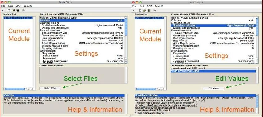
Special Cases                                                        30
   CAT12 for longitudinal data                                       30
       Optional Change of Parameters for Preprocessing               32
       Preprocessing of Longitudinal Data                            32
       Statistical Analysis of Longitudinal Data in One Group        33
       Statistical Analysis of Longitudinal Data in Two Groups       34
   Adapting the CAT12 workflow for unusual populations               38
       Customized Tissue Probability Maps                            38
       Customized DARTEL-template                                    39

Other variants of computational morphometry                          42
   Deformation-based morphometry (DBM)                               42
   Surface-based morphometry (SBM)                                   43
   Region of interest (ROI) analysis                                 46

Additional information on native, normalized and modulated volumes   47

Naming convention of output files                                    49

Calling CAT from the UNIX command line                               51

Technical information                                                51

                                                     2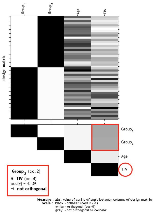
Quick start guide
VBM data
● Segment data using defaults (use Segment Longitudinal Data for longitudinal data).
● Estimate Total Intracranial Volume (TIV) to correct for different head size and volume.
● Check the data quality with Check Sample Homogeneity for VBM data (optionally consider TIV
and age as nuisance variable).
● Smooth data (recommended start value 8mm1).
● Specify 2nd-level model and check for design orthogonality and sample homogeneity:
o Use "Full factorial" for cross-sectional data.
o Use "Flexible factorial" for longitudinal data.
o Use TIV as covariate (confound) to correct different brain sizes and select centering
with overall mean.
o Select threshold masking with an absolute value of 0.1. This threshold can
ultimately be increased to 0.2 or even 0.25.
o If you find a considerable correlation between TIV and any other parameter of
interest it is advisable to use global scaling with TIV. For more information, refer to
the section “Building the statistical model”.
● Estimate model.
● Optionally, Transform SPM-maps to (log-scaled) p-maps or correlation maps and apply
thresholds.
● Optionally, you can try Threshold-Free Cluster Enhancement (TFCE) with the SPM.mat file of a
previously estimated statistical design.
● Optionally, Overlay Selected Slices. If you are using log-p scaled maps from Transform
SPM-maps without thresholds, use the following values as the lower range for the colormap
for the thresholding: 1.3 (P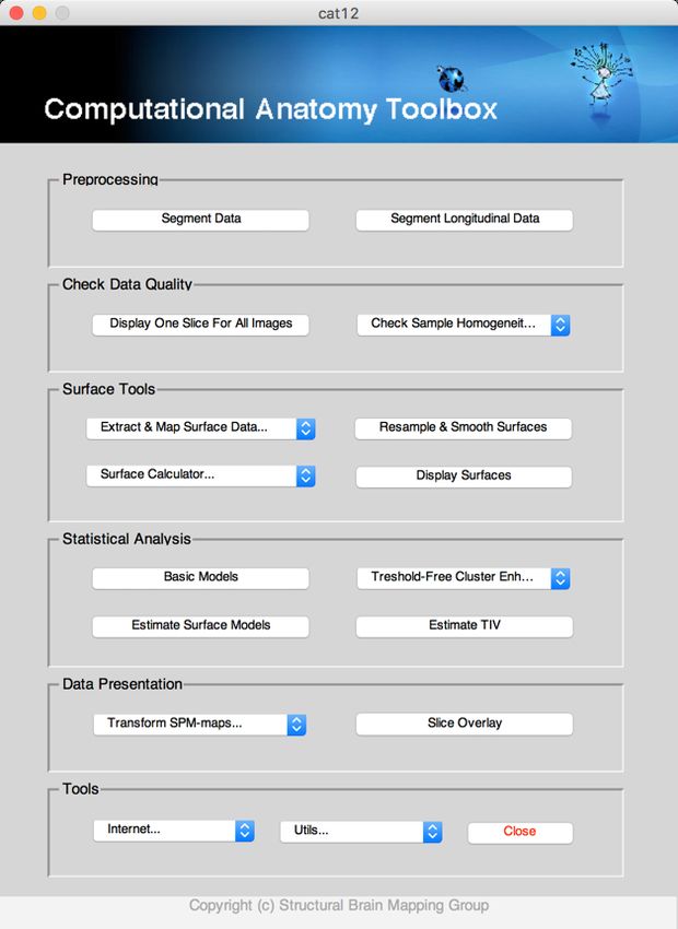
o It is not necessary to use threshold masking.
o If you find a considerable correlation between a nuisance parameter and any other
parameter of interest it is advisable to use global scaling with that parameter. For
more information, refer to the section “Building the statistical model”.
● Estimate Surface Model for (merged) hemispheres.
● Optionally, Transform SPM-maps to (log-scaled) p-maps or correlation maps and apply
thresholds.
● Optionally, you can try Threshold-Free Cluster Enhancement (TFCE) with the SPM.mat file of a
previously estimated statistical design.
● Optionally, Display Surface Results for both hemispheres. Select the results (preferably saved
as log-p maps with “Transform and threshold SPM-surfaces”) to display rendering views of
your results.
● Optionally Extract ROI-based Surface Values such as thickness, gyrification or fractal
dimension to provide ROI analysis.
● Optionally, estimate results for ROI analysis using Analyze ROIs. Here, the SPM.mat file of a
previously estimated statistical design is used. For more information, see the online
help “Atlas creation and ROI based analysis”.
Errors during preprocessing
Please use the Report Error function if any errors during preprocessing occurred. You first have to
select the "err" directory, which is located in the folder of the failed record and finally the
specified zip-file should be attached manually in the mail.
Additional options
Additional parameters and options are displayed in the CAT12 expert mode. Please note that this
mode is for experienced users only.
1
Note to filter sizes for Gaussian smoothing
Due to the high accuracy of the spatial registration approaches used in CAT12 you can also try to
use smaller filter sizes of only a few millimeter. However, for very small filter sizes or even no
filtering you have to apply a non-parametric permutation test such as the TFCE-statistics.
Please also note that for the analysis of cortical folding measures such as gyrification or cortical
complexity the filter sizes have to be larger (i.e. in the range of 15-25mm). This is due to the
underlying nature of this measure that reflects contributions from both sulci as well as gyri.
Therefore, the filter size should exceed the distance between a gyral crown and a sulcal fundus.
4Version information
Preprocessing should remain unaffected until the next minor version number. A new processing of
your data is not necessary if the minor version number of CAT12 remains unchanged.
Changes in version CAT12.6 (1444)
● Changes in preprocessing pipeline (which affects your results compared to CAT12.5)
o Two main parts of the preprocessing of CAT12 were largely updated: (1) Incorrect
estimates of the initial affine registration were found to be critical for all subsequent
preprocessing steps and mainly concerned skull-stripping and tissue segmentation.
This was a particular problem in brains of older people or children, where the
thickness of the skull differs from that of the template. The new estimate of the initial
affine registration should now be more robust. In the CAT report the registered
contour of the skull and the brain is now overlayed onto the image to allow for easier
quality control. (2) Skull-stripping now uses a new adaptive probability region-growing
(APRG) approach, which should also be more robust. APRG refines the probability
maps of the SPM approach by region-growing techniques of the gcut approach with a
final surface-based optimization strategy. This is currently the method with the most
accurate and reliable results.
o The longitudinal pipeline should now be more sensitive also for detection of effects
over longer time periods with VBM (ROI and SBM approaches are not affected by the
length of the period). In earlier versions, the average image was used to estimate the
spatial registration parameters for all time points. Sometimes this average image was
not as accurate if the images of a subject were too different (e.g. due to large
ventricular changes). Now, we rather use the average of spatial registration
parameters (i.e. deformations) of all time points, which makes the approach more
robust for longer periods of time. However, the SPM12 Longitudinal Toolbox can be a
good alternative for longer periods of time if you want to analyze your data voxel by
voxel. Surface-based preprocessing and also the ROI estimates in CAT12 are not
affected by the potentially lower sensitivity to larger changes, as the realigned images
are used independently to create cortical surfaces, thickness, or ROI estimates.
● Important new features
o CAT report now additionally plots the contour of the registered skull and brain and the
central surface onto the image and visualizes the result of skull-stripping. “Display
Surface Results” is largely updated.
o Parallelization options in CAT12 now enable subsequent batch jobs and are also
supported for longitudinal preprocessing.
Changes in version CAT12.5 (1355)
● Changes in preprocessing pipeline (which affects your results compared to CAT12.3)
o Detection of white matter hyperintensities (WMHs) is updated and again enabled by
default.
o The default internal interpolation setting is now "Fixed 1 mm" and offers a good
trade-off between optimal quality and preprocessing time and memory demands.
Standard structural data with a voxel resolution around 1 mm or even data with high
in-plane resolution and large slice thickness (e.g. 0.5x0.5x1.5 mm) will benefit from this
setting. If you have higher native resolutions the highres option "Fixed 0.8 mm" will
5sometimes offer slightly better preprocessing quality with an increase of preprocessing
time and memory demands.
● Important new features
o CAT12 can now deal with lesions that have to be set to “0” in your image using the
Stroke Lesion Correction (SLC) in expert mode. These lesion areas are not used for
segmentation or spatial registration, thus these preprocessing steps should be almost
unaffected.
Changes in version CAT12.4 (1342)
● This version had some severe errors in spatial registration which affected all spatially
registered data and should not be used anymore.
Changes in version CAT12.3 (1310)
● Changes in preprocessing pipeline (which affects your results compared to CAT12.2)
o Skull-stripping is again slightly changed and the SPM approach is now used as default.
The SPM approach works quite stable for the majority of data. However, in some rare
cases parts of GM (i.e. in frontal lobe) might be cut. If this happens the GCUT approach
is a good alternative.
o Spatial adaptive non-local mean (SANLM) filter is again called as very first step because
noise estimation and de-noising works best for original (non-interpolated) data.
o Detection of white matter hyperintensities (WMHs) is currently disabled by default,
because of unreliable results for some data.
● Important new features
o Cobra atlas has been largely extended and updated.
Changes in version CAT12.2 (1290)
● Changes in preprocessing pipeline (which affects your results compared to CAT12.1)
o Skull-stripping now additionally uses SPM12 segmentations by default: The default
gcut approach in CAT12.1 removed too much of the surrounding (extracranial) CSF,
which led to a slight underestimation of TIV for atrophied brains. The skull-stripping
approach based on the SPM12 segmentations prevents this through a more
conservative approach. However, sometimes parts of the meninges (i.e. dura mater) or
other non-brain parts still remain in the GM segmentation. By combining both
approaches a more reliable skull-stripping is achieved.
o More reliable estimation of TIV: The changed skull-stripping also affects estimation of
TIV, which is now more reliable, especially for atrophied brains.
● Important new features
o Automatic check for design orthogonality and sample homogeneity using SPM.mat in
Basic Models
o Added equi-volume model by Bok and multi-save option for mapping native volumes
to individual surfaces.
o Added Local-Global Intrinsic Functional Connectivity parcellation by Schaefer et al. for
resting-state fMRI data.
6Introduction and Overview
This manual is intended to help any user to perform a computational anatomy analysis using the
CAT12 Toolbox. Although it mainly focuses on voxel-based morphometry (VBM) other variants of
computational analysis such as deformation-based morphometry (DBM), surface-based
morphometry (SBM), and region of interest (ROI) morphometric analysis are also presented and
can be applied with few changes.
Basically, the manual can be divided into four main sections:
● Naturally, a quick guide of how to get started is given at the beginning. This section provides
information about downloading and installing the software and starting the Toolbox. In
addition, a brief overview of the steps of a VBM analysis is given.
● This is followed by a detailed description of a basic VBM analysis that guides the user
step-by-step through the entire process – from preprocessing to contrast selection. This
description should provide all the information necessary to successfully analyze most studies.
● There are some specific cases of VBM analyses, for which the basic analysis workflow needs to
be adapted. These cases are longitudinal studies and studies in children or special patient
populations. Relevant changes to a basic VBM analysis are described here and how to apply
these changes. It is important that only the changes are described – steps such as quality
control or smoothing are the same as those described in the basic analysis and not repeated a
second time.
● The guide concludes with information about native, normalized and modulated volumes that
determine how the results can be interpreted. In addition, an overview of the naming
conventions used and technical information is given.
Getting Started
DOWNLOAD AND INSTALLATION
● The CAT12 Toolbox runs within SPM12. That is, SPM12 must be installed and added to your
Matlab search path before the CAT12 Toolbox can be installed (see
http://www.fil.ion.ucl.ac.uk/spm/ and http://en.wikibooks.org/wiki/SPM).
● Download (http://dbm.neuro.uni-jena.de/cat12/) and unzip the CAT12 Toolbox. You will get a
folder named “cat12”, which contains various Matlab files and compiled scripts. Copy the
folder “cat12” into the SPM12 “toolbox” folder.
7STARTING THE TOOLBOX
● Start Matlab
● Start SPM12 (i.e., type “spm fmri”)
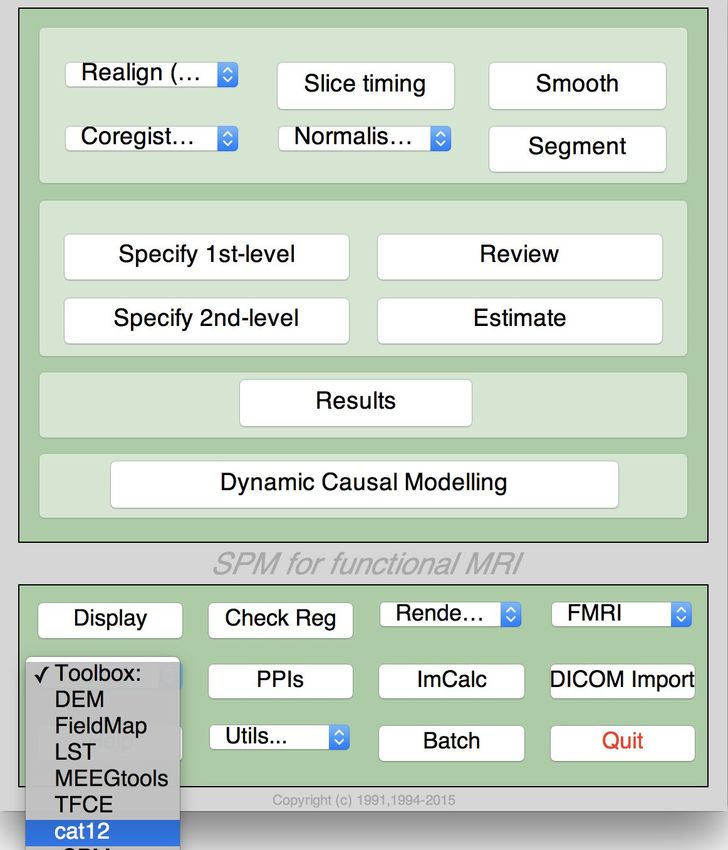
● Select “cat12” from the SPM menu (see Figure 1). You will find the drop-down menu between
the “Display” and the “Help” button (you can also call the Toolbox directly by typing “cat12”
on the Matlab command line). This will open the CAT12 Toolbox as additional window (Fig. 2).
Figure 1: SPM menu Figure 2: CAT12 Window
BASIC VBM ANALYSIS (OVERVIEW)
The CAT12 Toolbox comes with different modules, which may be used for an analysis. Usually, a
VBM analysis comprises the following steps
(a) Preprocessing:
1. T1 images are normalized to a template space and segmented into gray matter (GM),
white matter (WM) and cerebrospinal fluid (CSF). The preprocessing parameters can be
adjusted via the module “Segment Data”.
2. After the preprocessing is finished, a quality check is highly recommended. This can be
achieved via the modules “Display one slice for all images” and “Check sample
homogeneity”. Both options are located in the CAT12 window under “Check Data Quality”.
Furthermore, quality parameters are estimated and saved in xml-files for each data set
8during preprocessing. These quality parameters are also printed on the report PDF-page
and can be additionally used in the module “Check sample homogeneity”.
3. Before entering the GM images into a statistical model, image data need to be smoothed.
Of note, this step is not implemented into the CAT12 Toolbox but achieved via the
standard SPM module “Smooth”.
(b) Statistical analysis:
4. The smoothed GM images are entered into a statistical analysis. This requires building a
statistical model (e.g. T-Tests, ANOVAs, multiple regressions). This is done by the standard
SPM modules “Specify 2nd Level” or “Basic Models” in the CAT12 window covering the
same function.
5. The statistical model is estimated. This is done with the standard SPM module “Estimate”
(except for surface-based data where the function “Estimate Surface Models” should be
used instead).
6. If you have used total intracranial volume (TIV) as confound in your model to correct for
different brain sizes it is necessary to check whether TIV reveals a considerable correlation
with any other parameter of interest and rather use global scaling as alternative approach.
7. After estimating the statistical model, contrasts are defined to get the results of the
analysis. This is done with the standard SPM module “Results”.
The sequence of “preprocessing → quality check → smoothing → statistical analysis” remains
the same for every VBM analysis, even when different steps are adapted (see “special cases”).
A few words about the Batch Editor…
− As soon as you select a module from the CAT12 Toolbox menu, a new window (the Batch
Editor) will open. The Batch Editor is the environment where you will set up your analysis
(see Figure 3). For example, an “Figure 3: The Batch Editor is the environment where the analysis is set up. Left: For all settings marked with “
Basic VBM Analysis (detailed description)
Preprocessing Data

FIRST MODULE: SEGMENT DATA

Please note that additional parameters for expert users are displayed in the GUI if you set the
option cat.extopts.expertgui to “1” in cat_defaults.m or call cat12 by:
cat12(‘expert’)

CAT12 → Preprocessing → Segment Data

       Parameters:

           o Volumes
selected (e.g. for children data) that was created using the DARTEL toolbox. For
more information on the necessary steps, see the section "Customized DARTEL
Template".
o Writing options → [use defaults or modify]
- For GM, and WM image volumes see at the end of the document: “Additional
information on native, normalized and modulated normalized volumes”. Note:
The default option “Modulated normalized” results in an analysis of relative
differences in regional GM volume, that have to be corrected for individual
brain size in the statistical analysis using total intracranial volume (TIV).
- A Bias, noise and globally intensity corrected T1 image, in which MRI
inhomogeneities and noise are removed and intensities are globally
normalized, can be written in normalized space. This is useful for quality
control and also to create an average image of all normalized T1 images to
display / overlay the results. Note: For a basic VBM analysis use the defaults.
- A partial volume effect (PVE) label image volume can also be written in
normalized or native space or as a DARTEL export file. This is useful for quality
control and also for future applications using this image to reconstruct
surfaces. Note: For a basic VBM analysis use the defaults.
- The Jacobian determinant for each voxel can be written in normalized space.
This information can be used to do a Deformation-Based Morphometry (DBM)
analysis. Note: For a basic VBM analysis this is not needed.
- Finally, deformation fields can be written. This option is useful to re-apply
normalization parameters to other co-registered images (e.g. fMRI or DTI data).
Note: For a basic VBM analysis this is not needed.
Note: If the segmentation fails, this is often due to an unsuccessful initial spatial registration. In
this case, you can try to set the origin (anterior commissure) in the Display tool. Place the cursor
roughly on the anterior commissure and press “Set Origin” The now displayed correction in the
coordinates can be applied to the image with the button “Reorient”. This procedure must be
repeated for each data set individually.
SECOND MODULE: DISPLAY ONE SLICE FOR ALL IMAGES
CAT12 → Check data quality → Display one slice for all images
Parameters:
o Sample datatemplates → T1”). Adjust if necessary using “Display” from the SPM main
menu.
o Proportional scaling →[use defaults or modify]
- Check “yes”, if you display T1 volumes.
o Spatial orientation
o Show slice in mm → [use defaults or modify]
- This module displays horizontal slices. This default setting provides a good
overview.
THIRD MODULE: ESTIMATE TOTAL INTRACRANIAL VOLUME (TIV)
CAT12 → Statistical Analysis → Estimate TIV
Parameters:
o XML filesmatrices. Thus, it will help identifying outliers. Any outlier should be carefully
inspected for artifacts or pre-processing errors using “Check worst data” in the
GUI. If you specify different samples the mean correlation is displayed in
separate boxplots for each sample.
o Load quality measures (optional) → [optionally select xml-files with quality
measures]
- Optionally select the xml-files that are saved for each data set. These files
contain useful information about some estimated quality measures that can be
also used for checking sample homogeneity. Please note, that the order of the
xml-files must be the same as the other data files.
o Separation in mm → [use defaults or modify]
- To speed up calculations you can define that correlation is estimated only
every x voxel. Smaller values give slightly more accurate correlation, but are
much slower.
o Nuisance → [enter nuisance variables if applicable]
- For each nuisance variable which you want to remove from the data prior to
calculating the correlation, select “New: Nuisance” and enter a vector with the
respective variable for each subject (e.g. age in years). All variables have to be
entered in the same order as the respective volumes. You can also type
“spm_load” to upload a *txt file with the covariates in the same order as the
volumes. A potential nuisance parameter can be TIV if you check segmented
data with the default modulation.
A window opens with a correlation matrix in which the correlation between the volumes is
displayed. The correlation matrix shows the correlation between all volumes. High correlation
values mean that your data are more similar to each other. If you click in the correlation matrix,
the corresponding data pairs are displayed in the lower right corner and allow a closer look. The
slider below the image changes the displayed slice. The pop-up menus in the top right-hand corner
provide more options. Here you can select other measures that are displayed in the boxplot (e.g.
optional quality measures such as noise, bias, weighted overall image quality if these values were
loaded), change the order of the correlation matrix (according to file name or mean correlation).
Finally, the most deviating data can be displayed in the SPM graphics window to check the data
more closely. For surfaces two additional measures are available (if you have loaded the xml-files )
to utilize the quality check of the surface extraction. The Euler number gives you an idea about the
number of topology defects, while the defect size indicates how many vertices of the surface are
affected by topology defects. Because topology defects are mainly caused by noise and other
image artifacts (e.g. motion) this gives you an impression about the potential quality of your
extracted surface.
The boxplot in the SPM graphics window averages all correlation values for each subject and
shows the homogeneity of your sample. A small overall correlation in the boxplot not always
means that this volume is an outlier or contains an artifact. If there are no artifacts in the image
and if the image quality is reasonable you don’t have to exclude this volume from the sample. This
tool is intended to utilize the process of quality checking and there is no clear criteria defined to
exclude a volume only based on the overall correlation value. However, volumes with a noticeable
lower overall correlation (e.g. below two standard deviations) are indicated and should be
checked more carefully. The same holds true for all other measures. Data with deviating values
have not necessarily to be excluded from the sample, but these data should be checked more
14carefully with the “Check most deviating data” option. The order of the most deviating data is
changed for every measure separately. Thus, the check for the most deviating data will give you a
different order for mean correlation and other measures which allows you to judge your data
quality using different features.
If you have loaded quality measures, you can also display the Mahalanobis distance between two
measures: mean correlation and weighted overall image quality. These two are the most
important measures for assessing image quality. Mean correlation measures the homogeneity of
your data used for statistical analysis and is therefore a measure of image quality after
pre-processing. Data that deviate from your sample increase variance and therefore minimize
effect size and statistical power. The weighted overall image quality, on the other hand, combines
measurements of noise and spatial resolution of the images before pre-processing. Although
CAT12 uses effective noise-reduction approaches (e.g. spatial adaptive non-local means filter)
pre-processed images are also affected and should be checked.
The Mahalanobis distance makes it possible to combine these two measures of image quality
before and after pre-processing. In the Mahalanobis plot, the distance is color-coded and each
point can be selected to get the filename and display the selected slice to check data more closely.
FIFTH MODULE: SMOOTH
SPM menu → Smooth
Parameters:
o Images to SmoothBuilding the Statistical Model
Although many potential designs are offered in 2nd-level analysis I recommend using the “Full
factorial” design as it covers most statistical designs. For cross-sectional VBM data you usually
have 1..n samples and optionally covariates and nuisance parameters:
Number of factor levels Number of covariates Statistical Model
1 0 one-sample t-test
1 1 single regression
1 >1 multiple regression
2 0 two-sample t-test
>2 0 Anova
AnCova (for nuisance parameters) or
>1 >0
Interaction (for covariates)
16TWO-SAMPLE T-TEST
CAT12 → Statistical Analysis → Basic Models
Parameters:
o DirectoryFULL FACTORIAL MODEL (FOR A 2X2 ANOVA)
CAT12 → Statistical Analysis → Basic Models
Parameters:
o DirectoryMULTIPLE REGRESSION (LINEAR)
CAT12 → Statistical Analysis → Basic Models
Parameters:
o Done
DirectoryMULTIPLE REGRESSION (POLYNOMIAL)
To use a polynomial model, you need to estimate the polynomial function of your parameter before
analyzing it. To do this, use the function cat_stat_polynomial (included with CAT12 >r1140):
y = cat_stat_polynomial(x,order)
where “x” is your parameter and “order” is the polynomial order (e.g. 2 for quadratic).
Example for polynomial order 2 (quadratic):
CAT12 → Statistical Analysis → Basic Models
Parameters:
o Done
DirectoryFULL FACTORIAL MODEL (INTERACTION)
CAT12 → Statistical Analysis → Basic Models
Parameters:
o DirectoryFULL FACTORIAL MODEL (POLYNOMIAL INTERACTION)
To use a polynomial model you have to estimate the polynomial function of your parameter prior to the
analysis. Use the function cat_stat_polynomial (provided with CAT12 >r1140) for that purpose:
y = cat_stat_polynomial(x,order)
where “x” is your parameter and “order” is the polynomial order (e.g. 2 for quadratic).
Example for polynomial order 2 (quadratic):
CAT12 → Statistical Analysis → Basic Models
Parameters:
o Directory▪ Overall grand mean scaling → No
o Normalization → None
ESTIMATING THE STATISTICAL MODEL
SPM menu → Estimate
Parameters:
o Select SPM.matFigure 4: Gray boxes between the parameters point to a co-linearity (correlation): the darker
the box the larger the correlation (which also holds for inverse correlations). If you click in the
box the co-linearity between the parameters is displayed.
The larger the correlation between TIV and any parameter of interest the more the need to not
use TIV as nuisance parameter. In this case an alternative approach is to use global scaling with
TIV. Use the following settings for this approach:
o Global Calculation → User → Global ValuesPlease note that global normalization also affects the absolute masking threshold as your images
are now scaled to the “Grand mean scaled value” of the Global Normalization option. If you have
defined the mean TIV of your sample (or an approximate value of 1500) here, no change of the
absolute threshold is required. Otherwise, you will have to correct the absolute threshold because
your values are now globally scaled to the “Grand mean scaled value” of the Global Normalization
option.
An alternative approach for all models with more than one group should not be unmentioned.
This is to use TIV as nuisance parameter with interaction and mean centering with factor “group”.
That approach will result in separate columns of TIV for each group. The values for the nuisance
parameters are here mean-centered for each group. As the mean values for TIV are corrected
separately for each group, it is prevented that group differences in TIV have a negative impact on
the group comparison of the image data in the GLM. Variance explained by TIV is here removed
separately for each group without affecting the differences between the groups.
Unfortunately, no clear advice for either of these two approaches can be given and the use of
these approaches will also affect interpretation of your findings.
DEFINING CONTRASTS
SPM menu → Results → [select the SPM.mat file] → Done (this opens the Contrast Manager) →
Define new contrast (i.e., choose “t-contrast” or “F-contrast”; type the contrast name and specify
the contrast by typing the respective numbers, as shown below):
Please note that all zeros at the end of the contrast don’t have to be defined, but are sometimes
remained for didactic reasons.
Contrasts:
Two-sample T-test
T-test
● For Group A > Group B 1 -1
● For Group A < Group B -1 1
F-test
● For any differences between Group A and B 1 -1
252x2 ANOVA
T-test
● For left-handed males > right-handed males 1 -1 0 0
● For left-handed females > right-handed females 0 0 1 -1
● For left-handed males > left-handed females 1 0 -1 0
● For right-handed males > right-handed females 0 1 0 -1
● For males > females (main effect sex) 1 1 -1 -1
● For left-handers > right-handers (main effect handedness) 1 -1 1 -1
● For left-handers > right-handers & males > females 1 -1 -1 1
● For left-handers > right-handers & males < females -1 1 1 -1
F-test
● For main effect handedness in males 1 -1 0 0
● For main effect handedness in females 0 0 1 -1
● For main effect sex in left-handers 1 0 -1 0
● For main effect sex in right-handers 0 1 0 -1
● For main effect sex 1 1 -1 -1
● For main effect handedness 1 -1 1 -1
● For interaction sex by handedness 1 -1 -1 1
● Effects of interest (any difference between the 4 groups) eye(4)-1/4
Multiple Regression (Linear)
T-test
● For positive correlation 00 1
● For negative correlation 0 0 -1
F-test
● Any correlation 001
The two leading zeros in contrast indicate the constant (sample effect, 1st column in the design
matrix) and TIV (2nd column in the design matrix). If no additional covariate such as TIV is defined
you must skip one of the leading zeros (e.g. “0 1”).
26Multiple Regression (Polynomial)
T-test
● For positive linear effect 00 10
● For positive quadratic effect 0001
● For negative linear effect 0 0 -1 0
● For negative quadratic effect 0 0 0 -1
F-test
● For any linear effect 00 10
● For any quadratic effect 0001
● For any linear or quadratic effect 0010
0001
The two leading zeros in the contrast indicate the constant (sample effect, 1st column in the design
matrix) and TIV (2nd column in the design matrix). If no additional covariate such as TIV is defined
you must skip one of the leading zeros (e.g. “0 1”).
Interaction (Linear)
T-test
● For regression slope Group A > Group B 0 0 1 -1 0
● For regression slope Group A < Group B 0 0 -1 1 0
F-test
● For any difference in regression slope 0 0 1 -1 0
The two leading zeros in the contrast indicate the main effect “group”.
27Interaction (Polynomial)
T-test
● For linear regression slope Group A > Group B 0 0 1 -1 0 0 0
● For linear regression slope Group A < Group B 0 0 -1 1 0 0 0
● For quadratic regression Group A > Group B 0 0 0 0 1 -1 0
● For quadratic regression Group A < Group B 0 0 0 0 -1 1 0
F-test
● For any difference in linear regression slope 0 0 1 -1 0 0 0
● For any difference in quadratic regression 0 0 0 0 1 -1 0
● For any difference in regression 0 0 1 -1 0 0 0
0 0 0 0 1 -1 0
The two leading zeros in the contrast indicate the main effect “group”.
28F-contrasts (effects of interest):
If you want to use the old SPM2 F-contrast “Effects of interest” the respective contrast vector is:
eye(n)-1/n
where n is the number of columns of interest.
For interaction and regression effects you need to add leading zeros for the constant term or
sample effects:
[zeros(n,m) eye(n)-1/n]
where m is the number of columns of no interest.
This F-contrast is useful to check if there are any effects in your model (covariates of interest) and
is needed to plot parameter estimates of effects of interest.
Getting Results:
SPM menu → Results → [select a contrast from Contrast Manager] → Done
● Mask with other contrasts → No
● Title for comparison: [use the pre-defined name from the Contrast Manager or change
it]
● P value adjustment to:
o None (uncorrected for multiple comparisons), set threshold to 0.001
o FDR (false discovery rate), set threshold to 0.05, etc.
o FWE (family-wise error), set threshold to 0.05, etc.
2
● Extent threshold: (either use “none” or specify the number of voxels )
2
To determine the extent threshold empirically (instead of saying 100 voxels or 500 voxels, which is completely
arbitrary), simply execute it first without specifying an extent threshold. This gives you an output (i.e., the standard
SPM glass brain with significant effects). If you click on “Table” (SPM main menu) you will get a table with all relevant
values (MNI coordinates, p-values, cluster size etc.). Below the table you will find additional information, such as
“Expected Number of Voxels per Cluster”. Remember this number (this is your empirically determined extent
threshold). Re-run SPM → Results etc. and enter this number when prompted for the “Extent Threshold”. There is
also a hidden option in “CAT12 → Data presentation → Threshold and transform spmT-maps” to define the extent
threshold as p-value or to use the “Expected Number of Voxels per Cluster”.
29Special Cases
CAT12 for longitudinal data
BACKGROUND
The majority of VBM studies are based on cross-sectional data in which one image is acquired for
each subject. However, to be able to track learning effects over time, for example, longitudinal
designs are necessary in which additional time-points are acquired for each subject. The analysis
of these longitudinal data requires a customized processing, that takes into account the
characteristics of the intra-subject analysis. While images can be processed independently for
each subject for cross-sectional data, longitudinal data must be registered to the mean image for
each subject by an inverse-consistent realignment. In addition, spatial normalization is only
estimated for the mean image of all time points and applied to all images (Figure 4). Additional
attention is then required for the setup of the statistical model. The following section therefore
describes the data preprocessing and model setup for longitudinal data.
30Preprocessing of longitudinal data - overview
The CAT12 Toolbox supplies a batch for longitudinal study design. Here, for each subject the
respective images need to be selected. Intra-subject realignment, bias correction, segmentation,
and normalization are calculated automatically. Preprocessed images are written as mwp1r* and
mwp2r* for grey and white matter respectively. To define the segmentation and normalization
parameters, the defaults in cat_defaults.m are used. Optionally surfaces can be extracted in the
same way as in the cross-sectional pipeline and the realigned images are used for this step.
Comparison to SPM12 longitudinal registration
SPM12 also offers a batch for pairwise or serial longitudinal registration. In contrast to CAT12, this
method relies on the necessary deformations to non-linearly register the images of all time points
to the mean image. Local volume changes can then be calculated from these deformations, which
are then multiplied (modulated) by the segmented mean image.
However, not only the underlying methods differ between SPM12 and the CAT12 longitudinal, but
also the focus of possible applications. SPM12 additionally regularizes the deformations with
regard to the time differences between the images and has its strengths more in finding larger
effects over longer periods of time (e.g. ageing effects or atrophy). The use of deformations
between the time points makes it possible to estimate and detect larger changes, while subtle
effects over shorter periods of time in the range of weeks or a few months are more difficult to
detect. In contrast, longitudinal preprocessing in CAT12 was developed and optimized to detect
more subtle effects over shorter periods of time (e.g. brain plasticity or training effects after a few
weeks or even shorter times).
Unfortunately, there is no clear recommendation for one method or the other method. However,
a rule of thumb could be to use CAT12 the shorter the time periods and the smaller the expected
changes. If you are trying to find effects through learning or training or other intervention (e.g.
medication, therapy) then CAT12 is the right choice. To find ageing effects or atrophy due to a
(neurodegenerative) disease after a longer period of time, I recommend trying the SPM12
longitudinal registration. For this type of data, the sensitivity of CAT12 is probably lower, as the
DARTEL registration is based on the mean registration of all time points, which is ultimately
applied to all time points. If the (structural) changes between the time points are large, this is
likely to work less reliably, although this has not yet been systematically investigated.
Please note that the surface-based preprocessing and also the ROI estimates are not affected by
the potentially lower sensitivity to larger changes, as the realigned images are used independently
to create cortical surfaces, thickness, or ROI estimates. Thus, surface- or ROI-based approaches in
CAT12 could be also a good alternative for finding larger changes.
31OPTIONAL CHANGE OF PARAMETERS FOR PREPROCESSING
You can change the tissue probability map (TPM) via GUI or by changing the entry in the file
cat_defaults.m (i.e. for children data). Any parameters that cannot be changed via the GUI must
be set in the file cat_defaults.m:
Change your working directory to “/toolbox/CAT12” in your SPM directory:
→ select “Utilities → cd” in the SPM menu and change to the respective folder.
Then enter “open cat_defaults.m” in your matlab command window. The file is opened in the
editor. If you are not sure how to change the values, open the module “Segment Data” in the
batch editor as a reference.
PREPROCESSING OF LONGITUDINAL DATA
CAT12 → Segment longitudinal data
Parameters:
o DataStatistical analysis of longitudinal data - overview
The main interest in longitudinal studies lies in the change of tissue volume over time in a group of
subjects or the difference in these changes between two or more groups. The setup of the
statistical model needed to evaluate these questions is described in two examples. First, the case
of only one group of 4 subjects with 2 time points each (e.g. normal aging) is shown. Subsequently,
the case of two groups of subjects is described, each with 4 time points per subject. These
examples should cover most analyses – the number of time points / groups only needs to be
adjusted. In contrast to the analysis of cross-sectional data as described above, we need to use the
flexible factorial model, which takes into account that the time points for each subject are
dependent data.
STATISTICAL ANALYSIS OF LONGITUDINAL DATA IN ONE GROUP
CAT12 → Statistical Analysis → Basic Models
Parameters:
o Directory● Conditions → “1 2” [for two time points]
Subject
- Scans → [select files (the smoothed GM volumes of the fourth Subject)]
- Conditions → “1 2” [for two time points]
▪ Main effects & Interaction → “New: Main effect”
Main effect
● Factor number → 2
Main effect
● Factor number → 1
o Covariates* (see text box in example for two-sample T-test)
o Masking
▪ Threshold Masking → Absolute → [specify value (e.g. “0.1”)]
▪ Implicit Mask → Yes
▪ Explicit Mask →
o Global Calculation → Omit
o Global Normalization
▪ Overall grand mean scaling → No
o Normalization → None
STATISTICAL ANALYSIS OF LONGITUDINAL DATA IN TWO GROUPS
CAT12 → Statistical Analysis → Basic Models
Parameters:
o Directory● Variance → U nequal
● Grand mean scaling → No
● ANCOVA → No
Factor
● Name → [specify text (e.g. “time”)]
● Independence → No
● Variance → E qual
● Grand mean scaling → No
● ANCOVA → No
▪ Specify Subjects or all Scans & Factors → “Subjects” → “New: Subject; New:
Subject; New: Subject; New: Subject;”
Subject
● Scans → [select files (the smoothed GM volumes of the 1st Subject of
first group)]
● Conditions → “ [1 1 1 1; 1 2 3 4]’ “ [first group with four time points]
Do not forget the additional single quote! Otherwise you have to define the conditions as “ [1 1;
1 2; 1 3; 1 4] “
Subject
● Scans → [select files (the smoothed GM volumes of the 2nd Subject of
first group)]
● Conditions → “ [1 1 1 1; 1 2 3 4]’ “ [first group with four time points]
Subject
● Scans → [select files (the smoothed GM volumes of the 3rd Subject of
first group)]
● Conditions → “ [1 1 1 1; 1 2 3 4]’ “ [first group with four time points]
Subject
● Scans → [select files (the smoothed GM volumes of the 4th Subject of
second group)]
● Conditions → “ [2 2 2 2; 1 2 3 4]’ “ [second group with four time points]
Subject
● Scans → [select files (the smoothed GM volumes of the 1st Subject of
second group)]
● Conditions → “ [2 2 2 2; 1 2 3 4]’ “ [second group with four time points]
Subject
● Scans → [select files (the smoothed GM volumes of the 2nd Subject of
second group)]
● Conditions → “ [2 2 2 2; 1 2 3 4]’ “ [second group with four time points]
Subject
● Scans → [select files (the smoothed GM volumes of the 3rd Subject of
second group)
● Conditions → “ [2 2 2 2; 1 2 3 4]’ ” [second group with four time points]
Subject
35● Scans → [select files (the smoothed GM volumes of the 4th Subject of
second group)]
● Conditions → “ [2 2 2 2; 1 2 3 4]’ ” [second group with four time points]
▪ Main effects & Interaction → “New: Interaction; New: Main effect”
Interaction
● Factor numbers → 2 3 [Interaction between group and time]
Main effect
● Factor number → 1
o Covariates* (see text box in example for two-sample T-test)
o Masking
▪ Threshold Masking → Absolute → [specify value (e.g. “0.1”)]
▪ Implicit Mask → Yes
▪ Explicit Mask →
o Global Calculation → Omit
o Global Normalization
▪ Overall grand mean scaling → No
o Normalization → None
36Contrasts
Longitudinal data in one group (example for
two time points)
T-test
● For Time 1 > Time 2 1 -1
● For Time 1 < Time 2 -1 1
F-test
● For any differences in Time 1 -1
Longitudinal data in two groups (example for
two time points)
T-test
● For Time 1 > Time 2 in Group A 1 -1 0 0
● For Time 1 > Time 2 in Group B 0 0 -1 1
● For Time 1 > Time 2 in both Groups 1 -1 1 -1
● For Time 1 > Time 2 & Group A > Group B 1 -1 -1 1
F-test
● For any differences in Time in Group A 1 -1 0 0
● For any differences in Time in Group B 0 0 1 -1
● For Main effect Time 1 -1 1 -1
● For Main effect Group ones(1,n)/n -ones(1,n)/n 0 ones(1,n1)/n1 -ones(1,n2)/n2
● For Interaction Time by Group 1 -1 -1 1
Here n1 and n2 are the number of subjects in Group A and B respectively and n is the number of
column for the main effect Group indicates the
time points. Please note that the zero in the 5th
covariate of no interest (e.g. TIV).
37Adapting the CAT12 workflow for unusual populations
Background
For most analyses, CAT12 provides all necessary tools. Since the new segmentation algorithm is no
longer dependent on Tissue Probability Maps (TPMs) and pre-defined DARTEL templates for
healthy adults exist, most questions can be evaluated using the default Toolbox settings.
However, the Toolbox settings may not be optimal for some special cases, such as analysis in
children or certain patient groups. Below we present strategies for dealing with these specific
cases.
Customized tissue probability maps - overview
For MRI data from children, it is a good idea to create customized TPMs, which reflect age and
gender of the population. The TOM8 Toolbox (available via:
https://irc.cchmc.org/software/tom.php) provides the necessary parameters to customize these
TPMs. To learn more about the TOM toolbox, see also
http://dbm.neuro.uni-jena.de/software/tom. You can also try the CerebroMatic Toolbox by Marko
Wilke that uses a more flexible template creation approach and additionally allows for the
creation of customized DARTEL templates
(https://www.medizin.uni-tuebingen.de/kinder/en/research/neuroimaging/software/?download=
cerebromatic-toolbox).
CUSTOMIZED TISSUE PROBABILITY MAPS
Within TOM8 Toolbox or Cerebromatic toolbox:
→ create your own customized TPM based on the respective toolbox’s instructions
Implementation into CAT12:
CAT12 → Segment Data
Parameters:
o Options for initial SPM12 affine registration
▪ Tissue Probability Map (→ Select your customized TPMs here)
38CUSTOMIZED DARTEL-TEMPLATE
Overview
An individual (customized) DARTEL template can be created for all cases involving a representative
number of subjects. This means that an average template of the study sample is created from the
tissue segments of the grey matter and white matter tissue segments of all subjects.
Please note that the use of your own DARTEL template results in deviations and unreliable results
for ROI-based estimations as the atlases are different. Therefore, all ROI outputs in CAT12 are
disabled if you use your own customized DARTEL template.
Steps to create a customized DARTEL template based on your own subjects
Several steps are required to create normalized tissue segments with customized DARTEL
Templates. These steps can be bundled using dependencies in the Batch Editor. The last step
(“Normalise to MNI space”) can be repeated with the customized templates if additional output
files are required (e.g. you have only saved GM segmentations but are also interested in the WM
segmentations or you would like to use a different smoothing size).
In the first step, the T1 images are segmented and the tissue segments are normalized to the
Tissue Probability Maps by means of an affine transformation. Start by selecting the module
“Segment Data”.
CAT12 → Segment Data
Parameters:
→ for all options except “writing options” use the same settings as you would for a
“standard” VBM analysis.
o Writing Options
● “Grey Matter”→ “Modulated normalized” → “No”
● “Grey Matter”→ “DARTEL export” → “affine”
● “White Matter”→ “Modulated normalized” → “No”
● “White Matter”→ “DARTEL export” → “affine”
These settings will generate the volumes “rp1*-affine.nii” and “rp2*-affine.nii”, i.e. the grey (rp1)
and white (rp2) matter segments after affine registration. The following modules can be selected
directly in the batch editor (SPM → Tools → CAT12 → CAT12: Segment Data and SPM → Tools →
DARTEL Tools → Run DARTEL (create Templates)). It makes sense to add and specify these
modules together with the “Segment Data” module described above, within the Batch Editor and
to set dependencies so that all processing takes place within one batch. To this effect, add the
following two steps:
SPM → Tools → DARTEL Tools → Run DARTEL (create Templates)
Parameters:
Images → select two times “new: Images”
39▪ Images: → select the “rp1*-affine.nii” files or create a dependency.
▪ Images: → select the “rp2*-affine.nii” files or create a dependency.
→ all other options: use defaults or modify as you wish
SPM → Tools → DARTEL Tools → Normalise to MNI space
Parameters:
DARTEL Template → select the final created template with the ending “_6”.
o Select according to → “Many Subjects”
▪ Flow fields: → select the “u_*.nii” files or create a dependency.
● Images: → New: Images → select the “rp1*-affine.nii” files or create
a dependency.
● Images: → New: Images → select the “rp2*-affine.nii” files or create
a dependency.
o Preserve: → “Preserve Amount”
o Gaussian FWHM: → use defaults or modify as you wish
→ all other options: use defaults or modify as you wish
Please note, that a subsequent smoothing is not necessary before statistics if you have used the
option “Normalise to MNI space” with a defined Gaussian FWHM.
Alternative approach
Instead of creating your own customized DARTEL template as described above you can also make
use of the customized DARTEL templates that are created with the CerebroMatic Toolbox by
Marko Wilke:
https://www.medizin.uni-tuebingen.de/kinder/en/research/neuroimaging/software/?download=c
erebromatic-toolbox.
Initial or re-use of customized DARTEL-templates
Optionally you can also use either the externally-made or your newly created, customized DARTEL
templates directly in the CAT12 Toolbox. This can be helpful if new data is age-wise close to the
data used to create the DARTEL template (e.g. you have an ongoing study and some more new
subjects are added to the sample). In this case, it is not absolutely necessary to always create a
new template and you can simply use the previously created DARTEL template. Finally, an
additional registration to MNI (ICBM) space will usually be applied:
SPM → Tools → DARTEL Tools → Run DARTEL (Population to ICBM Registration)
Parameters:
DARTEL Template → select the final created template with the ending “_6”.
40SPM → Util → Deformations
Parameters:
Composition → “New: Deformation Field”
▪ Deformation Field: → select the “y_*2mni.nii” file from step above.
o Output → “New: Pushforward”
▪ Apply to → select all “Template” files with the ending “_0” to “_6”.
▪ Output destination → Output directory → select directory for saving files.
▪ Field of View → Image Defined → select final “Template” file with the
ending “_6”.
▪ Preserve → Preserve Concentrations (no “modulation”).
Finally, your customized DARTEL template can also be used as the default DARTEL template within
CAT12:
CAT12 → Segment Data
Parameters:
o VolumesOther variants of computational morphometry
Deformation-based morphometry (DBM)
Background
DBM is based on the application of non-linear registration procedures to spatially normalize one
brain to another one. The simplest case of spatial normalization is to correct the orientation and
size of the brain. In addition to these global changes, a non-linear normalization is necessary to
minimize the remaining regional differences due to local deformations. If this local adaptation is
possible, the deformations now provide information about the type and localization of the
structural differences between the brains and can then be analyzed.
Differences between the two images are minimized and are now coded in the deformations.
Finally, a map of local volume changes can be quantified by a mathematical property of these
deformations – the Jacobian determinant. This parameter is well known from continuum
mechanics and is usually used for the analysis of volume changes in flowing liquids or gases. The
Jacobian determinant allows a direct estimation of the percentage change in volume in each voxel
and can be analyzed statistically (Gaser et al. 2001). This approach is also known as tensor-based
morphometry since the Jacobian determinant represents such a tensor.
A deformation-based analysis can be performed not only on the local volume changes, but also on
the entire information of the deformations, which also includes the direction and strength of the
local deformations (Gaser et al. 1999; 2016). Since each voxel contains three-dimensional
information, a multivariate statistical test is required for analysis. For this type of analysis, a
multivariate general linear model or Hotelling’s T2 test is often used (Gaser et al. 1999; Thompson
et al. 1997).
Additional Steps in CAT12
CAT12 → Segment Data
Parameters:
Yes
o Writing options → Jacobian determinant → Normalized →
- To save the estimated volume changes change the writing option for the
normalized Jacobian determinant to “yes”.
Changes in statistical analysis
Follow the steps for the statistical analysis as described for VBM, select the smoothed Jacobian
determinants (e.g. swj_*.nii ) and change the following parameters:
CAT12 → Statistical Analysis → Basic Models
Parameters:
o Covariates: Don’t use TIV as covariate
o Masking
▪ Threshold Masking → None
▪ Implicit Mask → Yes
▪ Explicit Mask → ../spm12/tpm/mask_ICV.nii
42Surface-based morphometry (SBM)
Background
Surface-based morphometry has several advantages over the sole use of volumetric data. For
example, is has been shown that using brain surface meshes for spatial registration increases the
accuracy of brain registration compared to volume-based registration (Desai et al. 2005). Brain
surface meshes also permit new forms of analyses, such as gyrification indices which measure
surface complexity in 3D (Yotter et al. 2011b) or cortical thickness (Gaser et al. 2016). In addition,
inflation or spherical mapping of the cortical surface mesh raises the buried sulci to the surface so
that mapped functional activity in these regions can be made easily visible.
Local adaptive segmentation
Gray matter regions with high iron concentration, such as the motor cortex and occipital regions,
often have an increased intensity leading to misclassifications. In addition to our adaptive MAP
approach for partial volume segmentation, we use an approach that allows to adapt local intensity
changes to deal with varying tissue contrasts (Dahnke et al. 2012a).
Cortical thickness and central surface estimation
We use a fully automated method that allows the measurement of cortical thickness and
reconstruction of the central surface in one step. It uses a tissue segmentation to estimate the
white matter (WM) distance and then projects the local maxima (which is equal to the cortical
thickness) onto other gray matter voxels using a neighboring relationship described by the WM
distance. This projection-based thickness (PBT) allows the handling of partial volume information,
sulcal blurring, and sulcal asymmetries without explicit sulcus reconstruction (Dahnke et al.
2012b).
Topological correction
To repair topological defects, we use a novel method based on spherical harmonics (Yotter et al.
2011a). First of all, the original MRI intensity values are used to select either a “fill” or “cut”
operation for each topological defect. We modify the spherical map of the uncorrected brain
surface mesh in such a way that certain triangles are preferred when searching for the bounding
triangle during reparameterization. Subsequently, a low-pass filtered alternative reconstruction
based on spherical harmonics is patched into the reconstructed surface in areas where defects
were previously present.
Spherical mapping
A spherical map of a cortical surface is usually necessary to reparameterize the surface mesh into
a common coordinate system to enable inter-subject analysis. We use a fast algorithm to reduce
area distortion, which leads to an improved reparameterization of the cortical surface mesh
(Yotter et al. 2011c).
Spherical registration
We have adapted the volume-based diffeomorphic DARTEL algorithm to the surface (Ashburner,
2007) to work with spherical maps (Yotter et al. 2011d). We apply a multi-grid approach that uses
reparameterized values of sulcal depth and shape index defined on the sphere to estimate a flow
field that allows the deformation of a spherical grid.
43You can also read