Measurement of the Atmospheric Muon Rate with the MicroBooNE Liquid Argon TPC

Prepared for submission to JINST

 Measurement of the Atmospheric Muon Rate with the
 MicroBooNE Liquid Argon TPC

 P. Abratenko M. Alrashed R. An J. Anthony J. Asaadi A. Ashkenazi 
 S. Balasubramanian B. Baller C. Barnes G. Barr V. Basque M. Bass L. Bathe-Peters 
arXiv:2012.14324v2 [physics.ins-det] 13 Apr 2021

 O. Benevides Rodrigues S. Berkman A. Bhanderi A. Bhat M. Bishai A. Blake 
 T. Bolton L. Camilleri D. Caratelli I. Caro Terrazas R. Castillo Fernandez F. Cavanna 
 G. Cerati Y. Chen E. Church D. Cianci J. M. Conrad M. Convery L. Cooper-Troendle 
 J. I. Crespo-Anadón , M. Del Tutto D. Devitt R. Diurba L. Domine R. Dorrill K. Duffy 
 S. Dytman B. Eberly A. Ereditato L. Escudero Sanchez J. J. Evans 
 G. A. Fiorentini Aguirre R. S. Fitzpatrick B. T. Fleming N. Foppiani D. Franco 
 A. P. Furmanski D. Garcia-Gamez S. Gardiner G. Ge S. Gollapinniℎℎ, O. Goodwin 
 E. Gramellini P. Green H. Greenlee W. Gu R. Guenette P. Guzowski E. Hall 
 P. Hamilton O. Hen G. A. Horton-Smith A. Hourlier E.-C. Huang R. Itay C. James 
 J. Jan de Vries X. Ji L. Jiang J. H. Jo R. A. Johnsonℎ Y.-J. Jwa N. Kamp 
 G. Karagiorgi W. Ketchum B. Kirby M. Kirby T. Kobilarcik I. Kreslo R. LaZur 
 I. Lepetic K. Li Y. Li B. R. Littlejohn D. Lorca W. C. Louis X. Luo A. Marchionni 
 S. Marcocci C. Mariani D. Marsden J. Marshall J. Martin-Albo 
 D. A. Martinez Caicedo K. Mason A. Mastbaum N. McConkey V. Meddage T. Mettler 
 K. Miller J. Mills K. Mistry A. Moganℎℎ T. Mohayai J. Moon M. Mooney A. F. Moor 
 C. D. Moore J. Mousseau M. Murphy D. Naples A. Navrer-Agasson R. K. Neely 
 P. Nienaber J. Nowak O. Palamara V. Paolone A. Papadopoulou V. Papavassiliou 
 S. F. Pate A. Paudel Z. Pavlovic E. Piasetzky I. D. Ponce-Pinto D. Porzio S. Prince 
 X. Qian J. L. Raaf V. Radeka A. Rafique M. Reggiani-Guzzo L. Ren L. Rochester 
 J. Rodriguez Rondon H.E. Rogers M. Rosenberg M. Ross-Lonergan B. Russell 
 G. Scanavini D. W. Schmitz A. Schukraft M. H. Shaevitz R. Sharankova J. Sinclair 
 A. Smith E. L. Snider M. Soderberg S. Söldner-Rembold S. R. Soleti , 
 P. Spentzouris J. Spitz M. Stancari J. St. John T. Strauss K. Sutton 
 S. Sword-Fehlberg A. M. Szelc N. Tagg W. Tangℎℎ K. Terao C. Thorpe M. Toups 
 Y.-T. Tsai S. Tufanli M. A. Uchida T. Usher W. Van De Pontseele , B. Viren 
 M. Weber H. Wei Z. Williams S. Wolbers T. Wongjirad M. Wospakrik W. Wu T. Yang 
 G. Yarbroughℎℎ L. E. Yates G. P. Zeller J. Zennamo C. Zhang 
 Universität Bern, Bern CH-3012, Switzerland
 Brookhaven National Laboratory (BNL), Upton, NY, 11973, USA
 University of California, Santa Barbara, CA, 93106, USA

 University of Cambridge, Cambridge CB3 0HE, United Kingdom

 St. Catherine University, Saint Paul, MN 55105, USA

 Centro de Investigaciones Energéticas, Medioambientales y Tecnológicas (CIEMAT), Madrid E-28040,
 Spain
 University of Chicago, Chicago, IL, 60637, USA
 ℎ University of Cincinnati, Cincinnati, OH, 45221, USA
 Colorado State University, Fort Collins, CO, 80523, USA
 Columbia University, New York, NY, 10027, USA
 Fermi National Accelerator Laboratory (FNAL), Batavia, IL 60510, USA
 Universidad de Granada, E-18071, Granada, Spain
 Harvard University, Cambridge, MA 02138, USA
 Illinois Institute of Technology (IIT), Chicago, IL 60616, USA
 Kansas State University (KSU), Manhattan, KS, 66506, USA
 Lancaster University, Lancaster LA1 4YW, United Kingdom
 Los Alamos National Laboratory (LANL), Los Alamos, NM, 87545, USA
 The University of Manchester, Manchester M13 9PL, United Kingdom
 Massachusetts Institute of Technology (MIT), Cambridge, MA, 02139, USA
 University of Michigan, Ann Arbor, MI, 48109, USA
 University of Minnesota, Minneapolis, Mn, 55455, USA
 New Mexico State University (NMSU), Las Cruces, NM, 88003, USA
 Otterbein University, Westerville, OH, 43081, USA
 University of Oxford, Oxford OX1 3RH, United Kingdom
 Pacific Northwest National Laboratory (PNNL), Richland, WA, 99352, USA
 University of Pittsburgh, Pittsburgh, PA, 15260, USA
 Rutgers University, Piscataway, NJ, 08854, USA, PA
 Saint Mary’s University of Minnesota, Winona, MN, 55987, USA
 SLAC National Accelerator Laboratory, Menlo Park, CA, 94025, USA
 South Dakota School of Mines and Technology (SDSMT), Rapid City, SD, 57701, USA
 University of Southern Maine, Portland, ME, 04104, USA
 Syracuse University, Syracuse, NY, 13244, USA
 Tel Aviv University, Tel Aviv, Israel, 69978
 ℎℎ University of Tennessee, Knoxville, TN, 37996, USA
 University of Texas, Arlington, TX, 76019, USA
 Tufts University, Medford, MA, 02155, USA
 Center for Neutrino Physics, Virginia Tech, Blacksburg, VA, 24061, USA
 University of Warwick, Coventry CV4 7AL, United Kingdom
 Wright Laboratory, Department of Physics, Yale University, New Haven, CT, 06520, USA

 E-mail: microboone_info@fnal.gov

 Abstract: MicroBooNE is a near-surface liquid argon (LAr) time projection chamber (TPC)
 located at Fermilab. We measure muons originating from cosmic interactions in the atmosphere
 using both the charge collection and light readout detectors. The data is compared with the
 CORSIKA cosmic-ray simulation. Agreement is found between the observation, simulation and
 previous results. Furthermore, the angular resolution of the reconstructed muons inside the TPC is
 studied in simulation.
 Keywords: Time projection Chambers (TPC), Astroparticle physics
 ArXiv ePrint: 1234.56789

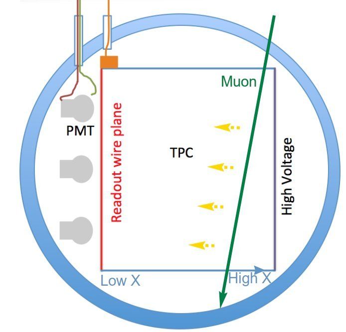
Contents

1 Introduction 1

2 Simulation of Cosmic Activity in MicroBooNE 2
 2.1 Geometry 3
 2.2 Cosmic-Ray Generators 3
 2.3 Simulated Muon Rate 4

3 Atmospheric Muon Characterisation with the Time Projection Chamber 5
 3.1 Space Charge Effect in LArTPC’s 5
 3.2 Muon Selection: Purity and Efficiency 7
 3.3 Muon Reconstruction Performance in Simulation 7
 3.4 Comparison of the Data and Predicted Rates 9
 3.5 Systematic Uncertainty Estimation 10

4 Muon Rate Measurement using the Photon Detection System 14
 4.1 Optical Reconstruction 14
 4.2 Optical Interaction Rate 14
 4.3 Systematic Uncertainty Estimation 15

5 Conclusion 17

1 Introduction

The MicroBooNE experiment is a neutrino detector located at Fermilab. Its main detector compo-
nent is a Liquid Argon Time Projection Chamber (LArTPC) placed inside a cylindrical cryostat.
Charged particles ionise the liquid argon while traversing the TPC. These ionisation electrons drift
under the influence of an electric field and are sensed by three wire planes. The collection plane
wires are vertical, while the wires on the two induction planes are offset by +60° and −60° with
respect to the vertical. MicroBooNE is further equipped with an optical system of 32 units that
provides an event trigger. Each optical unit consists of a 8-inch diameter Hamamatsu R5912-02mod
cryogenic photomultiplier tube (PMT) inside a mu-metal shield. The PMTs are positioned behind
individual tetraphenyl butadiene (TPB) coated acrylic plates to shift the VUV scintillation light
created by interactions in the cryostat. A detailed description of the MicroBooNE detector can be
found in [1].
 The MicroBooNE experiment is subject to a large atmospheric-muon flux due to its near-
surface location. The centre of the TPC is located 6 m below the surface in a concrete open pit in
the liquid argon test facility building (LArTF). The large TPC dimensions – the width ( ) of 2.6 m,
the height ( ) of 2.3 m and the length ( ) of 10.4 m – lead to a large rate of cosmic particles.

 –1–

The TPC operating voltage of −70 kV is applied to the cathode, producing an electric field
between the cathode and the anode in the -direction. Therefore, the TPC charge collection time is
approximately 2.3 ms, long enough to accumulate several atmospheric muons passing through the
TPC. The majority of recorded events will consist of cosmic-ray activity, resulting in an important
background for neutrino interaction measurements.
 In MicroBooNE, the main method we use to estimate the impact of cosmic activity on neu-
trino physics relies on data recorded when the neutrino beam is turned off. This is done in two
configurations. First, the external data stream records events that are triggered by optical signals
from cosmic activity in an identical way as the neutrino data stream. Data taken with the external
data stream is used to account for events triggered by cosmic activity when the beam was on but
no neutrino interacted. Second, an unbiased data stream records cosmic data in the usual event
format without the optical trigger requirements. This data can then be overlaid with simulated
neutrino activity. When correctly scaled to the number of protons on target, these overlay events
can be combined with events from the external data stream and compared with beam-on data.
These beam-off data streams can only be collected when the detector is operational. Even after
several years of data-taking, the amount of beam-off data in both of these configurations is limited
by operational constraints. Therefore, either for background studies before the experiment was
fully commissioned, or for increased background statistics, accurate simulation of cosmic activity
is essential.
 This work uses the unbiased data stream to validate the accuracy of simulated cosmic events.
The simulation is scaled to the data using the exposure time. The results presented guide the
simulation of cosmic activity for future near-surface experiments at Fermilab such as Mu2e, SBND,
ICARUS and the DUNE prototype detectors at CERN [2–4]. The cosmic-ray Monte Carlo (MC)
simulation and its configuration are presented in section 2.
 LArTPCs are novel and complex detectors. In section 3, the MicroBooNE TPC is used to
study the tracks created by atmospheric muons. Detector effects are discussed and we demonstrate
that these are well modelled and understood. The optical system of MicroBooNE can be used to
count muons, as is described in section 4.
 Independently of the importance for neutrino searches, the first atmospheric muon rate mea-
surement with a surface-based liquid argon detector at Fermilab is presented. In section 5, the
observed rates in the TPC and PMT systems are converted into an integrated atmospheric muon
rate at the MicroBooNE TPC and above the roof of the building. The measurements from the two
independent systems are found to agree with one another.

2 Simulation of Cosmic Activity in MicroBooNE

Cosmic rays are produced when galactic protons – or heavier elements such as helium and up to
iron – interact with the Earth’s atmosphere. These interactions lead to extensive air showers that
contain a large number of cosmic-induced particles, here referred to as primaries. The composition
and the flux of these particles depends on the location – latitude, longitude and altitude – as well as
the amount of shielding above the detector.

 –2–

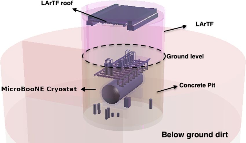
2.1 Geometry
Fermilab is located at a latitude of 41°5001500 North and a longitude of 88°1601000 West. The
MicroBooNE TPC is located inside an open concrete pit, 6 m underground and is at an elevation
of 228 m above mean sea level. The MicroBooNE simulated geometry includes the full LArTF
building, with the roof and the concrete pit as well as the detector cryostat. The platform and
electronics racks located on top of the cryostat are also included as shown in figure 1. Muons
are mainly affected by the concrete elements (density of 2.3 g/cm3 ) and the dirt surrounding the
building (density of 1.7 g/cm3 ).

Figure 1: Geometry of the simulated MicroBooNE detector and surroundings. In order to show
the details of the simulation, a transparent view of the LArTF geometry is shown.

2.2 Cosmic-Ray Generators
The cosmic-ray simulation used by MicroBooNE is CORSIKA version 7.4003 [5]. Comparisons
between this generator and CRY – another Monte-Carlo-based cosmic ray simulation library [6] –
were performed. Both generators predict similar muon rates. CORSIKA was chosen because of
the additional flexibility offered, such as the inclusion of longitudinal effects due to the movement
of the Earth in the Milky Way [7] and a modifiable incoming flux of extra-terrestrial particles.
 The production of cosmic-ray particles in the Earth’s atmosphere depends on the intensity of
nucleons per energy-per-nucleon. The energy of the nucleons is approximately independent of
whether the incident nucleons are free protons or are bound in heavier nuclei. The intensity of
cosmic nucleons can be modelled by [8]:

 nucleons
 Φ( ) = 1.8 × 104 ( [GeV]) −2.7 , (2.1)
 m2 s sr GeV
where is the energy-per-nucleon. In this work, in the default configuration, all galactic particles
are modelled as cosmic protons. Especially at higher energies, components such as helium nuclei [9]
and, in smaller fractions carbon, oxygen and even heavier nuclei contribute [10].
 An alternative CORSIKA model of the extra-terrestrial flux, the constant mass composition
(CMC) model, is used for comparison. While maintaining the same spectral index of 2.7, this
model has strong contributions from five mass groups: = 1 for protons, = 4 for helium nuclei,

 –3–

 = 14 for the CNO group, = 28 for the Mg-Si group, and = 56 for the Fe group, where is
the average mass number [11].
 Hadronic interactions in the air showers are modelled by FLUKA [12]. The default configura-
tion is summarised in table 1

Table 1: The configuration parameters used in the comparisons with measurements later in this
article. This configuration will be referred to as CORSIKA default. The magnetic components are
obtained from the latitude and longitude using NOAA [13].

 Parameter Value
 CORSIKA v7.4003
 Hadronic interaction model FLUKA 2011
 Flux constant 1.8 × 104
 Flux energy slope −2.7
 Elevation 228 m
 Magnetic field north-component 19.066 µT
 Magnetic field vertical-component 50.628 µT

2.3 Simulated Muon Rate
The simulated muon rate, [events/s/m2 ], is obtained after integrating the muon flux over the muon
energy and solid angle. This quantity is related to the often quoted integral intensity of vertical
muons [events/s/m2 /sr] using the zenith angle distribution, ( ):
 ∫ ∫
 2
 [events/s/m ] = ( ) ( ) dΩd , (2.2)
 Ω 

where it is assumed that the muon rate can be factorised in the muon energy, the azimuthal angle
and the zenith angle. In the case of azimuthal symmetry this reduces to:
 ∫ /2
 [events/s/m2 ] = 2 ( ) sin d . (2.3)
 0

Often used analytical approximations for ( ) are cos2 and exp(1 − 1/cos ) [14].
 The propagation of the primary particles produced by the cosmic-ray generator inside the
MicroBooNE environment is performed by the Geant4 program [15]. The muon trajectory is
described by a set of interaction points with corresponding energy losses. Due to the shielding
provided by the walls of, and earth surrounding, LArTF and the liquid argon inside the cryostat
surrounding the TPC, muons at the surface need a certain momentum to penetrate into the TPC.
This momentum threshold depends on the angle of the incoming muon, ranging from & 0.3 GeV/c
for vertical muons to & 1.5 GeV/c for muons with an incident angle of 75° with the zenith.
 The trajectory of the simulated muon ends when the muon leaves the environment or stops
inside the TPC. The physics processes simulated are different for + and − . Muon decay is the only
mechanism simulated for a stopped + in the TPC, leading to a Michel positron. For stopped − ,
the dominant physics process is nuclear absorption ( − + → + ), leaving no visible signature

 –4–

in the TPC. The remaining fraction of stopped − in the TPC volume decay to Michel electrons.
Overall, in simulation 11.6 ± 0.1% of the atmospheric muons entering the TPC stop in the TPC.
 The atmospheric muon rate at the Earth’s surface as predicted by different cosmic-ray sim-
ulations is given in table 2. The rate of muons entering the MicroBooNE TPC volume, pre-
dicted with the default CORSIKA configuration and obtained with the full detector simulation, is
(4388 ± 9) events/s (stat). Equivalently, this corresponds to O (10) atmospheric muons in a drift
window of 2.3 ms, stressing the importance of understanding and modelling this background in
near-surface LArTPCs.

Table 2: Surface muon rates at the geomagnetic location of Fermilab with an altitude of 228 m for
different cosmic-ray simulations. The rates are integrated over energies and angles. The quoted
errors are statistical. The predicted rate with the CMC model is significantly higher than the default
model, demonstrating the effect of the incoming flux parametrisation. The CMC model was chosen
to provide an upper limit of the expected cosmic backgrounds in the MicroBooNE experiment.

 CRY CORSIKA default CORSIKA CMC
 ± flux [events/s/m2 ] 120.0 ± 0.2 127.7 ± 0.2 160.9 ± 0.3

3 Atmospheric Muon Characterisation with the Time Projection Chamber

When a muon with an energy in the range 0.1 GeV to 100 GeV propagates through the liquid argon,
it behaves approximately as a minimum ionising particle, depositing ≈2.1 MeV/cm [8, 16] and
follows a roughly straight trajectory. Small deflections at low muon energies . 1 GeV arise from
multiple Coulomb scattering [17]. Knock-on electrons, called -rays, can have a high enough energy
to appear as small side-tracks of the muon. In liquid argon, approximately two -rays above 4 MeV
are created every meter [18, 19]. Muons decaying into a Michel electron or positron inside the TPC
create a small electromagnetic shower with a visible energy peaked at ≈20 MeV [20]. In the TPC,
the position of atmospheric muons along the drift direction is unknown, therefore, it is not possible
to distinguish a muon leaving the front or back face of the TPC from a stopping muon, unless the
Michel decay is observed. Furthermore, because scattering, ionisation, and -ray production do not
depend strongly on the muon momentum, this momentum cannot be determined for muons above
≈5 GeV.

3.1 Space Charge Effect in LArTPC’s
To correctly reconstruct muon trajectories in the TPC, a good knowledge of the magnitude and
direction of the electric field is crucial. The electric field is assumed to be uniform between the
cathode and the anode plane. However, the continuous cosmic activity in combination with the
slow drift time of the positive ions leads to a build-up of positive charge in the TPC, distorting
the electric field. The effect of this distortion on the reconstructed position of collected ionisation
electrons is referred to as the space charge effect [21]. The magnitude and the direction of this
effect depends on the position of the deposited charge. Effectively, the majority of tracks inside the
TPC have a reconstructed length that appears shorter than their simulated length. The magnitude

 –5–

(a) Wire waveform signals. The colour scale represents the amount of deposited charge.

 (b) The same event is now overlaid with the reconstructed track objects in dark red.

Figure 2: Example event containing cosmic data as recorded on the collection plane. The horizontal
axis corresponds to the wire number and the vertical axis to the charge collection time. The total
time is 3.2 ms, which includes the 2.3 ms that corresponds to one full drift width of the TPC. The
white box zooms in on a fraction of the track to highlight the level of detail in the TPC, where a
 -ray is clearly visible.

of the space charge effect is bigger for charge deposited far away from the collection planes (drift
direction) and charge deposited near the edges in the plane perpendicular on the drift direction. The
correction ranges up to O (10 cm).
 Throughout this work, two models are used and compared to take into account the space charge
effect; a simulation-based model and a data-driven one. Both models are static approximations of
the effect and ignore small time variations due to operational conditions.
 The simulation-based model makes use of a Fourier series solution with boundary conditions
to solve for the static electric field in a three-dimensional grid inside the TPC. The correction in the
reconstructed position of ionisation electrons is obtained from the electric field solution using the
Runge-Kutta-Fehlberg method (RKF45) for ray-tracing [22].
 The data-driven model uses an integrated UV laser system in combination with samples
of through-going atmospheric muons. Both the laser and atmospheric muon methods enable
MicroBooNE to further calibrate the residual space charge effects after applying the simulation-
based model [23].

 –6–

In section 3.4 both models will be compared with data and with the uncorrected simulation.
The data-driven space charge effect correction is used as the default, the difference between the
models is used to estimate a systematic uncertainty in section 3.5. Differences between data and
simulation in the field response which could lead to biases in the reconstruction efficiency for either
the track length or angles are discussed in [24, 25] and covered by the different space charge models.

3.2 Muon Selection: Purity and Efficiency
The straight muon trajectories are reconstructed as track objects using the cosmic reconstruction
configuration of the Pandora reconstruction framework [26]. An example event display, as seen
by the collection plane, before and after track reconstruction is shown in figure 2. Tracks with a
reconstructed track length longer than 25 cm are selected as muons and are used to study the purity
and efficiency. Of simulated muons that intersect the TPC, 6.8% have path lengths shorter than
25 cm. The selection purity is defined as the fraction of selected tracks for which the reconstructed
charge is dominantly deposited by the simulated muon. Additionally, the reconstructed track
needs to be uniquely associated to the simulated muon. The obtained purity for the selection is
97.71 ± 0.02% (stat).
 Of the selected tracks, 1.32 ± 0.01% (stat) are not uniquely matched to a simulated muon.
This is the case when a simulated muon is reconstructed as two separate tracks, for example, due
to a scatter or the presence of an unresponsive wire region in the detector [26]. The remaining
0.97 ± 0.01% (stat) of the selected tracks are created by cosmogenic neutrons through inelastic
scattering (in two thirds of the cases) and cosmogenic protons (in one third).
 The muon reconstruction efficiency, 97.84±0.05% (stat), is defined as the fraction of simulated
muons with a length of at least 25 cm inside the TPC that have a corresponding reconstructed track
of at least 25 cm. The inefficiency of ≈ 2% has two causes. First, ≈ 10% of the charge read-out
wires of the TPC are unresponsive [27]. A track with a significant portion of its trajectory lost
due to unresponsive wires will not be reconstructed. Second, the reconstructed track length can be
shorter than 25 cm, either because of unresponsive wires or of space-charge effects.
 The reconstruction efficiency of 97.84 ± 0.05% (stat) is in agreement with a previous data-
driven efficiency measurement using an external muon counter system that found 97.1 ± 0.1 (stat) ±
1.4 (sys)% [28].

3.3 Muon Reconstruction Performance in Simulation
The reconstructed muon-track length and angles are defined in figure 3. Before the in-TPC segment
of the simulated muon trajectory is compared with the reconstructed track, a data-driven space
charge effect correction is applied on the trajectory [23].
 The muon reconstruction resolution is determined by comparing the reconstructed quantities
with the underlying simulated information for the different muon parameters – length and angles –
using reconstructed tracks that meet the selection criterion.
 In each bin of a simulated variable (length or angles) we find the distribution of the difference
between the reconstructed and simulated variable, as illustrated in figure 4. The median is used to
estimate the central value. The ranges between the median 16th and 84th percentiles respectively
are used to estimate the 68% confidence interval for that bin. The resolution obtained is presented
in the panels of figure 5.

 –7–

Y

 Y

 A X

 Azimuth
 Wire planes

 X Z
 B Zenith
 Z

Figure 3: Schematic representation of a muon (green) crossing the MicroBooNE TPC. The muon
enters the TPC at point and exits the TPC, or stops inside it, at point . The track length, azimuth
and zenith angles are obtained from the segment . The left diagram illustrates the position of a
few wires of each of the three planes (grey) and the direction of the drifting electrons (orange).

 Simulated track length [125cm, 150cm] MicroBooNE Simulation
 Median (-2.3cm)
 0.20 5th percentile (-16.4cm)
 95th percentile (-6.3cm)
 track length
 Area Normalised

 0.15 1 CI, width: 6.0cm

 0.10

 0.05

 0.00
 40 30 20 10 0 10 20
 Reconstructed track length - simulated track length [cm]

Figure 4: Example of how the resolution is quantified, here shown for the track length, for tracks
with a simulated length between 125 cm and 150 cm. In blue, the histogram shows the difference
between the simulated and reconstructed length. The median is given in red, the offset between the
median and 0 is referred to as the bias. The resolution defined as half the width of the green shaded
area, covering a symmetric 68.3% interval around the median. The 5th (orange) and 95th (purple)
percentiles define a region that includes 90% of the tracks. The tail towards shorter reconstructed
tracks is explained by tracks entering or exiting through unresponsive wire regions.

 The median track length shown in the left panel of figure 5, indicates that reconstructed muon
segments are slightly shorter than the true length. The bias ranges from 0.3 cm to 2.4 cm, depending
on the true length. The 68.3% confidence interval presents a tail towards shorter tracks, as can
also be seen from the specific example in figure 4. The resolution, defined as half the width of the
68.3% interval, varies from ≈1.5 cm, for short and vertically crossing tracks and up to ≈4.0 cm for
the longest tracks.
 The middle and right panels of figure 5 show the zenith and azimuth angle resolution for the
muon segments. The bias of the median reconstructed angle is less than 0.1° in both cases. The
resolution of the zenith angle is approximately 0.2°, except for the first bin which has a tail towards

 –8–

MicroBooNE Simulation
 20 3 3
 15 median + 68% CI median + 68% CI median + 68% CI
 2 2 103
track length angle [cm]

 azimuth angle [degree]
 zenith angle [degree]
 10
 1 1

 Tracks per bin
 5
 102
 0 0 0
 5 -1 -1
 10 101
 15 -2 -2
 20 -3 -3 100
 100 200 300 400 500 0 /8 /4 3 /8 /2 /2 0 /2
 Simulated length in TPC [cm] Simulated trajectory zenith angle Simulated azimuth angle

Figure 5: Reconstruction resolution for the track length (left), zenith angle (middle) and azimuthal
angle (right). The vertical axis shows the difference between the reconstructed and the simulated
quantity. The space-charge model is applied to the simulation before comparison to data. The
colour scale of the 2D histograms is logarithmic. In black, the median of each bin with the 68.3%
confidence interval are given.

larger zenith angles, corresponding to tracks parallel to the collection wire plane and creating a
single hit which is harder to reconstruct. The resolution of the azimuthal angle varies between 0.2°
and 0.5°, depending on the track length and its alignment with the charge-collecting wires.

3.4 Comparison of the Data and Predicted Rates

In figures 6 to 8, events from the unbiased data stream are compared with simulated cosmic events.
The data sample was collected between February and May 2016 and comprises 25k events, each
consisting of a TPC readout window of 3.2 ms. The sample has no overlap with accelerator neutrino
triggers.
 As introduced in section 3.1, two variants of the space charge effect model are used in the
simulated samples. A data-driven approach is used as the nominal model, indicated as data-driven
space charge and shown in green. The theoretically derived correction is referred to as simulated
space charge and shown in orange. A case where no space charge effect is taken into account,
demonstrating the magnitude and shape of its impact, is also included and shown in red. The
data-driven space charge correction is taken as the default (central value) and the corresponding
ratio of data to simulation, integrated over the muon momentum and direction, is 1.014 ± 0.004
(stat). The systematic uncertainties will be discussed in section 3.5.
 The track length distribution in figure 6 is peaked at ≈2.3 m, corresponding to the full height of
the TPC, where top-bottom through-going muons pile up. A sharp turn on of the peak can be seen
when no space charge is simulated (red). When the space charge effect is taken into account, the
peak gets smeared out towards shorter reconstructed track lengths. The data in this region is situated
between the two different space charge models, indicating that the sample with theory-based space
charge correction (green) slightly exaggerates the effect and the sample with the data-driven model
(orange) slightly underestimates it.
 The comparison of the cosine of the reconstructed zenith angle in data and simulation is shown
in figure 7. The zenith angle has an intrinsic energy dependence due to the centre of the TPC being

 –9–

MicroBooNE
 CORSIKA, simulated space charge Tracks > 25cm
 CORSIKA, data-driven space charge Data/MC ratio: 1.01
 15000 CORSIKA, without space charge
 Tracks per bin
 Cosmic Data
 10000

 5000

 0
 1.5
 Data/MC

 1.0
 0.5
 50 100 150 200 250 300 350
 Track length [cm]

Figure 6: Comparison of the reconstructed track length in data (blue crosses) and CORSIKA Monte
Carlo simulation, with data-driven (green), with theory-based (orange), and with no (red) space
charge effect included. The bin width on the horizontal axis is 5 cm. The bottom panel shows the
ratio of data to simulation in green (Data/MC) for the sample with data-driven space charge. The
overall ratio is 1.014 ± 0.004 (stat).

located 6 m underground. Muons at larger zenith angles, being more horizontal, traverse a larger
distance in both the atmosphere and the dirt surrounding LArTF before entering the cryostat. This
is studied in the bottom panel of figure 7. The bulk of the muons entering the TPC have an energy
below 3 GeV. For muons entering more horizontally, the median energy increases up to 15 GeV.
Due to the limited extent of the simulation, zenith angles above 75° are not well covered and the
simulation underpredicts the horizontal muon flux.
 The zenith angle dependence is compared to two analytical models [14]. In the specific case of
these two analytical models, the models are normalised to the data to compare the shapes, as shown
by the shaded bands in the top and middle panel of figure 7. These models do not account for the
detector acceptance and shielding; nevertheless, their shape follows the simulation and data.
 The generation of atmospheric muons is isotropic in the azimuthal space, but the acceptance
of the cuboid shape of the MicroBooNE TPC affects the observed distribution, as can be seen in
figure 8. Small features in the ratio of data to simulation at 0° and 180° are caused by tracks parallel to
the wire planes, where the drifted charge over the whole track length arrives coincidentally, making
both the reconstruction and modelling challenging. Removal of coherent noise, in particular, affects
the reconstruction for this topology [27].

3.5 Systematic Uncertainty Estimation
Using the central value simulation, as introduced in section 2 and including a data-driven space
charge effect correction, the ratio of data to simulation is 1.014 ± 0.004 (stat). Four sources of
systematic uncertainties that impact the ratio are evaluated:

 1. Incomplete angular coverage. Limitations of the simulation show up as discrepancies between
 the data and simulation in some regions of the distributions in figures 7 and 8. The difference

 – 10 –

MicroBooNE
 CORSIKA, simulated space charge I( ) = I0 cos2
 25000 CORSIKA, data-driven space charge I( ) = I0 exp(1 1/cos )
 CORSIKA, without space charge Cosmic Data
 Tracks per bin 20000
 Tracks > 25cm
 15000 Data/MC ratio: 1.01

 10000

 5000

 0
 1.5
 Data/MC

 1.0
 0.5
 20
 True muon energy [GeV]

 Median and 68% CI
 15
 10
 5
 0
 0.0 0.2 0.4 0.6 0.8 1.0
 Cosine of reconstructed track zenith angle

Figure 7: Comparison of the cosine of the reconstructed zenith angle in data (blue crosses) and
CORSIKA Monte Carlo simulation, with data-driven (green), with theory-based (orange), and with
no (red) space charge effect included. The middle panel shows the ratio of data to simulation for
the sample with data-driven space charge. The shaded bands (grey and red) are area normalised
analytical models of the zenith dependence of atmospheric muons. In the middle panel, those models
are compared with the data-driven space charge sample. The 2D histogram in the bottom panel
shows the true muon energy for the data-driven space charge sample. For each bin, the horizontal
black line indicates the median true energy and the bars correspond to the 68.3% interval. Although
the full phase space of downward-going tracks is given, the simulation significantly undercovers
the horizontally oriented tracks – 75° and higher – due to the finite extent of the simulation. See
section 3.5 for a further discussion.

 between the data and the simulation calculated with and without these regions is taken as a
 systematic uncertainty.

 • Zenith angle. For zenith angles between 3° and 70°, the ratio is 1.010.
 • Azimuth angle. Without a region of 2° on either side of the azimuthal 0° and 180° –
 where the tracks are parallel to the collection plane – the ratio is 1.008.

 2. Length criterion. An increased muon purity can be achieved by increasing the track length
 criterion above 25 cm. In the top panel of figure 9, the purity is evaluated for minimum

 – 11 –

MicroBooNE
 15000 CORSIKA, simulated space charge Tracks > 25cm
 CORSIKA, data-driven space charge Data/MC ratio: 1.01
 12500 CORSIKA, without space charge
 Tracks per bin
 10000 Cosmic Data
 7500
 5000
 2500
 0
 1.5
 Data/MC

 1.0
 0.5
 3 /4 /2 /4 0 /4 /2 3 /4
 Azimuthal angle of reconstructed track [rad]

Figure 8: Comparison of the reconstructed track azimuth angle in data (blue crosses) and CORSIKA
Monte Carlo, with data-driven (green), with theory-based (orange), and with no (red) space charge
effect included. The bottom panel shows the ratio of data to simulation for the sample with
data-driven space charge. The bin width on the horizontal axis is 8◦

 lengths ranging from 5 cm to 175 cm. In the bottom panel, the effect on the ratio of data to
 simulation is shown. For the simulated sample with the data-driven space charge effect, the
 ratio changes from 1.014 to 1.000 when changing the track length requirement from 25 cm
 to 175 cm.

 3. Space charge effect. As demonstrated in figure 6, the space-charge effect shortens the
 reconstructed length of tracks. In the bottom panel of figure 9, the ratio of data to simulation
 is evaluated for different space charge models. The difference between the theory and data-
 driven model at a length criterion of 25 cm is 0.7%.

 4. LArTF building geometry. The details of the geometry used for the simulations, such as the
 concrete walls or the roof can impact the simulated atmospheric muon rate in the TPC. The
 potential effect is conservatively estimated by varying the concrete density of the walls and
 roof by +30% (increased LArTF building) and −30% (reduced LArTF building), leading to
 an increase of 2.7% and decrease of 1.5% in the ratio, respectively.

The different sources of systematic uncertainty are listed in table 3 and are combined in quadrature,
resulting in a ratio of data to simulation of
 +0.028 (sys)
 1.014 ± 0.004 (stat) −0.022

The size of the systematic uncertainty is indicated by the green shaded area in the bottom panel
of figure 9 and covers all the values of the ratio obtained from combining different samples and
different length criteria.

 – 12 –

Table 3: Contribution of the different systematic uncertainties on the TPC muon rate measurement.

 Systematic variation Uncertainty
 Zenith angle phase space −0.4%
 Azimuth angle phase space −0.6%
 Length criterion −1.4%
 Space charge model +0.7%
 Increased LArTF shielding +2.7%
 Decreased LArTF shielding −1.5%
 Total −2.2% / +2.8%

 MicroBooNE Simulation
 1.000
 0.975
 Muon selection purity

 0.950
 0.925
 0.900
 0.875
 0.850 CORSIKA, simulated space charge CORSIKA, reduced LArTF building
 CORSIKA, data-driven space charge CORSIKA, increased LArTF building
 0.825 CORSIKA, without space charge 25cm cut
 0.800
 MicroBooNE
 1.08 CORSIKA, simulated space charge CORSIKA, reduced LArTF building
 Ratio of data to simulation

 CORSIKA, data-driven space charge CORSIKA, increased LArTF building
 1.06 CORSIKA, without space charge 25cm cut
 1.04
 1.02
 1.00
 0.98
 0 20 40 60 80 100 120 140 160
 Length cut [cm]

Figure 9: Top: Impact of different length criteria on the muon selection purity. Bottom: The ratio
of the data to simulation rates as a function of the minimum track length requirement, for different
simulated samples. In orange, the purity (top) and ratio (bottom) are given using the sample with
data-driven space charge effect included. In blue, a sample with the theory-based space charge
simulation is shown. In green, a sample without simulated space charge is shown. The purple and
red curves correspond to samples with data-driven space charge effect where the concrete density
of the LArTF building is varied with ±30%. The green band represents the combined systematic
uncertainty as obtained in table 3. The grey line shows the 25 cm requirement used in this work.

 – 13 –

4 Muon Rate Measurement using the Photon Detection System

The muon rate is independently measured using MicroBooNE’s optical system, consisting of 32 8-
inch PMTs. The rate of optically reconstructed signals can be related to the atmospheric muon-rate,
validating the TPC-based measurement.

4.1 Optical Reconstruction
The optical reconstruction builds flashes from the PMT waveforms. Flashes represent coincidental
optical activity across several PMTs, usually caused by a particle interaction in the TPC. An
example is illustrated in figure 10. A flash object is created when at least two PMTs detect a
signal corresponding to at least 8 photoelectrons (PEs), each in a coincidence interval of 94 ns.
The flash object contains the light of the different PMTs that crossed the 8 PE threshold, integrated
during 625 ns. This window covers the 6 ns prompt (and a fraction of the 1.5 µs slow) scintillation
component of liquid argon. A veto window of 8 µs is applied after the creation of a flash to avoid
the creation of spurious flashes due to the tail of the slow scintillation light component.

 Run 5075, Subrun 3, Event 185 MicroBooNE Data
 100
PMT postion y [cm]

 50
 0
 50
 100
 0 200 400 600 800 1000
 PMT postion z [cm]

Figure 10: Example of a flash, consisting of multiple PMT signals combined. The orange colour
scale is logarithmic and represents the intensity of the light, arriving in each PMT, integrated over
625 ns. The blue cross indicates the location of the centre of the flash. The 32 PMTs are organised
in five rosettes, located behind the wires in the -plane.

4.2 Optical Interaction Rate
Purity In simulation, 94.1 ± 0.1% (stat) of the reconstructed flashes are matched to simulated
muons. The majority of the remaining fraction originated from light induced by inelastic neutron
scattering. The 94.1 ± 0.1% (stat) can be divided into muons entering the TPC (81.6 ± 0.1%), and
flashes caused by muons that enter the cylindrical cryostat but do not pass through the cuboid TPC
volume 12.6 ± 0.1% (stat).

Reconstruction efficiency Of the simulated atmospheric muons entering the TPC, 81.3 ± 0.3%
(stat) lead to a reconstructed flash. The 8 µs veto window causes an additional loss of 4.8% due to
dead time. A further inefficiency is due to geometrical effects, illustrated in figure 11, where the
flash efficiency is reduced for simulated muons at high , far from the PMTs. A similar, although
less pronounced, effect is found at the TPC edges in the -plane and is accounted for as a systematic
uncertainty in section 4.3.

 – 14 –

Flashes of simulated muons MicroBooNE Simulation 103
 2500
 All muons
 7000 Muons without flash
 6000 Muons with flash 2000

 Flash intensity [PE]
 5000 102

 Entries per bin

 Entries per bin
 1500
 4000
 3000 1000
 101
 2000
 500
 1000
 0 100
 0 50 100 150 200 250 0 50 100 150 200 250
 Muon average x in TPC [cm] Muon average x in TPC [cm]

Figure 11: (Left) Schematic side view of the MicroBooNE cryostat, showing a muon crossing
near the cathode (high ). (Middle) Average position of the crossing muon trajectory inside the
active TPC volume. The simulated muons (green) are divided in those that have a corresponding
reconstructed flash 81.6±0.1% (blue), and those that do not (orange). The central peak corresponds
to the average location of anode-cathode crossing muons. Note the sharp decline for tracks situated
within half a meter from the cathode plane. (Right) The flash intensity versus the average muon
distance from the wire planes. The logarithmic colour scale represents the number of flashes per
bin. Far from the anode, the flash intensity is strongly reduced.

 After correcting for the dead time introduced by the veto window, the flash rate in simulation
is (4.642 ± 0.011) kHz (stat). Using the same data sample as in section 3.4, a flash rate of
(4.593 ± 0.007) kHz (stat) is obtained, after the dead-time correction. These results do not include
systematic uncertainties, which are described in the next section.

4.3 Systematic Uncertainty Estimation
The sources of systematic error can be divided into light modelling systematic uncertainties and the
uncertainty from the LArTF geometry simulation and are listed below:

 1. Flash photoelectron threshold. Flashes are created with a minimum of optical-activity of
 34 PE. This threshold can be increased to evaluate the sensitivity of the ratio between data
 and simulation due to the very dimmest flashes. After doubling the threshold to 68 PE in
 both data and simulation, this ratio changes from 0.990 to 0.992, resulting in a systematic
 uncertainty of 0.2%. The effect of this change is shown in the right panel of figure 12.

 2. Light yield variations. The impact of a difference in absolute light yield between simulation
 and data is evaluated by varying the total flash intensity by ±30% in simulation. The change
 in light yield manifests itself as a different threshold in data and simulation, as illustrated in
 the right panel of figure 12. The decreased scintillation light production leads to a data to
 simulation ratio of 1.006, the increased light yield leads to a ratio of 0.974. Therefore this
 uncertainty is symmetric and affects the result by 1.6%.

 3. Out-of-TPC light modelling. As discussed in section 4.2, a fraction of the flashes are caused
 by muons crossing the cryostat without entering the TPC. Their impact on the ratio can
 be studied by restricting the measurement to flashes which are centred inside a constrained

 – 15 –

MicroBooNE MicroBooNE
 105
 CORSIKA
 7000 Cosmic data (Run 1)
 Flashes per bin

 Flashes per bin
 104 6000

 5000
 CORSIKA
 Cosmic data (Run 1)
 103 4000
 0 1000 2000 3000 4000 44 68 100 140 180
 Flash Intensity [PE] Flash Intensity [PE]

Figure 12: Comparison of the flash intensity, expressed as a number of photoelectrons (PE), in
simulation and data. The right panel zooms in for low-intensity flashes. The two vertical grey lines
correspond to the investigation of systematic uncertainties introduced by the increased threshold
(68 PE) and the ±30% variation in light yield (44.2 PE). The shaded area (CORSIKA Simulation)
and vertical crosses (Cosmic Data) represent the statistical variation.

 region in the -plane (green shaded area in figure 13). Excluding flashes that are centred
 less then 1 m away from the edges in the -direction and less than 30 cm from the top in the
 vertical direction, the contribution of flashes caused by muons inside the cryostat without
 entering the TPC decreases from 12.6% to 6.2%. The ratio of data to simulation changes
 from 0.990 to 0.992. The systematic uncertainty is taken to be twice the difference in the
 ratio to account for the 6.2% remaining contribution of flashes caused by activity outside of
 the TPC.

 z center of the flash - MicroBooNE y center of the flash - MicroBooNE
 CORSIKA (4.5 kHz) CORSIKA (4.5 kHz)
 Cosmic data (4.4 kHz) Cosmic data (4.4 kHz)
 40000 In-TPC ±
 Out-TPC ±
Flashes per bin

 Flashes per bin

 20000 30000 Other type
 20000
 10000
 10000
 0 0
 1.5 1.5
 Data/MC

 Data/MC

 1.0 1.0
 0.5 0.5
 0 200 400 600 800 1000 60 40 20 0 20 40 60
 Flash z [cm] Flash y [cm]

Figure 13: Position of the centre of the flash in the (left) and (right) directions. The flashes
from muons entering the TPC are shown in blue, from muons entering the cryostat but not the TPC
in orange, and a small contribution of non-muon particles is shown in green. The shaded green
indicates the restricted area where the contribution of out-TPC muons is reduced. The five bumps
structure is explained by the position of the PMTs as shown in figure 10.

 4. LArTF geometry modelling To account for potential mismodeling of the building geometry,

 – 16 –

two samples, one with increased and one with decreased concrete density, are used to estimate
 the effect on the flash rate. Increasing the concrete density by 30% leads to a reduction in
 flash-rate of 2.7%, while decreasing the density with 30% increases the flash-rate by 2.3%.

 The different sources of systematic uncertainty are listed in table 4, the total systematic error
is obtained by adding the different contributions in quadrature. The ratio of data to simulation is:
 +0.032 (sys).
 0.990 ± 0.003 (stat) −0.028

 Table 4: Systematic uncertainties on the PMT muon rate measurement.

 Systematic variation Uncertainty
 Flash photoelectron threshold +0.2%
 Light yield variations ±1.6%
 Out-of-TPC light modelling +0.4%
 Increased LArTF shielding +2.7%
 Decreased LArTF shielding −2.3%
 Total −2.8% / +3.2%

5 Conclusion

In sections 3 and 4, we present ratios between the muon rate in data and simulation. These ratios
can be converted into the muon flux per area at the position of the detector. To obtain this rate, the
simulated rate is scaled by the ratio between the data and simulated rate. This rate does not depend
on the systematic uncertainty introduced by the LArTF geometry since the variation in simulated
shielding cancels out in the observed ratio. The atmospheric muon rate obtained independently
with the TPC and the PMTs is quoted with systematic uncertainty in the first column of table 5.
Excluding the systematic uncertainty related to the LArTF geometry, the two measurements and their
systematic uncertainties are uncorrelated. All rates are in agreement within errors. No systematic
uncertainties due to the choice of CORSIKA configuration, as was introduced in section 2.2, is
included in these results.
 Relying on the simulation of the LArTF building geometry, the measured ratios are extrapolated
to the muon rate at the Earth’s surface, which is useful for near-surface experiments located at
Fermilab. The obtained atmospheric muon flux is compared with the CORSIKA rates in the last
column of table 5. In this case, the dominant systematic uncertainty originates from the LArTF
building geometry modelling and is strongly correlated between the two measurements. These
measurements include muons with a momentum & 0.3 GeV/c (see section 2.3), but the bulk of the
detected muons are in the 1 GeV/c to 3 GeV/c momentum range, as can be seen in the bottom panel
of figure 7.
 The integrated muon flux obtained with the MicroBooNE detector is compared with other
measurements in figure 14. The results presented are in agreement with both the CORSIKA

 – 17 –

prediction of (127.7 ± 0.2) events/s/m2 and previous measurements [29–31]. Because of the
choice to integrate over the angular and muon momentum space, the result can be compared with
differential measurements using equation (2.2).

 The data used in this works spans a period of four months (February to May 2016), during which
no significant evidence of seasonal fluctuations was observed. The measured tracks are dominated
by low-energetic muons due to the lack of shielding. Furthermore, the detector technology is unable
to discriminate tracks based on the muon momentum. In these conditions, any seasonal effects are
expected to be challenging to detect at MicroBooNE [32].

Table 5: Summary of the atmospheric muon rates in simulation and data, at the TPC and extrapolated
to LArTF building roof level. The simulation rates using CORSIKA is presented, along with the
measured TPC and PMT data rates, as obtained in sections 3 and 4 respectively.

 Rate at TPC (events/s/m2 ) Rate above roof (events/s/m2 )
 Simulation CORSIKA default 111.6 ± 0.3 127.7 ± 0.2

 TPC +0.8 (sys)
 113.2 ± 0.5 (stat) −1.8 +3.6 (sys)
 129.5 ± 0.5 (stat) −2.8
 Data
 PMT +1.8 (sys)
 110.4 ± 0.4 (stat) −2.0 +4.1 (sys)
 126.5 ± 0.4 (stat) −3.5

 Fermilab 226m MicroBooNE Data
 150
 Muon flux [events / m2 / s]

 140

 130
 CORSIKA 127.7±0.2(stat.)
 120 TPC 129.5±0.5(stat.)+3.6
 2.8 (syst.)
 PMT 126.5±0.4(stat.)+4.0
 3.5(syst.)
 Mitrica B et al 2011 Nucl. Instrum. Meth. A 654 176 183
 110 D I Stanca et al 2013 J. Phys.: Conf. Ser. 409 012136
 0 200 400 600 800 1000
 Elevation [m]

Figure 14: Comparison of the integrated muon flux measurement from this work (coloured data
points) with previous measurements [30, 31] (black data points), for different elevations. The vertical
grey line indicates the elevation of Fermilab. The TPC (blue) and PMT (orange) measurements are
compared with the CORSIKA prediction (green). The vertical width of the data points represents
the statistical error, and the error bars represent the combined statistical and systematic errors added
in quadrature. The blue and orange points are horizontally offset from the grey line for visual clarity.

 – 18 –

Acknowledgments

This document is prepared by the MicroBooNE collaboration using the resources of the Fermi
National Accelerator Laboratory (Fermilab), a U.S. Department of Energy, Office of Science, HEP
User Facility. Fermilab is managed by Fermi Research Alliance, LLC (FRA), acting under Contract
No. DE-AC02-07CH11359. MicroBooNE is supported by the following: the U.S. Department of
Energy, Office of Science, Offices of High Energy Physics and Nuclear Physics; the U.S. National
Science Foundation; the Swiss National Science Foundation; the Science and Technology Facilities
Council of the United Kingdom; and The Royal Society (United Kingdom). This research is further
supported by the U.S. Department of Energy, Office of Science, Office of High Energy Physics,
under the Award Number DE-SC0007881. Additional support was received from Oxford University
Press and Jesus College Oxford.

References
 [1] MicroBooNE collaboration, Design and construction of the MicroBooNE detector, JINST 12 (2017)
 P02017 [1612.05824].
 [2] Mu2e collaboration, The Mu2e Experiment, Front. in Phys. 7 (2019) 1 [1901.11099].
 [3] P. A. Machado, O. Palamara and D. W. Schmitz, The short-baseline neutrino program at Fermilab,
 Annu. Rev. Nucl. Part. Sci. 69 (2019) 363 [1903.04608].
 [4] DUNE collaboration, Deep underground neutrino experiment (DUNE), far detector technical design
 report, volume I introduction to DUNE, JINST 15 (2020) T08008 [2002.02967].
 [5] D. Heck, J. Knapp, J. Capdevielle, G. Schatz and T. Thouw, CORSIKA: a Monte Carlo code to
 simulate extensive air showers. KIT, 1998, 10.5445/IR/270043064.
 [6] C. Hagmann, D. Lange and D. Wright, Cosmic-ray shower generator (CRY) for Monte Carlo
 transport codes, IEEE Nucl. Sci. Symp. Conf. Rec. 2 (2007) 1143 .
 [7] A. H. Compton and I. A. Getting, An apparent effect of galactic rotation on the intensity of cosmic
 rays, Phys. Rev. 47 (1935) 817.
 [8] P.A. Zyla et al. (Particle Data Group), Review of Particle Physics, Prog. Theor. Exp. Phys. 2020
 (2020) 083C01.
 [9] PAMELA collaboration, Measurements of cosmic-ray proton and helium spectra, Science 332 (2011)
 69 [1103.4055].
[10] D. Maurin, F. Melot and R. Taillet, A database of charged cosmic rays, A&A 569 (2014) A32
 [1302.5525].
[11] C. Forti, H. Bilokon, B. d’Ettorre Piazzoli, T. K. Gaisser, L. Satta and T. Stanev, Simulation of
 atmospheric cascades and deep-underground muons, Phys. Rev. D 42 (1990) 3668.
[12] T. Böhlen, F. Cerutti, M. Chin, A. Fassò, A. Ferrari, P. Ortega et al., The FLUKA code: Developments
 and challenges for high energy and medical applications, Nuclear Data Sheets 120 (2014) 211 .
[13] Earth’s magnetic field calculator, National Oceanic and Atmospheric Administration (2020)
 www.ngdc.noaa.gov/geomag/calculators/magcalc.shtml.
[14] P. Grieder, Cosmic rays at earth: Researcher’s reference, manual and data book. Elsevier, 2001.
[15] GEANT4 collaboration, GEANT4: A Simulation toolkit, Nucl. Instrum. Meth. A506 (2003) 250.

 – 19 –

[16] MicroBooNE collaboration, Calibration of the charge and energy loss per unit length of the
 MicroBooNE liquid argon time projection chamber using muons and protons, JINST 15 (2020)
 P03022 [1907.11736].
[17] MicroBooNE collaboration, Determination of muon momentum in the MicroBooNE LArTPC using
 an improved model of multiple Coulomb scattering, JINST 12 (2017) P10010 [1703.06187].
[18] Icarus collaboration, Determination of through-going tracks’ direction by means of delta-rays in the
 ICARUS liquid argon time projection chamber, Nucl. Instrum. Meth. A 449 (2000) 42.
[19] K. Ingles, T. Junk and A. Marchionni, Muon energy loss in liquid argon, in Fermilab SIST/GEM
 Presentations, 2017, https://indico.fnal.gov/event/14933/contributions/28526/.
[20] MicroBooNE collaboration, Michel electron reconstruction using cosmic-ray data from the
 MicroBooNE LArTPC, JINST 12 (2017) P09014 [1704.02927].
[21] MicroBooNE collaboration, A method to determine the electric field of liquid argon time projection
 chambers using a UV laser system and its application in MicroBooNE, JINST 15 (2020) P07010
 [1910.01430].
[22] M. Mooney, The MicroBooNE experiment and the impact of space charge effects, in APS DPF
 proceedings, 11, 2015, 1511.01563.
[23] MicroBooNE collaboration, Measurement of space charge effects in the MicroBooNE LArTPC using
 cosmic muons, JINST 15 (2020) P12037 [2088.09765].
[24] MicroBooNE collaboration, Ionization electron signal processing in single phase LArTPCs. Part I.
 Algorithm Description and quantitative evaluation with MicroBooNE simulation, JINST 13 (2018)
 P07006 [1802.08709].
[25] MicroBooNE collaboration, Ionization electron signal processing in single phase LArTPCs. Part II.
 Data/simulation comparison and performance in MicroBooNE, JINST 13 (2018) P07007
 [1804.02583].
[26] MicroBooNE collaboration, The pandora multi-algorithm approach to automated pattern
 recognition of cosmic-ray muon and neutrino events in the MicroBooNE detector, Eur. Phys. J. C 78
 (2018) 82 [1708.03135].
[27] MicroBooNE collaboration, Noise characterization and filtering in the MicroBooNE liquid argon
 TPC, JINST 12 (2017) P08003 [1705.07341].
[28] MicroBooNE collaboration, Measurement of cosmic-ray reconstruction efficiencies in the
 MicroBooNE LArTPC using a small external cosmic-ray counter, JINST 12 (2017) P12030
 [1707.09903].
[29] J. Kremer, M. Boezio, M. L. Ambriola, G. Barbiellini, S. Bartalucci, R. Bellotti et al., Measurements
 of ground-level muons at two geomagnetic locations, Phys. Rev. Lett. 83 (1999) 4241.
[30] B. Mitrica, R. Margineanu, S. Stoica, M. Petcu, I. Brancus, A. Jipa et al., A mobile detector for
 measurements of the atmospheric muon flux in underground sites, Nucl. Intrum. Meth. A 654 (2011)
 176 [1104.2157].
[31] D. Stanca, B. Mitrica, M. Petcu, I. M. Brancus, A. Jipa, A. Haungs et al., Measurements of the
 atmospheric muon flux using a mobile detector based on plastic scintillators read-out by optical fibers
 and PMTs, J. Phys. Conf. Ser 409 (2013) 012136.
[32] S. Cecchini and M. Spurio, Atmospheric muons: experimental aspects, Geosci. Instrum. Method.
 Data Syst. 1 (2012) 185 [1208.1171].

 – 20 –