A Novel Method for Identifying a Parsimonious and Accurate Predictive Model for Multiple Clinical Outcomes
←
→
Page content transcription
If your browser does not render page correctly, please read the page content below
A Novel Method for Identifying a Parsimonious and
Accurate Predictive Model for Multiple Clinical Outcomes
Ledif Grisell Diaz-Ramirez ( grisell.diaz-ramirez@ucsf.edu )
University of California San Francisco https://orcid.org/0000-0003-1621-9309
Sei J. Lee
University of California San Francisco
Alexander K. Smith
University of California San Francisco
Siqi Gan
University of California San Francisco
Walter John Boscardin
University of California San Francisco
Research article
Keywords: backward elimination, Bayesian Information Criterion, prognostic models, survival analysis, variable
selection
DOI: https://doi.org/10.21203/rs.2.20249/v2
License: This work is licensed under a Creative Commons Attribution 4.0 International License. Read Full
License
Page 1/28Abstract
Background: Most methods for developing clinical prognostic models focus on identifying parsimonious and accurate
models to predict a single outcome; however, patients and providers often want to predict multiple outcomes
simultaneously. For example, older adults are often interested in predicting nursing home admission as well as
mortality. We propose and evaluate a novel predictor selection method for multiple outcomes.
Methods: Our proposed method selected the best subset of common predictors based on the minimum average
normalized Bayesian Information Criterion (BIC) across outcomes: the Best Average BIC (baBIC) model. We compared
the predictive accuracy (Harrell’s C-statistic) and parsimony (number of predictors) of the baBIC model with a subset
of common predictors obtained from the union of optimal models for each outcome (Union model). We used example
data from the Health and Retirement Study (HRS) to demonstrate our method and conducted a simulation study to
investigate performance considering correlated and uncorrelated outcomes.
Results: In the example data, the average Harrell’s C-statistics across outcomes of the baBIC and Union models were
comparable (0.657 vs. 0.662 respectively). Despite the similar discrimination, the baBIC model was more
parsimonious than the Union model (15 vs. 23 predictors respectively). Likewise, in two simulation scenarios with
correlated and uncorrelated outcomes, the mean C-statistic across outcomes of the baBIC and Union models were
very similar, and the baBIC model had on average fewer predictors. In the simulations, the baBIC method performed
well by identifying the correct predictors most of the time and excluding the incorrect predictors in the majority of the
simulations.
Conclusions: Our method identi ed a common subset of variables to predict multiple clinical outcomes with superior
parsimony and comparable accuracy to current methods.
Background
One of the rst steps in building a regression model is selecting a subset of predictors from a pool of many available
predictors. Clinicians and researchers alike desire a model that explains the data in the simplest way—namely, a
parsimonious model—with appropriate predictive accuracy. Parsimonious models offer the potential to save the time
it takes to gather unnecessary predictors, and expense, either in visit time or in money.
Most current model development methods focus on accurate and parsimonious prediction of single outcomes.
Popular methodologies that are easy to use and interpret include stepwise methods like backward elimination or
criterion-based selection like the Akaike Information Criterion (AIC) (1) or the Bayesian Information Criterion (BIC) (2).
However, obtaining the most parsimonious and accurate model is more complex for the simultaneous prediction of
multiple outcomes, a common scenario in clinical settings.
Several studies have demonstrated that older adults care not only about mortality, but also about their quality of life,
speci cally their ability to function independently (3, 4). In the realm of anticoagulation for atrial brillation, for
example, clinicians may want to simultaneously predict risk of stroke and risk of a major gastrointestinal bleed (5, 6).
In primary care, clinicians may want to balance risk of microvascular complications from diabetes against the risks of
hypoglycemia and falls (7, 8). Yet, there is limited research on how best to develop clinical prognostic models that
predict multiple outcomes simultaneously with accuracy and parsimony.
Much of the research on variable selection for multiple outcomes has been done in the high-dimensional multivariate
regression setting, where the number of predictors and outcomes outweighs the number of observations. Under this
Page 2/28setting, the implementation of shrinkage or regularization methods is common (9-11). Other authors have addressed
variable selection for multivariate modelling using a Bayesian framework (12-14). However, in clinical settings, where
the sample size is frequently large relative to the number of predictors and outcomes, a simpler and easy-to-
implement procedure that does not require complex software solutions could be of great utility.
An obvious approach (which we label Individual Outcome method) to address the multiple outcomes problem is to
simply select a different subset of variables to predict each of the outcomes using selection methods for single
outcomes. Although straightforward, this method could be time-consuming, expensive (due to the cost of acquiring
multiple predictors), and potentially lead to over tting and high variability (9, 15).
A slight modi cation to this approach is the Union method. In this method, we take the separate models from the
Individual Outcome method, and then force the union of the predictors from each model into the predictor set for each
outcome. The online compendium of prognostic indices “ePrognosis” —freely available at ePrognosis.org (16, 17)—
receives over 3,000 users per week, and the most-used index is a Union model: the Combined Lee Schonberg Index,
created from union of predictors from the Lee Index (18, 19) and the Schonberg index (20, 21). Like the Individual
Outcome method, the Union method has the advantage of being a simple approach, and, additionally, it allows
patients and clinicians to focus on a common subset of variables that can accurately predict their outcomes of
interest simultaneously. Nevertheless, the Union model could lack parsimony as it includes all variables that predict all
outcomes well, including those that are only important for some of the outcomes.
In this paper, we propose and evaluate a novel method for predictor selection in prognostic models of multiple clinical
outcomes using the minimum average normalized BIC across outcomes, which we call the Best Average BIC (baBIC).
To develop the proposed method, we use the Health and Retirement Study (HRS) data and a common set of health-
related and demographic variables to predict time to: (1) Activities of Daily Living (ADL) Dependence, (2) Instrumental
Activities of Daily Living (IADL) Di culty, (3) Mobility Dependence, and (4) Death. We compare the parsimony and
accuracy of this model with the models obtained using the Individual Outcome and the Union methods.
Methods
Case study: Health and Retirement Study data
We created a nationally representative cohort of 5,531 community-dwelling seniors enrolled in the HRS, who were 70
years old or older at the time of their baseline interview in 2000. The HRS is an ongoing longitudinal survey of a
representative sample of all persons in the United States over age 50 that examines changes in health and wealth
(22). It is sponsored by the National Institute on Aging (grant number NIA U01AG009740) and conducted by the
University of Michigan. We used the public HRS data: Cross-Wave Tracker le (23) and RAND (24, 25) HRS data le.
The pool of predictors included 39 health-related and demographic variables measured at baseline. All the predictors
were categorical variables. We used 4 clinical outcomes encompassing 15 years of follow-up: (1) time to rst ADL
dependence (including ve ADLs: bathing, dressing, toileting, transferring, and eating), (2) time to rst IADL di culty
(including two IADLs: managing money and medication), (3) time to rst mobility dependence, and (4) time to death.
The Best Average BIC (baBIC) method
Our proposed method, the Best Average BIC (baBIC) method, selects the best subset of common predictors for M
outcomes according to the baBIC. We compared our method with: (1) a method that selects individual subsets of
predictors for each outcome (Individual Outcome method), and (2) an enhanced method that creates a best subset of
Page 3/28common predictors based on the union of individual subsets obtained in the Individual Outcome approach (Union
method).
Information criteria like the BIC are useful for selecting the best subset of predictors because they work well for both a
xed number of predictors and across predictor sets of varying sizes. In contrast, statistics like concordance (or C)
statistic are not that useful for the selection across sets of different number of predictors since, in general, models
with more predictors will tend to have higher C-statistic than those with fewer predictors. Another advantage of the BIC
is that it will tend to select more parsimonious models since it penalizes larger models more heavily compared, for
example, with the AIC, or traditional stepwise regression methods based on the cut-off signi cance level of 0.05.
The BICs were obtained from survival models. For time to death, we tted Cox proportional hazards regression models
(26). For times to rst ADL dependence, IADL di culty, and mobility dependence, we tted Fine and Gray competing-
risk regression models to appropriately account for the risk of death (27).
In the baBIC method, we averaged the normalized BIC (nBIC) across outcomes. Normalization was important to
ensure that a change in BIC from a complex to a simpler model meant roughly the same across multiple outcomes;
that is, the BICs were in a comparable scale. The nBIC was computed by dividing the absolute difference between the
BIC of a particular model for a speci c outcome and the BIC for the “best” individual model for that outcome by the
difference between the BIC in the full model (i.e. with all candidate predictors) and the BIC in the best individual model:
(see Formula 1 in the Supplementary Files)
The nBIC thus ranges between 0 (for the best individual model) and 1 (for the model that contains all candidate
predictors), with smaller being better. The nBIC can be larger than 1 for models that have a worse BIC value than the
full model, but these models are typically not of interest in our setting. This normalization allowed us to average the
nBIC across different outcomes and, at the same time, made this metric more interpretable.
Explicitly, we de ned the baBIC for a model with k parameters as: (see Formula 2 in the Supplementary Files)
The baBIC criterion has the exibility that it could be incorporated into selection methods already available for single
outcomes. Therefore, this method is not intrinsically linked to any particular method of variable selection and can be
used to compare arbitrary sets of candidate models. In order to compute the nBIC for speci c outcome and then the
baBIC across outcomes, we need to obtain the BIC of the full model and the BIC of the best individual model. The BICs
of the full and best individual models can be found using stepwise regression methods like backward elimination or
more current selection methods like the Least Absolute Shrinkage and Selection Operator (LASSO) (28). Comparison
of various methods for variable selection including best subset, stepwise, and LASSO remains an area of active
investigation in the statistical literature , with no one method dominating the others across a variety of settings (29).
In stepwise regression, the BIC is output at each step of the selection process so it is straightforward to nd the BIC for
the full model as well as the best individual model BIC value (further details in section “Application of the baBIC
method to the case study HRS data” below). Similarly, selection based on minimum BIC can be directly incorporated
into the LASSO setting (30, 31). That is, after doing LASSO selection, we can compute BIC for each possible λ (as
shown above), select the one that gives the minimum BIC as the optimal λ, and extract the corresponding BIC as the
BIC of the best individual model. The BIC of the full model corresponds to the model with λ=0.
Application of the baBIC method to the case study HRS data
Page 4/28Using the HRS data, we compared the parsimony and predictive accuracy of the best Individual and Union models
obtained using BIC backward elimination vs. LASSO selection based on optimal λ at the minimum BIC. We found that
backward elimination based on minimum BIC produced more parsimonious Individual and Union models than LASSO
selection, while maintaining very similar predictive accuracy (see Additional File 1). Consequently, we chose the BIC
backward elimination to further illustrate the baBIC method in this setting based on the following: (1) In our example
data, BIC backward elimination produced more parsimonious models with similar predictive accuracy compared to
LASSO selection. (2) Stepwise selection methods are easier to implement and explain, so in general they are more
widely used by clinical researchers, and they are also easily accessible in most modern statistical packages (in
contrast, for example LASSO selection for survival models has not been implemented yet in SAS and Stata statistical
software). (3) In the clinical settings where the sample size is usually larger than the number of predictors, issues
reported for stepwise methods like instability of the selection, biased estimation of the coe cients, and
multicollinearity are less important (32, 33). (4) We are using backward elimination based on minimum BIC instead of
using the traditional cut-off signi cance level of 0.05. For our sample size of 5,531 respondents, the models obtained
based on minimum BIC will be more parsimonious, since the selection of a predictor in the model is approximately
equivalent to a signi cance level of 0.01 (34).
We implemented the baBIC method using BIC backward elimination as follows. The method started with all 39 (p)
predictors and selected the subset of 38 (p-1) predictors with minimum baBIC. To select the subset of predictors with
minimum baBIC, we tted for each outcome all possible combinations of predictors obtained by removing 1 predictor
at a time. We then computed the average of the nBICs across the 4 outcomes within each subset of predictors and
selected the subset of 38 (p-1) with the minimum baBIC (Fig 1). In the next step of backward elimination, the method
started with 38 (p-1) predictors and selected a subset of 37 (p-2) predictors that again rendered the minimum baBIC.
The same process continued until there were only 2 variables left (i.e. “Male” and “Age decile groups”), which were
forced in. Lastly, the method selected the nal subset of predictors that had the minimum baBIC across all subsets of
different number of predictors from p-1 to 2 (Fig. 2).
For the comparative methods, Individual Outcome and Union methods, we followed a similar approach as described
above. The only difference being that the backward elimination was based on the minimum BIC for each individual
outcome instead of the minimum baBIC across the 4 outcomes. We then obtained the Union model that contained all
the predictors that were in at least 1 of the 4 best subsets of the Individual Outcome models.
For all nal models, we computed the number of variables and measured predictive accuracy using the Harrell’s C-
statistic (35). For times to rst ADL dependence, IADL di culty, and mobility dependence, we used Wolbers et al. (36)
adaptation of Harrell’s C-statistic to the competing risks setting, where death status is switched to censored and the
time-to-event is equal to the longest possible time-to-event that any respondent was followed up (i.e. 15 years). Of
note, we obtained the same nal subset of predictors for all selection methods with and without this simpli cation in
the original case-study data.
Simulation study
Aim: To assess the performance of the proposed baBIC method in the selection of a common subset of variables to
predict multiple outcomes with accuracy and parsimony.
Data-generating mechanisms: We considered two data-generating mechanisms or scenarios, and within each scenario
we simulated 4 survival times with high and low correlation among the outcomes. The 4 outcomes in the HRS data
were highly correlated based on the pairwise Pearson correlations (range: 0.80-0.91). Thus, to test whether the
Page 5/28correlation among the outcomes impacted the selection methods, we generated survival times with high and low
correlation. For both scenarios, the data were simulated on 5,531 respondents.
To model the relationship between predictors and outcome, in scenario 1 for all 4 outcomes we used the results from
the tted Cox proportional hazards regression models with the common subset of predictors obtained in the baBIC
model for the original HRS data. In scenario 2, we used the results from the tted Cox models using the corresponding
set of predictors obtained in each of the Individual Outcome models for the original HRS data. Additional File 2 shows
the relationships between predictors and outcomes under both scenarios.
Scenario 1 is the most unrealistic of the two since we assumed that only the common set of predictors included in the
baBIC model from the original HRS data could be used to simulate the relationship between the predictors and all 4
outcomes. In other words, the baBIC model is the “correct” underlying model for all 4 outcomes. On the other hand, in
scenario 2 we allowed an individual set of predictors to be used during the simulation of each outcome. Thus,
scenario 2 captured what we feel to be a more typical setting where the outcomes could share some of the predictors
in the “correct” model, but not all of them.
In the simulation study, for times to rst ADL dependence, IADL di culty, and mobility dependence, we chose to t Cox
models instead of Competing-risk regression models due to the computation time constraint that represented tting
the latter. Thus, in order to do this, we used a modi ed version of the HRS data where those who died were treated as
being censored at the longest possible time that any respondent was followed (i.e. 15 years) (36). As mentioned
above, we obtained the same nal subset of predictors for the original dataset in all selection methods with and
without this simpli cation.
The simulated survival times of correlated outcomes were obtained as follows. First, we simulated 4-variate normal
random variables that had means of zero, standard deviations of 1, and the correlation structure from the HRS data.
Next, we inverted the random values to probabilities. For uncorrelated outcomes, we used probabilities simulated from
the uniform distribution. These probabilities were then used as look-up values in the observed time-to-event
distributions for each of the outcomes. We used SAS/STAT® 15.1 random number generator with the default 1998
32-bit Mersenne Twister algorithm and a seed of “12345” (for seeds that are exactly divisible by 8,192, the function
uses the 2002 initialization algorithm).
More speci cally, after tting the Cox models for each scenario using the modi ed HRS data, we used the survival
probabilities of each respondent at each time—S(t)—to create a coarse lookup table per respondent with the time-to-
events corresponding to the 99th, 98th, and down to the 1st percentile in the survival curve. If the respondent survival
curve stopped at an S(t) greater than the remaining percentiles in the survival curve, the respondent was censored at
their last observed time-to-event. Finally, we used the simulated probabilities from correlated and uncorrelated
outcomes to select the matched survival probability S(t) and corresponding time-to-event for each respondent.
We generated 500 simulations for each scenario with correlated and uncorrelated outcomes. This number of
simulations gave us a good balance between feasible computing time and acceptably small Monte Carlo Standard
Errors (SEs). After obtaining the simulated survival times, each simulated outcome dataset was merged with the 39
predictors from the original HRS dataset.
Methods: For each simulated data we obtained the BIC, nBIC, stepwise baBIC, and the nal baBIC, Individual Outcome,
and Union models.
Page 6/28Performance measures: The averages and Monte Carlo SEs of the Harrell’s C-statistic and the number of predictors
were computed over 500 simulations for each model. Additionally, we calculated the percentage of times that each of
the variables in the nal baBIC and Union models of the HRS data appeared in the baBIC models of the simulations,
and the percentage of times that each of the variables that were not present in the baBIC or the Union models of the
HRS data appeared in the baBIC models of the simulations. Finally, we computed the average percentage of “correct”
inclusion per predictor and the percentage of baBIC models with 9 to 15 “correct” predictors. We considered “correct”
predictors as those selected only in the baBIC model of the HRS data, which had a total of 15 predictors.
All the analyses were performed with SAS/STAT® 15.1 (Copyright © 2016 by SAS Institute Inc., Cary, NC, USA) and R
version 3.6.2 (Copyright © 2019 The R Foundation for Statistical Computing). The data and codes for reproducing the
results of this article are available in the Additional les 3-20.
Results
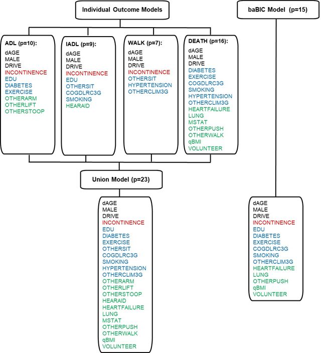
Fig. 3 shows the selection of the common subset of predictors of the Union model using the predictors in the 4
Individual Outcome models of the HRS data. The number of predictors in the Individual Outcome models ranged from
7 to 16. The Union model, which contained all the predictors found in at least 1 of the 4 Individual Outcome models,
had 23 predictors, and most of them came from 1 or 2 Individual Outcome models. By contrast, the baBIC model with
15 predictors was more parsimonious than the Union model, and all the predictors selected in the baBIC model were
also present in the Union Model. These results were also con rmed in the simulation study. In both scenarios with
correlated and uncorrelated outcomes, the Union model had on average more predictors than the baBIC model (Table
1). The difference in the numbers of predictors between Union and baBIC models was more subtle in scenario 1 where
the simulated survival times were generated using the common set of predictors from the baBIC model in the HRS
data (correlated outcomes Union model 15.45 [SE: 0.03] vs. baBIC model 13.15 [SE: 0.04]; uncorrelated outcomes
Union model 15.62 [SE: 0.04] vs. 13.46 [SE: 0.04]). In contrast, scenario 2—where the survival times were obtained
using the individual best sets of predictors of the HRS data—showed a more evident difference between the Union and
baBIC models (correlated outcomes Union model 21.62 [SE: 0.06] vs. baBIC model 13.67 [SE: 0.06]; uncorrelated
outcomes Union model 21.91 [SE: 0.05] vs. 14.01 [SE: 0.05]).
In the HRS data and simulations with correlated and uncorrelated outcomes, the C-statistics of the Individual
Outcome, Union, and baBIC models were clinically similar within each outcome. The average C-statistics across
outcomes of the Union and the baBIC models were also comparable in the HRS data (0.662 vs. 0.657 respectively). In
the simulations, the average predictive accuracies of the Union and baBIC models were very similar regardless of the
scenario and the correlation among the outcomes (e.g. scenario 2, correlated outcomes, Union model: 0.650 [SE:
0.0002] vs. baBIC model 0.644 [SE: 0.0002]) (Table 2).
As shown in Table 1, the average number of predictors of the baBIC models obtained across both simulation
scenarios with correlated and uncorrelated outcomes were slightly smaller than the 15 predictors obtained in the
baBIC model of the HRS data. However, the average C-statistics of the baBIC models of both simulation scenarios
with correlated and uncorrelated outcomes were very similar to the C-statistic of the baBIC model of the HRS data (e.g.
scenario 2, correlated outcomes: 0.664 [SE: 0.0002] vs. HRS data: 0.657) (Table 2).
When using the baBIC method in the simulations, most of the predictors present in the baBIC model of the HRS data
were correctly identi ed 80% of the times or more. On average in scenario 1, this method selected the same (correct)
predictor as in the HRS data 85.7% of the times for correlated outcomes and 88.1% of the times for uncorrelated
outcomes. In simulation scenario 2, the baBIC method selected on average the correct predictors 79.1% of the times
Page 7/28for correlated outcomes and 82.4% of the times for uncorrelated outcomes. In the simulations, the number of correct
predictors in the baBIC models ranged from 9 to 15 (15 being the maximum possible), and the percentage of models
with 13 or more predictors ranged from 42.8% (scenario 2, correlated outcome) to 89.4% (scenario 1, uncorrelated
outcomes). In Scenario 2, the predictors selected in the Union model, but not in the baBIC model of the HRS data, were
included in the simulations less than 25% of the times, whereas these predictors were almost never present in
simulations of scenario 1. Finally, the percentage of predictors not included in either the baBIC or Union models of
HRS but present in the baBIC models of the simulations was less than 6% across scenarios (Table 3).
Discussion
The baBIC selection method produced a model with a good balance between parsimony and predictive accuracy. In
both the HRS data and the simulations, this model was more parsimonious than the Union model, and it showed
minimal loss of predictive discrimination. A good compromise between parsimony and accuracy is important since
models that are simpler to understand and explain and that predict outcomes well are more likely to be implemented.
Models with too few predictors cannot adequately describe the relationship between outcomes and predictors,
whereas those with too many predictors can cause over tting problems. Moreover, as the number of predictors in the
model increases, the time and cost of collecting them could also increase. From a practical perspective, busy
clinicians are unlikely to use a prognostic model with a daunting list of predictors to collect and enter. Although we did
not formally incorporate a penalization associated with the cost of the predictors, other authors have explicitly
balanced predictive accuracy against cost of the predictors (12).
In scenario 1, where the simulated survival times were generated using only the common set of predictors from the
original baBIC model, the simulated baBIC models were still more parsimonious than the simulated Union models (by
about 2 predictors on average). The selection method intrinsically favored the predictors that were used during the
data-generating mechanism. Consequently, during the individual selection process, the 4 outcomes ended up having
more common predictors, which in turn reduced the overall number of predictors in the Union model. On the other
hand, scenario 2 assumed that each outcome had an individual best set of predictors, markedly increasing the
number of predictors in the simulated Union models while maintaining comparable parsimony in the simulated baBIC
models to those from scenario 1.
In the simulations, we found that the baBIC method performed well by selecting on average a high percentage of the
predictors included in the nal baBIC model of the HRS data (i.e. high percentage of correct inclusion), while keeping a
low percentage of the predictors that were not in the baBIC model (i.e. high percentage of correct exclusion). In
simulation scenario 2, the predictors included in the Union model, but not in the baBIC model of the HRS data showed
up in the simulations less than 25% of the times. This was expected since these predictors were used during the
simulation of the outcomes, and consequently they were partially favored during the selection method.
The average number of predictors of the nal models of the simulations was slightly smaller than that of the nal
models of the HRS data. This could be explained because our attempt to replicate the structure of the HRS data did
not entirely capture its complexity. Despite this, the average C-statistic of the nal models of the simulations and the
HRS data were clinically similar.
Breiman and Friedman (37) considered the relationship between the outcomes to improve predictive accuracy. In this
way, several studies have developed methods for variable selection explicitly accounting for the correlation among
multiple outcomes (10, 11, 13, 38, 39). In our method, we did not include the between-outcomes correlation. However,
by averaging the normalized BIC across outcomes and selecting the best subset of predictors based on the minimum
Page 8/28average normalized BIC, we pooled evidence across outcomes and implicitly incorporated their relationships.
Furthermore, in the simulation study, we found that the percentage of correct inclusion of predictors (compared with
the predictors selected in the baBIC model of the HRS data) was similar within the same simulation scenario with
correlated and uncorrelated outcomes. These ndings suggest that during variable selection a similar subset of
predictors can be obtained regardless of the correlation among the outcomes.
As noted, several studies have used penalized regression under the high dimensional multivariate regression setting,
where the numbers of predictors and outcomes may be large compared to the sample size. Regularization methods
are particularly suitable for the study of genetic pathways or genome-wide association analysis, where high
dimension, low sample size settings are very common (10, 15, 38, 39). In clinical settings, researchers are usually
interested in interpretable effect estimates in addition to good predictive performance. Regression coe cients
estimated by regularization schemes like those that are an extension of LASSO can be biased, making their
interpretation more di cult (40). Furthermore, in our case-study data we obtained less parsimonious Individual and
Union models with LASSO selection compared to backward elimination, while maintaining very similar predictive
accuracy. Likewise, in an extensive simulation study, Hastie et al. (29) have recently noted that neither LASSO nor best
subset selection nor stepwise regression was dominant across a variety of problem settings, and that no method had
a large difference in variation explained. Thus, they suggested favoring methods that are easy to compute.
Consequently, we believe that in the clinical practice where the sample size is usually large compared with the number
of outcomes and predictors, our baBIC method, which extends the use of popular (non-regularized) variable selection
methods to the multivariate settings, has the bene t of easier implementation and interpretation as well as good
predictive performance and parsimony.
As in our study, other authors have extended stepwise methods and criterion-based selection to multivariate settings
(41-43). Our method differs in that we combined backward elimination with a criterion-based selection method like the
BIC. By doing this, we improved computational e ciency by not tting all possible models—as traditional criterion-
based selection methods do—while maintaining predictive performance by using BIC instead of statistical signi cance
(i.e. traditional stepwise methods), which does not always indicate predictive value (44).
More recently, a clinical study identi ed a common set of predictors across several adverse outcomes (45). The
authors identi ed the predictors that were signi cantly associated with most or all the outcomes, one of them being a
composite of the other outcomes. This method is simple to implement and allows optimizing clinical resources by
focusing on a single-combined outcome. However, the authors relied on more ad-hoc strategy to identify the common
set of predictors, whereas our approach focuses on selecting the best subset of predictors based on minimizing an
extension of the BIC.
It is worth mentioning that our method focused on one of the rst steps of building a regression model. That is, we
aimed to select a common subset of variables from a pool of many available predictors rather than identify a nal
predictive model. Thus, we assumed that all aspects of model building are xed, except the selection of the predictors.
In the actual application of this method, researchers will need to consider the rest of the aspects involved in model
building; for example, possible inclusion of non-linear terms, interaction and multicollinearity between predictors, and
for survival models, validity of the proportional hazard assumption. Additionally, it will be important to assess the
performance of the nal model using both calibration and discrimination techniques, as well as conducting model
validation by internal cross validation (bootstrapping) and external validation. In a real life application, our method
could be fully incorporated during the process of model development and validation.
Page 9/28Conclusions
Our baBIC method implemented a straightforward approach to obtain a common set of variables for the prediction of
several outcomes. By selecting a common set of predictors for multiple clinical outcomes, researchers will be able to
build prognostic models that are both accurate and parsimonious, potentially saving the clinical time and expense
associated with gathering additional unnecessary predictors. Although the method shown here was developed for
survival data using BIC as a convenient statistic for selection, it could easily be extended to generalized linear models
or other information criteria such as the AIC. Moreover, this method can potentially be applied to larger data with a
greater number of predictors and outcomes. And under this setting, it would be worth exploring further the
implementation of the baBIC method into the LASSO framework. As the number of predictors and outcomes
increases, there would be some computational challenges particularly for Competing-risk survival models that have
longer run time than other regression models.
List Of Abbreviations
AIC: Akaike Information Criterion
ADL: Activities of Daily Living
baBIC: Best Average BIC model
BIC: Bayesian Information Criterion
SE: Standard Error
C-statistic: Concordance statistic
HRS: Health and Retirement Study
IADL: Instrumental Activities of Daily Living
nBIC: normalized BIC
Declarations
Ethics approval and consent to participate
Before each interview, HRS participants are provided with a written informed consent information document and give
oral consent for their participation in the HRS. The institutional review boards of the University of California, San
Francisco, and the San Francisco Veterans Affairs Medical Center approved the present study.
Consent for publication
Not applicable
Availability of data and materials
All data generated or analyzed during this study, and the codes used to generate the results of this article are included
within the article and its additional les.
Page 10/28Competing interests
The authors declare that they have no competing interests.
Funding
This work was supported by the National Institute on Aging (grant numbers: R01 AG047897, R01 AG057751). The
funding agency did not participate in the design of the study, collection, analysis, interpretation of data, or in writing
the manuscript.
Authors' contributions
LGDR drafted the manuscript, had full access to all the data in the study and took responsibility for the integrity of the
data and the accuracy of the data analysis. SJL, AKS, and WJB designed the study and directed its implementation.
SG helped on the acquisition and analysis of the data. All authors read and approved the nal manuscript.
Acknowledgments
The authors thank Regina Anavy for proofreading the article.
References
1. Akaike H. Information theory and an extension of the maximum likelihood principle. In: Petrov BN, Csaki F, editors.
Second international symposium on information theory. Budapest, Hungary: Akadémiai Kiado;1973. p. 267 – 81.
https://link.springer.com/chapter/10.1007/978-1-4612-1694-0_15.
2. Schwarz G. Estimating the dimension of a model. Ann Statist. 1978;6:461 – 4.
http://doi.org/10.1214/aos/1176344136.
3. Steinhauser KE, Christakis NA, Clipp EC, McNeilly M, McIntyre L, Tulsky JA. Factors considered important at the
end of life by patients, family, physicians, and other care providers. JAMA 2000;284:2476 – 82.
https://doi.org/10.1001/jama.284.19.2476.
4. Fried TR, Bradley EH, Towle VR, Phil M, Allore H. Understanding the treatment preferences of seriously ill patients.
N Engl J Med. 2002;346:1061 – 66. https://doi.org/10.1056/NEJMsa012528.
5. Singer DE, Chang Y, Fang MC, et al. The net clinical bene t of warfarin anticoagulation in atrial brillation. Ann
Intern Med. 2009;151:297 – 305. https://doi.org/10.7326/0003-4819-151-5-200909010-00003.
6. Fang MC, Go AS, Chang Y, et al. A new risk scheme to predict warfarin-associated hemorrhage. J Am Coll Cardiol.
2011;58:395 – 401. https://doi.org/10.1016/j.jacc.2011.03.031.
7. Kirkman MS, Briscoe VJ, Clark N, et al. Diabetes in older adults: a consensus report. J Am Geriatr Soc.
2012;60:2342 – 56. https://doi.org/10.1111/jgs.12035.
8. American Geriatrics Society Expert Panel on Care of Older Adults with Diabetes Mellitus, Moreno G, Mangione CM,
Kimbro L, Vaisberg E. Guidelines abstracted from the American Geriatrics Society Guidelines for Improving the
Care of Older Adults with Diabetes Mellitus: 2013 update. J Am Geriatr Soc. 2013;61:2020 – 6.
https://doi.org/10.1111/jgs.12514.
9. Turlach BA, Venables WN, Wright SJ. Simultaneous variable selection. Technometrics 2005;47:349 – 63.
https://doi.org/10.1198/004017005000000139.
10. Kim S, Sohn K-A, Xing EP. A multivariate regression approach to association analysis of quantitative trait network.
Bioinformatics 2009;25:i204 – i212. https://doi.org/10.1093/bioinformatics/btp218.
Page 11/2811. Rothman AJ, Levina E, Zhu J. Sparse multivariate regression with covariance estimation. J Comput Graph Statist
2010;19:947 – 962. https://doi.org/10.1198/jcgs.2010.09188.
12. Brown PJ, Fearn T, Vannucci M. The choice of variables in multivariate regression: A non-conjugate Bayesian
decision theory approach. Biometrika 1999;86:635 – 48. https://doi.org/10.1093/biomet/86.3.635.
13. Lee KH, Tadesse MG, Baccarelli AA, Schwartz J, Coull BA. Multivariate Bayesian variable selection exploiting
dependence structure among outcomes: Application to air pollution effects on DNA methylation. Biometrics
2016;73:232 – 41. http://doi.org/doi:10.1111/biom.12557.
14. Kundu D, Mitra R, Gaskins JT. Bayesian Variable Selection for Multi-Outcome Models Through Shared Shrinkage.
Scand J Stat. 2019. https://arxiv.org/abs/1904.11594v1.
15. Peng J, Zhu J, Bergamaschi A, et al. Regularized Multivariate Regression for Identifying Master Predictors with
Application to Integrative Genomics Study of Breast Cancer. Ann Appl Statist.2010;4:53 – 77.
http://doi.org/10.1214/09-AOAS271SUPP.
16. University of California San Francisco: Repository of published geriatric prognostic indices,
https://www.eprognosis.org/; 2019 [accessed 1 Apr 2020].
17. Yourman LC, Lee SJ, Schonberg MA, Widera EW, Smith AK. Prognostic indices for older adults. A systematic
Review. JAMA 2012;307:182 – 92. https://doi.org/10.1001/jama.2011.1966.
18. Lee SJ, Lindquist K, Segal MR, Covinsky KE. Development and validation of a prognostic index for 4-year
mortality in older adults. JAMA 2006;295:801 – 8. https://doi.org/10.1001/jama.295.7.801.
19. Cruz M, Covinsky K, Widera EW, Stijacic-Cenzer I, Lee SJ. Predicting 10-Year Mortality for Older Adults. JAMA
2013;309:874 – 6. https://doi.org/10.1001/jama.2013.1184.
20. Schonberg MA, Davis RB, McCarthy EP, Marcantonio ER. Index to predict 5-year mortality of community dwelling
adults aged 65 an older using data from the National Health Interview Survey. J Gen Intern Med. 2009;24:1115 –
22. https://doi.org/10.1007/s11606-009-1073-y.
21. Schonberg MA, Davis RB, McCarthy EP, Marcantonio ER. External validation of an index to predict up to 9-year
mortality of community-dwelling adults aged 65 and older. J Am Geriatr Soc. 2011;59:1444 – 51.
https://doi.org/10.1111/j.1532-5415.2011.03523.x.
22. Sonnega A, Faul JD, Ofstedal MB, Langa KM, Phillips JW, Weir DR. Cohort pro le: the Health and Retirement
Study (HRS). Int J Epidemiol. 2014;43:576 – 85. https://doi.org/10.1093/ije/dyu067.
23. Health and Retirement Study, (Cross-Wave Tracker File 2014 Final, Version 1.0) public use data set. Produced and
distributed by the University of Michigan with funding from the National Institute on Aging (grant number NIA
U01AG009740). Ann Arbor, MI, (2017).
24. Health and Retirement Study, (RAND HRS Data, Version P) public use data set. Produced and distributed by the
University of Michigan with funding from the National Institute on Aging (grant number NIA U01AG009740). Ann
Arbor, MI, (2016).
25. RAND HRS Data, Version P. Produced by the RAND Center for the Study of Aging, with funding from the National
Institute on Aging and the Social Security Administration. Santa Monica, CA (August 2016).
26. Cox DR. Regression models and life tables. J R Stat Soc Series B 1972;34:187-220.
https://www.jstor.org/stable/2985181.
27. Fine JP, Gray RJ. A proportional hazards model for the subdistribution of a competing risk. J Am Stat Assoc
1999;94:496 – 509. https://doi.org/10.1080/01621459.1999.10474144.
28. Tibshirani R. Regression shrinkage and selection via the lasso. J Roy Statist Soc Ser B 1996;58:267 – 88.
jstor.org/stable/2346178.
Page 12/2829. Hastie T, Tibshirani R, Tibshirani R. Best Subset, Forward Stepwise, or Lasso? Analysis and Recommendations
Based on Extensive Comparisons. Stat Sci in press. https://www.stat.cmu.edu/~ryantibs/papers/bestsubset.pdf.
30. Zhou H, Hastie T, Tibshirani R. On the “degrees of freedom” of the LASSO. Ann Statist. 2007;35:2173-92.
https://doi.org/10.1214/009053607000000127.
31. Ahrens A, Hansen CB, Schaffer ME. lassopack: Model selection and prediction with regularized regression in
Stata. Stata Journal 2020;20:176-235. https://doi.org/10.1177/1536867X20909697.
32. Steyerberg EW, Eijkemans MJC, Harrell FE, Habbema JDF. Prognostic modelling with logistic regression analysis:
a comparison of selection and estimation methods in small data sets. Stat Med. 2000;19:1059 – 79.
https://doi.org/10.1002/(SICI)1097-0258(20000430)19:83.0.CO;2-0.
33. Steyerberg EW. Disadvantages of Stepwise Methods. In: Gail M, Tsiatis A, Krickeberg K, Wong W, Sarnet J, editors.
Clinical Prediction Models. A Practical Approach to Development, Validation, and Updating. Springer; 2009. p.
197-204.
34. Harrell FE. Regression Modeling Strategies. With Applications to Linear Models, Logistic and Ordinal Regression,
and Survival Analysis. 2nd ed. Springer; 2015.
35. Harrell FE. The PHGLM Procedure. In: SUGI Supplemental Library Users Guide; 1986 Version 5 Edition:437-466.
SAS Institute Inc., Cary, NC.
36. Wolbers M, Koller MT, Witteman JC, Steyerberg EW. Prognostic models with competing risks: methods and
application to coronary risk prediction. Epidemiology 2009;20:555 – 61.
https://doi.org/10.1097/EDE.0b013e3181a39056.
37. Breiman L, Friedman JH. Predicting multivariate responses in multiple linear regression. J R Statist Soc Series B
1997;59:3 – 54. https://doi.org/10.1111/1467-9868.00054.
38. Sofer T, Dicker L, Lin X. Variable selection for high dimensional multivariate outcomes. Stat Sin 2014;24:1633 –
54. http://doi.org/10.5705/ss.2013.019.
39. Zhang H, Zheng Y, Yoon G, et al. Regularized estimation in sparse high-dimensional multivariate regression, with
application to a DNA methylation study. Stat Appl Genet Mol Biol 2017;16:159 – 71.
https://doi.org/10.1515/sagmb-2016-0073.
40. Heinze G, Wallisch C, Dunkler D. Variable selection - A review and recommendations for the practicing statistician.
Biom J. 2018;60:431 –49. http://doi.org/10.1002/bimj.201700067.
41. Bedrick EJ, Tsai C. Model Selection for Multivariate Regression in Small Samples. Biometrics. 1994;50:226 – 31.
http://doi.org/10.2307/2533213.
42. Fujikoshi Y, Satoh K. Modi ed AIC and Cp in Multivariate Linear Regression. Biometrika 1997;84:707 – 16.
https://doi.org/10.1093/biomet/84.3.707.
43. Al-Subaihi AA. Variable Selection in Multivariable Regression Using SAS/IML. J Stat Softw. 2002;07(12).
http://doi.org/10.18637/jss.v007.i12.
44. Lo A, Chernoff H, Zheng T, Lo SH. Why signi cant variables aren’t automatically good predictors. PNAS
2015;112:13892 – 97. https://doi.org/10.1073/pnas.1518285112.
45. Kabue S, Liu V, Dyer W, Raebel M, Nichols G, Schmittdiel J. Identifying Common Predictors of Multiple Adverse
Outcomes Among Elderly Adults With Type-2 Diabetes. Med Care 2019;57:702 – 709.
Tables
Table 1. Comparison of Number of Predictors Using HRS Data and Simulations with Correlated and Uncorrelated Outcomes
Page 13/28Data Individual Outcome Models Union Model baBIC Model
Time to first Time to first Time to first Time to death
ADL IADL mobility
dependence difficulty dependence
HRS data, 10.0 9.0 7.0 16.0 23.0 15.0
Number of
Predictors
Simulations, Number of predictors Mean [Monte Carlo Standard Error]
Scenario 1 correlated 8.63 [0.05] 7.03 [0.04] 6.17 [ 0.05] 12.96 [0.03] 15.45 [0.03] 13.15 [0.04]
uncorrelated 8.55 [0.05] 7.04 [0.04] 6.08 [0.05] 13.03 [0.03] 15.62 [0.04] 13.46 [0.04]
Scenario 2 correlated 8.47 [0.04 ] 7.77 [0.04 ] 6.03 [0.04 ] 15.00 [0.04 ] 21.62 [0.06 ] 13.67 [0.06]
uncorrelated 8.45 [0.04 ] 7.76 [0.04 ] 6.00 [0.04 ] 14.91 [0.04] 21.91 [0.05] 14.01 [0.05]
Legend:
ADL: Activities of Daily Living
baBIC Model: Best Average BIC model, best subset of predictors based on the minimum average normalized BIC across the 4
outcomes
BIC: Bayesian Information Criterion
correlated: simulated data with correlated outcomes
HRS: Health and Retirement Study
IADL: Instrumental Activities of Daily Living
Individual Outcome Model: Best subset of predictors based on the minimum BIC for each individual outcome
Scenario 1: simulated data generated using common subset of predictors obtained in the baBIC model of the HRS data for all
outcomes
Scenario 2: simulated data generated using sets of predictors obtained in the Individual Outcome models of the HRS data
uncorrelated: simulated data with uncorrelated outcomes
Union Model: Subset of all the predictors that were in at least 1 of the 4 best subsets of predictors based on the minimum BIC for
each individual outcome
Table 2. Comparison of Harrell’s C-statistic Using HRS Data and Simulations with Correlated and Uncorrelated Outcomes
Page 14/28Outcome Data Individual Union Model baBIC Model
Outcome Model
Time to first ADL HRS data, C- 0.6391 [0.0064] 0.6475 [0.0063] 0.6411 [0.0064]
dependence statistic [Standard
Error]
Simulations, C-statistic Mean [Monte Carlo Standard Error]
Scenario 1 correlated 0.6276 [0.0003] 0.6329 [0.0003] 0.6301 [0.0003 ]
uncorrelated 0.6268 [0.0003] 0.6324 [0.0003] 0.6299 [0.0003]
Scenario 2 correlated 0.6230 [0.0003 ] 0.6269 [0.0003 ] 0.6209 [0.0003]
uncorrelated 0.6235 [0.0003 ] 0.6273 [0.0003 ] 0.6211 [0.0003]
Time to first IADL HRS data, C- 0.6355 [0.0063] 0.6380 [0.0063] 0.6350 [0.0063 ]
difficulty statistic [Standard
Error]
Simulations, C-statistic Mean [Monte Carlo Standard Error]
Scenario 1 correlated 0.6245 [0.0003] 0.6288 [0.0003] 0.6269 [0.0003]
uncorrelated 0.6238 [0.0003] 0.6280 [0.0003] 0.6264 [0.0003 ]
Scenario 2 correlated 0.6258 [0.0003 ] 0.6293 [0.0003 ] 0.6253 [0.0003]
uncorrelated 0.6251 [0.0003 ] 0.6287 [ 0.0003] 0.6247 [0.0003]
Time to first HRS data, C- 0.6351 [0.0085] 0.6487 [0.0084] 0.6432 [0.0085]
mobility statistic [Standard
dependence Error]
Simulations, C-statistic Mean [Monte Carlo Standard Error]
Scenario 1 correlated 0.6329 [0.0004] 0.6416 [0.0004] 0.6390 [ 0.0004]
uncorrelated 0.6330 [0.0004] 0.6416 [0.0004] 0.6393 [0.0004 ]
Scenario 2 correlated 0.6306 [ 0.0004] 0.6369 [0.0004 ] 0.6296 [0.0004]
uncorrelated 0.6313 [ 0.0004] 0.6376 [0.0004 ] 0.6302 [0.0004]
Time to death HRS data, C- 0.7109 [0.0041] 0.7119 [0.0041] 0.7086 [0.0041]
statistic [Standard
Error]
Simulations, C-statistic Mean [Monte Carlo Standard Error]
Scenario 1 correlated 0.7031 [0.0002] 0.7034 [0.0002] 0.7008 [0.0002 ]
uncorrelated 0.7030 [0.0002] 0.7032 [0.0002] 0.7008 [0.0002]
Scenario 2 correlated 0.7052 [0.0002 ] 0.7056 [0.0002 ] 0.7005 [0.0002]
uncorrelated 0.7050 [ 0.0002] 0.7055 [ 0.0002] 0.7003 [0.0002]
Page 15/28Outcome Data Individual Union Model baBIC Model
Outcome Model
Mean of 4 HRS data, C- 0.6615 0.6570
Outcomes statistic
Simulations, C-statistic Mean [Monte Carlo Standard Error]
Scenario 1 correlated 0.6517 [0.0002] 0.6492 [ 0.0002]
uncorrelated 0.6513 [0.0001] 0.6491 [0.0002]
Scenario 2 correlated 0.6497 [0.0002 ] 0.6441 [0.0002]
uncorrelated 0.6498 [0.0001 ] 0.6441 [0.0002]
Legend:
ADL: Activities of Daily Living
baBIC Model: Best Average BIC model, best subset of predictors based on the minimum average normalized BIC across the 4
outcomes
BIC: Bayesian Information Criterion
correlated: simulated data with correlated outcomes
HRS: Health and Retirement Study
IADL: Instrumental Activities of Daily Living
Individual Outcome Model: Best subset of predictors based on the minimum BIC for each individual outcome
Scenario 1: simulated data generated using common subset of predictors obtained in the baBIC model of the HRS data for all
outcomes
Scenario 2: simulated data generated using sets of predictors obtained in the Individual Outcome models of the HRS data
uncorrelated: simulated data with uncorrelated outcomes
Union Model: Subset of all the predictors that were in at least 1 of the 4 best subsets of predictors based on the minimum BIC for
each individual outcome
Table 3. Percentage of Predictor Inclusion in baBIC model using Simulations with Correlated and Uncorrelated Outcomes
Page 16/28Percentage of Inclusion in Simulations
Scenario 1 Scenario 2
Correlated Uncorrelated Correlated Uncorrelated
Predictors in baBIC Model for original HRS Data
dAGEa 100.0 100.0 100.0 100.0
MALEb 100.0 100.0 100.0 100.0
DRIVE 88.4 97.8 89.2 98.2
INCONTINENCE 83.6 96.6 80.2 94.4
EDU 82.4 85.2 75.2 84.6
DIABETES 100.0 100.0 100.0 100.0
EXERCISE 85.8 94.6 88.0 91.4
COGDLRC3G 100.0 100.0 99.8 100.0
SMOKING 100.0 100.0 100.0 100.0
OTHERCLIM3G 90.6 95.6 61.4 67.6
HEARTFAILURE 93.4 92.4 84.8 84.8
LUNG 52.6 50.2 54.0 53.4
OTHERPUSH 88.8 91.8 78.0 81.2
qBMI 52.8 49.2 24.6 23.4
VOLUNTEER 95.2 92.2 93.0 91.6
Additional predictors in Union Model for original HRS Data
OTHERSIT 0.2 0.0 22.2 16.0
HYPERTENSION 0.0 0.0 21.2 18.0
OTHERARM 0.0 0.0 19.6 21.0
OTHERLIFT 0.0 0.0 16.2 19.2
OTHERSTOOP 0.2 0.0 12.8 15.0
HEARAID 0.2 0.0 3.4 1.2
MSTAT 0.0 0.0 19.8 24.2
OTHERWALK 0.0 0.0 18.2 15.4
Other predictors not present in baBIC or Union models for original HRS data
0.8 0.0 5.6 0.6
Average Percentage of Correctc Inclusion per predictor
85.7 88.1 79.1 82.4
baBIC models with correctc:
9 predictors 0.4
Page 17/28Percentage of Inclusion in Simulations
Scenario 1 Scenario 2
Correlated Uncorrelated Correlated Uncorrelated
10 predictors 0.4 4.8 0.8
11 predictors 2.8 1.8 18.6 7.6
12 predictors 19.4 8.8 33.4 30
13 predictors 42.4 39.2 29.6 44.6
14 predictors 30.2 42.4 11.6 15.8
15 predictors 4.8 7.8 1.6 1.2
13+ predictors 77.4 89.4 42.8 61.6
Legend:
baBIC Model: Best Average BIC model, best subset of predictors based on the minimum average normalized BIC across the 4
outcomes
BIC: Bayesian Information Criterion
COGDLRC3G: number of words from 10-word list recalled correctly after 5 minutes
Correctc: it is defined compared to subset of predictors in baBIC model of HRS data
correlated: simulated data with correlated outcomes
dAGEa (age deciles groups), MALEb (whether male): predictors that are forced into all models
DIABETES: whether has diabetes with and without medicine
DRIVE: whether able to drive
EDU: education 12+ years
EXERCISE: exercise frequency
HEARAID: whether wears hearing aid
HEARTFAILURE: whether has heart failure or others heart problems (e.g. angina, heart attack, heart disease)
HYPERTENSION: whether has hypertension
INCOTINENCE: whether has incontinence
LUNG: chronic lung disease
MSTAT: marital status
OTHERARM: having difficulty reaching above shoulder
OTHERCLIM3G: having difficulty climbing stairs
OTHERLIFT: having difficulty with lifting weights over 10 pounds
OTHERPUSH: having difficulty with pushing large objects
OTHERSIT: having difficulty with sitting for 2 hours
OTHERSTOOP: having difficulty with stooping, kneeling, or crouching
OTHERWALK: having difficulty with walking one block or in the room
Page 18/28qBMI: quintile groups
Scenario 1: simulated data generated using common subset of predictors obtained in the baBIC model of the HRS data for all
outcomes
Scenario 2: simulated data generated using sets of predictors obtained in the Individual Outcome models of the HRS data
SMOKING: whether smokes
uncorrelated: simulated data with uncorrelated outcomes
Union Model: Subset of all the predictors that were in at least 1 of the 4 best subsets of predictors based on the minimum BIC for
each individual outcome
VOLUNTEER: whether helps as volunteer
Additional File Legends
Additional File 1. Comparison of Individual and Union Models of HRS Data using BIC Backward Elimination and
LASSO Selection based on Optimal λ at Minimum BIC
File format: .xls
Legend:
ADL: time to rst Activities of Daily Living (ADL) dependence
ALCOHOL: whether drinks alcohol
ARTHRITIS: whether has arthritis
BIC: Bayesian Information Criterion
CANCER: whether has cancer diagnosed in last 2 years or not
CESDALL: whether depressed
COGDLRC3G: number of words from 10-word list recalled correctly after 5 minutes
COGIMRC3G: number of words from 10-word list recalled correctly
dAGE: age deciles groups
DEATH: time to death
DIABETES: whether has diabetes with and without medicine
DRIVE: whether able to drive
EDU: education 12+ years
EXERCISE: exercise frequency
Page 19/28EYE2G: whether has vision problems
FALL: whether falls with or without injury
HEARAID: whether wears hearing aid
HEARING: hearing ability
HEARTFAILURE: whether has heart failure or others heart problems (e.g. angina, heart attack, heart disease)
HYPERTENSION: whether has hypertension
IADL: time to rst Instrumental Activities of Daily Living (IADL) di culty
INCOTINENCE: whether has incontinence
Individual Outcome Model: Best subset of predictors based on the minimum BIC for each individual outcome
LALONE: whether lives alone
LUNG: chronic lung disease
MALE: whether male
MSTAT: marital status
OTHERARM: having di culty reaching above shoulder
OTHERCHAIR: having di culty getting up from a chair
OTHERCLIM3G: having di culty climbing stairs
OTHERLIFT: having di culty with lifting weights over 10 pounds
OTHERPUSH: having di culty with pushing large objects
OTHERSIT: having di culty with sitting for 2 hours
OTHERSTOOP: having di culty with stooping, kneeling, or crouching
OTHERWALK: having di culty with walking one block or in the room
PAIN: whether has pain
qBMI: quintile groups
qFAGE: quartile groups of age father died or if alive placed in older age group quartile
qMAGE: quartile groups of age mother died or if alive placed in older age group quartile
SHLT: self-rated health
SMOKING: whether smokes
Page 20/28STROKE: whether had stroke with or without remaining problems
Union Model: Subset of all the predictors that were in at least 1 of the 4 best subsets of predictors based on the
minimum BIC for each individual outcome
VOLUNTEER: whether helps as volunteer
WALK: time to rst mobility dependence
Additional File 2. Coe cient Estimates (Standard Errors in parentheses) and Chi-Square Statistics of Predictors used
in Scenarios 1 and 2
File format: .xls
Legend:
ADL: time to rst Activities of Daily Living (ADL) dependence
COGDLRC3G: number of words from 10-word list recalled correctly after 5 minutes
dAGE: age deciles groups
DEATH: time to death
DIABETES: whether has diabetes with and without medicine
DRIVE: whether able to drive
EDU: education 12+ years
EXERCISE: exercise frequency
HEARAID: whether wears hearing aid
HEARTFAILURE: whether has heart failure or others heart problems (e.g. angina, heart attack, heart disease)
HYPERTENSION: whether has hypertension
IADL: time to rst Instrumental Activities of Daily Living (IADL) di culty
INCOTINENCE: whether has incontinence
LUNG: chronic lung disease
MALE: whether male
MSTAT: marital status
OTHERARM: having di culty reaching above shoulder
OTHERCLIM3G: having di culty climbing stairs
Page 21/28You can also read