Noise indicators under the Environmental Noise Directive 2021. Methodology for estimating missing data - Eionet

Eionet Report - ETC/ATNI 2021/6

 Noise indicators under the Environmental
 Noise Directive 2021. Methodology for
 estimating missing data

 July 2021

 Authors:
 Jaume Fons-Esteve (UAB), Francisco Domingues (UAB), Maria José Ramos (UAB)

ETC/ATNI consortium partners:
NILU – Norwegian Institute for Air Research, Aether Limited, Czech
Hydrometeorological Institute (CHMI), EMISIA SA, Institut National de
l’Environnement Industriel et des risques (INERIS), Universitat Autònoma de
Barcelona (UAB), Umweltbundesamt GmbH (UBA-V), 4sfera Innova,
Transport & Mobility Leuven NV (TML)

Eionet Report - ETC/ATNI 2021/6

Cover design: EEA
Layout: ETC/ATNI

Legal notice
The contents of this publication do not necessarily reflect the official opinions of the European Commission or other institutions
of the European Union. Neither the European Environment Agency, the European Topic Centre on Air pollution, transport, noise
and industrial pollution nor any person or company acting on behalf of the Agency or the Topic Centre is responsible for the use
that may be made of the information contained in this report.

Copyright notice
© European Topic Centre on Air pollution, transport, noise and industrial pollution, 2021

Reproduction is authorised, provided the source is acknowledged.
Information about the European Union is available on the Internet. It can be accessed through the Europa server
(www.europa.eu).

The withdrawal of the United Kingdom from the European Union did not affect the production of the report.
Data reported by the United Kingdom are included in all analyses and assessments contained herein, unless otherwise indicated.

Author(s)
Jaume Fons-Esteve, Francisco Domingues, Maria José Ramos (UAB)

ETC/ATNI c/o NILU
ISBN 978-82-93752-29-5

European Topic Centre on Air pollution,
transport, noise and industrial pollution
c/o NILU – Norwegian Institute for Air Research
P.O. Box 100, NO-2027 Kjeller, Norway
Tel.: +47 63 89 80 00
Email: etc.atni@nilu.no
Web : https://www.eionet.europa.eu/etcs/etc-atni

Contents

Summary ........................................................................................................................................ 4
Acknowledgements........................................................................................................................ 5
1 Introduction ........................................................................................................................... 6
2 Input data ............................................................................................................................... 7
3 END agglomerations data: gap filling ..................................................................................... 9
 3.1 Gap filling method for agglomerations- road ................................................................. 9
 3.1.1 Overview ............................................................................................................ 9
 3.1.2 Regression........................................................................................................ 13
 3.1.3 Identify outliers and adjust agglomerations with > 100% people exposed .... 14
 3.1.4 Visual inspection of the relationship between people exposed and number of
 inhabitants ....................................................................................................... 15
 3.1.5 Data subsetting for regression analysis and validation ................................... 16
 3.1.6 Test models...................................................................................................... 17
 3.1.7 Validation ......................................................................................................... 20
 3.1.8 Estimate values for missing data ..................................................................... 21
 3.1.9 Calculate the total people exposed in Europe................................................. 21
 3.1.10 Estimate the people distributed by noise bands ............................................. 21
 3.2 Gap filling method for railway noise, aircraft noise and industrial noise inside
 agglomerations ............................................................................................................. 22
4 END major roads and major railways exposure data outside agglomerations: gap filling .. 25
 4.1 Gap filling method ........................................................................................................ 25
5 END Major airport exposure outside agglomerations: gap filling ........................................ 28
 5.1 Overview ....................................................................................................................... 28
 5.2 A methodology based on estimating the noise contour around runaways ................... 6
 5.2.1 Overview ............................................................................................................ 6
 5.2.2 Data requirements............................................................................................. 7
 5.2.3 Delineation of the runaways and noise contours.............................................. 7
 5.2.4 Detailed description of the methodology ......................................................... 9
 5.2.5 Outcome of the test........................................................................................... 9
 5.3 Summary of the proposed methodology ..................................................................... 10
6 Conclusions .......................................................................................................................... 12
7 Abbreviations ....................................................................................................................... 13
8 References ............................................................................................................................ 14
Annex 1 Summary of regression statsitics (agglomeration road) ................................................ 15
Annex 2 R script to estimate missing data of people exposed to roads inside agglomerations . 16
Annex 3 Reported and delineated contour for Lden 55 dB (major airports) ................................. 50

Eionet Report - ETC/ATNI 2021/6 3

Summary

The Environmental Noise Directive (END) offers a common approach to avoiding and preventing
exposure to environmental noise by reporting noise mapping and action planning. This leads to
reducing the harmful effects of noise and preserving quiet areas. Noise sources, as defined by the
END, include major roads with more than three million vehicle passages a year; major railways with
more than 30 000 train passages per year; major airports with more than 50 000 movements per year
(a movement being a take-off or a landing), excluding those purely for training purposes on light
aircraft; and noise from roads, railways, airports and industries inside of agglomerations - part of a
territory, delimited by the Member State, having a population in excess of 100 000 persons and a
population density such that the Member State considers it to be an urbanised area. It is important to
note that the directive does not set limit values but reporting thresholds.
The END requires Member States to determine the number of people exposed to noise sources, inside
and outside urban areas, and large industrial installations inside urban areas, using 5 dB interval bands
at Lden ≥ 55 dB and at Lnight ≥ 50 dB. The experience of the three reporting cycles of the END, which
started in 2007, has demonstrated substantial delays in delivering noise exposure data. For that
reason, methodologies to estimate missing data have been developed as early as 2013 to have a
complete overview of the extent of the population exposed to the noise sources mentioned above
sources. This report reviews previous methodologies and provides a comprehensive description of the
method to gap-fill missing data in all reported noise sources. In particular, it provides a systematic
approach when regression is required (e.g. estimation of the population exposed to agglomerations
roads based on the number of inhabitants) and explore a new method for major airports based on
estimating the noise contour band when this information is not provided.

Eionet Report - ETC/ATNI 2021/6 4

Acknowledgements

Eulàlia Peris, the EEA project manager, supported the work and provided valuable comments on the
report.

Eionet Report - ETC/ATNI 2021/6 5

1 Introduction
The Environmental Noise Directive (END) (EU, 2002) offers a common approach to avoiding and
preventing exposure to environmental noise by reporting noise mapping and action planning, thereby
reducing its harmful effects and preserving quiet areas. Noise sources, as defined by the END, include
major roads with more than three million vehicle passages a year; major railways with more than 30
000 train passages per year; major airports with more than 50 000 movements per year (a movement
being a take-off or a landing), excluding those purely for training purposes on light aircraft; and noise
from roads, railways, airports and industries inside of agglomerations -part of a territory, delimited by
the Member State, having a population in excess of 100 000 persons and a population density such
that the Member State considers it to be an urbanised area. It is important to note that the directive
does not set limit values but reporting thresholds.
The END requires the Member States to determine the number of people exposed to the noise
sources, inside and outside urban areas, and large industrial installations inside urban areas using 5
dB interval bands at Lden ≥ 55 dB and at Lnight ≥ 50 dB. The experience of the three reporting cycles of
the END (2007, 2012, 2017) has demonstrated substantial delays in the reporting of the Member
States, a consequence of a learning process dealing with the complexity of the reporting and the END
requirements. For that reason, methodologies to estimate missing data have been developed as early
as 2013 (Jones, 2013) to have a complete overview of the extent of the population exposed to the
noise sources.
The latest update of the methodology was reported by Ramos (2019), where the need for some
improvements was identified -and out of the scope of the work at that time. The current report tackles
the following issues to improve the methodology and systematise the estimation of the missing data:
 • Provide a systematic approach to test alternative regression models when pertinent (e.g.
 population exposed to roads inside agglomerations).
 • Specify the methodology for the propagation of errors, leading to figures of total people
 exposed with the corresponding confidence interval.
 • Improvements on the estimation of people exposed to noise from major airports based on
 the estimation of the noise contour for Lden 55 dB.
This methodological report summarises the steps followed to obtain estimated results of a complete
noise exposure covering the END sources.

Eionet Report - ETC/ATNI 2021/6 6

2 Input data
This report is based on the review of the methodology developed in 2019 (Ramos, 2019). Therefore,
the same data source has been used, for comparability reasons, when data was required to test some
improvements. The data covers the data reported until 01/01/2019(1).
In order to facilitate the implementation of the workflow for estimating missing data, the minimum
data requirements are specified in Table 2.1, Table 2.2, and Table 2.3 for the different noise sources.
Therefore, a preliminary step is to extract the needed information from the internal noise database(s),
which compile the reported data. The most critical part is the identification of completeness for major
roads and major rails. The objective of this report is out of the scope of the preliminary data selection
-details are available at Ramos (2019). Moreover, changes in the data model implemented in
Reportnet 3.0 may facilitate selecting the needed data. For that reason, Table 2.1, Table 2.2, and Table
2.3 are provided as a reference for futures use.
It should be noted that the methodology also requires data from the previous reporting cycle. The
notation used in this report to generalise the method, is detailed as follows:
 • tn, data from the current reporting cycle
 • tn-1, data from the previous reporting cycle.

Table 2.1: Structure of the input data for people exposed to noise from roads inside agglomerations
 Field Type of data Comment
 Country String
 Country2 String
 Agglomeration_name String
 RLID String
 UniqueAgg_ID String
 Year Integer Reference year of the reported data
 Population Integer
 Lden per noise band Integer -1 not applicable, -2 not available (reported), -
 9999 not reported
 Lnight per noise band Integer -1 not applicable, -2 not available (reported), -
 9999 not reported

Table 2.2: Structure of the input data for people exposed to noise from major airports
 Field Type of data Comment
 Country String
 Mair_name String
 ICAO_code String
 Year Integer Reference year of the reported data
 Lden per noise band Integer -1 not applicable, -2 not available (reported), -
 9999 not reported
 Lnight per noise band Integer -1 not applicable, -2 not available (reported), -
 9999 not reported

(1) https://forum.eionet.europa.eu/etc-atni-consortium/library/subvention-2019/task-deliveries-action-plan-2019/task-
1.1.5.1-noise-data-operational-compilation-and-management/subtask-1.1-update-database-cws/datasets

Eionet Report - ETC/ATNI 2021/6 7

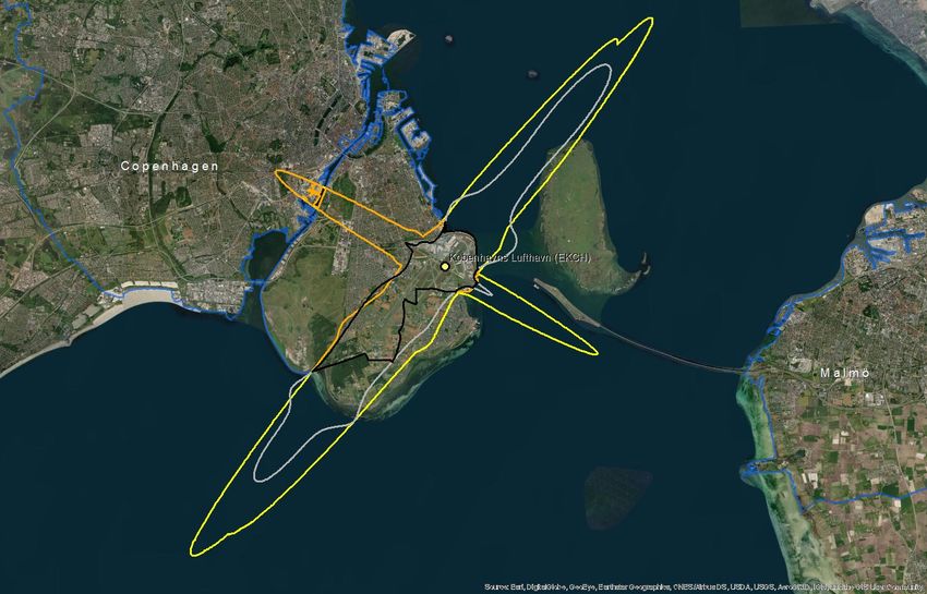
Table 2.3: Structure of the input data for people exposed to noise from major roads and major rails
 Field Type of data Comment
 Country String
 Country2 String
 Unique identifier(s) String (Several All needed fields that provide the unique link to
 fields) the noise database
 Completeness String Complete, partial, not applicable, not provided
 Year Integer Reference year of the reported data
 Lden per noise band Integer
 Lnight per noise band Integer

Eionet Report - ETC/ATNI 2021/6 8

3 END agglomerations data: gap filling

3.1 Gap filling method for agglomerations- road

3.1.1 Overview
This method is based on the working paper “Establishing a methodological proposal to interpolate a
complete coverage on noise exposure at the EU level” (ETC/ACM, 2015), with some improvements
described by Ramos (2019).
Figure 3.1 provides an overview of the process for estimating missing data adapted from Ramos
(2019). In each step, the decision tree uses the best approach according to the available ancillary data:
 • Use data from the previous reporting period if available.
 • When this information is also missing, the following steps are taken:
 o People exposed is estimated with regression analysis, being the number of
 inhabitants the independent variable.
 o Finally, estimate the distribution of the population exposed by noise bands applying
 the European average.
A more detailed explanation and the basis for the methodology applied in each step is provided in
Table 3.1.
The gap-filling methodology also includes those few cases where data is missing for some noise bands.
Then, partial gap filling is conducted as follows:
 • Use data from the previous reporting period for the missing noise band(s).
 • If data from the previous reporting period is not available use the European average of % of
 the population exposed by noise band to estimate the missing data. Table 3.2 provides an
 example of a partial gap-filling when data from the previous period is not available.
The following sections focus on those aspects that were not documented on previous reports:
 • Selection of the appropriate regression model
 • Estimation of the missing data with the corresponding error (error of the prediction).
 • Calculation of the people exposed in Europe as sum of all the agglomerations (reported and
 gap filled). Calculation of the propagation of error as a result of adding individual values with
 their own error (error of the prediction).
 • Estimate the distribution of total noise exposure by noise bands and associated error -error
 of the function’s sum and error to distribute the total by noise bands.
All these steps have been implemented in R to ensure the traceability and replicability of the whole
process, including the assessment of different regression models.

Eionet Report - ETC/ATNI 2021/6 9

Table 3.1: Methods used on the various steps of gap filling people exposed to noise from roads inside agglomerations. Numbers refer to the steps
 highlighted in Figure 3.1
 Step Method for gap filling Explanation Comment
 1 Use the data delivered in the A comparative analysis described in Fons et al. (2017) concluded The method is constrained to the availability of the data on the
 previous reporting period for the that this is the method with the smaller error. previous reporting cycle.
 same agglomeration, if available.
 2 Exclude outliers from the Outliers from the percentage of change between tn-1 and tn based on Previous assessments have identified some extreme population
 reported data to be used for the the interquartile range (IQR, the difference between 3rd and 1st changes exposed to noise between two reporting periods (Ramos,
 regression (step 4) quartile). The exact threshold is ± 1,5 IQR. 2019). Therefore, the estimation of missing data in 2019 (Ramos,
 2019), adopted a methodology to exclude outliers.
 3 Estimate the total population If the country reported the agglomeration's delineation, the The reporting cycle of the Urban Atlas is always one year later than
 from ancillary data. population could be derived from Urban Atlas described in Fons et the END.
 al. (2015). The average error of the estimation based on Urban Atlas
 is 3%, ranging from 1 to 10%. If the delineation has not been
 reported, data from Eurostat can be used. The agglomeration
 population is the independent variable of the regression (step 3) to
 estimate the population exposed when data from the previous
 reporting cycle is not available.
 4 Estimate the population exposed The regression and correlation analysis between population exposed The current report provides a detailed description of the metrics to
 from the regression between and potential predictors (total population, area,…) is documented in evaluate the best regression model, including estimating the error and
 population exposed and Fons et al. (2015). Later on, Fons et al. 2017) demonstrated that, if confidence interval in the final aggregation of data (EU figures). There
 population of the available, using data from the previous reporting period (step 1) is is no a priory regression model to be applied each time that the gap
 agglomeration. more accurate than the regression approach. filling is developed. The regression model needs to be checked each
 time since the relationship is strongly dependent on the data included
 for the regression.
 5 Estimate the % of the population Based on the total number of people exposed per each reported Initially, the % was calculated on a country basis when were enough
 exposed per noise bands (%) agglomeration, we calculate the percentage that each noise band agglomerations reported. The assessment was done in Fons et al.
 from the European average represent versus the total number of people exposed, for Lden and (2017) highlights that using the country average has a similar error
 for Lnight. Then we derive the mean at European level. This approach than the European average. Therefore, it was decided to use in all
 is discussed in depth in Fons et al. (2015). cases the European average for simplicity.

Eionet Report - ETC/ATNI 2021/6 10

Figure 3.1: Overview of the process for estimating the population exposed to roads inside agglomerations when data is not available. The methodology only
 applies to agglomerations that have to report according to END requirements. Numbers indicate specific methods for gap filling depending on
 available ancillary data -details are described in Table 3.1. Source: updated from Ramos (2019)

Eionet Report - ETC/ATNI 2021/6 11

Table 3.2: Example of partial gap-filling when data is missing for some noise bands. N.d., no data
 reported (missing data)
 Lden dB bands 55-59 60-64 65-69 70-74 >75
 Reported data 11.7680 6.000 1.500 n.d. n.d.
 % of people exposed distributed by
 45,8 28,3 18,3 7,0 0,6
 noise band (European average)
 Reported + gap filled data (italics) 11.7680 6.000 1.500 9.500 800

Eionet Report - ETC/ATNI 2021/6 12

3.1.2 Regression
The regression procedure could be summarised as follows:
 1. Identify outliers from the percentage of change of the people exposed between current
 reporting period (tn) and the previous reporting cycle (tn-1).
 2. Plot Lden against the number of inhabitants to visually inspect the most suitable regression
 model. Since it is not always obvious which is the best model, the most plausible ones are
 retained and tested.
 3. Transform the data if it improves the linearity (the most common transformation in previous
 assessments was log transformation).
 4. Divide the data in two groups to test different regression models: one group is used to run the
 regressions, and the second group is used to validate the models.
 5. Calculate the regression model and analyse the corresponding statistics.
 6. Estimate the number of people exposed on the validation subset and compare results
 between different models.
 7. Apply the selected model to the missing data
 8. Calculate the total people exposed in Europe with the confidence interval corresponding to
 the estimated data.
Each step is further described in the following sections. We have used the estimation of population
exposed to Lden to illustrate the methodology. The same approach could be followed in other sources
and Lnight when required.

Eionet Report - ETC/ATNI 2021/6 13

3.1.3 Identify outliers and adjust agglomerations with > 100% people exposed
Previous assessments have identified some extreme cases of change of population exposed to noise
between two reporting periods (Ramos, 2019). Therefore, the estimation of missing data in 2019
(Ramos, 2019), adopted a methodology to exclude outliers. This methodology is based on the
interquartile range (difference between 3rd and 1st quartile).
Figure 3.2 illustrates the distribution of both outliers and non-outliers for the percentage of change of
population exposed to Lden from roads inside agglomerations equal or greater than 55 dB. In that case
about 10% of the data were identified as outliers.

Figure 3.2: Histogram of the percentage of change of people exposed between t1 and t2 (roads inside
 agglomerations). The colour differentiates outliers from non-outliers. N = 299
 agglomerations

A small number of agglomerations declared more than 100% of the total population exposed. This
may be possible due to the rounding to the nearest hundred of people exposed. Therefore, rounding
may exceed by 250 people the agglomeration population (50 people per noise band).
When the population exposed exceeds 100% of the agglomeration population, we have adjusted the
population exposed to the agglomeration population.

Eionet Report - ETC/ATNI 2021/6 14

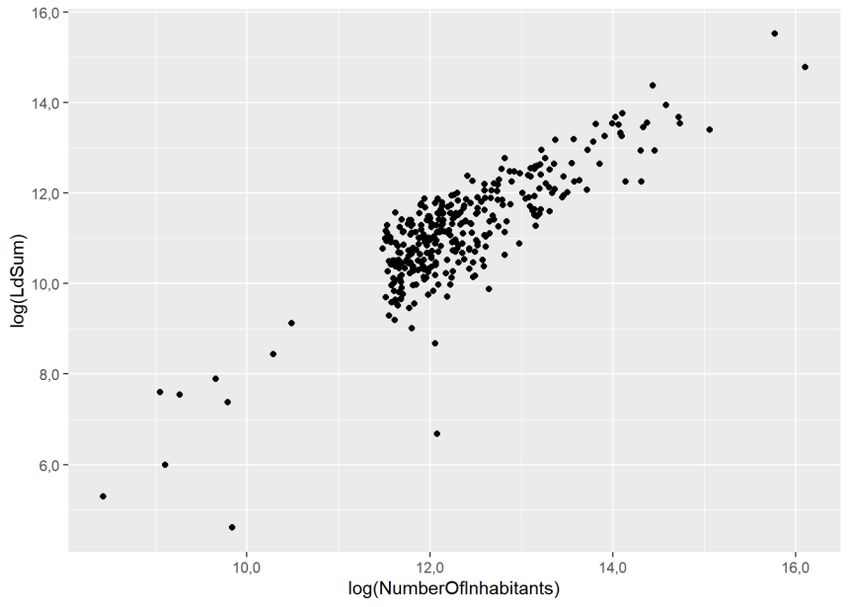
3.1.4 Visual inspection of the relationship between people exposed and number of
 inhabitants
The first step for conducting the regression is to look at the scatter plot between the two involved
variables: people exposed and the number of inhabitants (Figure 3.3). At first sight, it seems to fit a
perfect linear regression. However, given the skewed distribution of both variables, a log-log
transformation shows a better approximation to a normal distribution of both variables (Figure 3.4).
In that case, we will test the following models:
People_exposed = a + b*Number_inhabitants
People_exposed = a + b*Number_inhabitants + c*Number_inhabitants2
Log(People_exposed) = a + b*log(Number_inhabitants)
The second model corresponds to a polynomial regression of order 2, which is useful when there is a
small bending on the relationship between the two variables. Although it is not evident that it would
be useful in that case, we will include it as an illustration that it can be easily implemented and tested.
Zero values in the log transformation are problematic since log(0) is not a real number. Therefore, in
the case of zero values, we should add a small amount to all zeros: 0,1. This does not impact the total
number of people exposed while keeping the agglomeration in the regression analysis. This is relevant
for Lnight. As it is logical, no zero values have been observed in people exposed to Lden equal or greater
to 55 dB.

Figure 3.3: Scatterplot of the number of inhabitants and people exposed to noise from roads inside
 agglomerations (Lden equal or greater than 55 dB). N = 329 agglomerations

Eionet Report - ETC/ATNI 2021/6 15

Figure 3.4: Log-log transformation of the number of inhabitants and people exposed to noise from
 roads inside agglomerations (Lden equal or greater than 55 dB). N = 329 agglomerations

3.1.5 Data subsetting for regression analysis and validation
Data subsetting refers to divide the agglomerations where data has been reported into two groups:
one for estimating the regression parameters and the other one to validate the regression. Then, we
apply the regression model to the second subset, validation, which is independent of the data used to
estimate the model. Finally, the outcome can be compared with the original data.

The following requirements are needed for subsetting:
 • The minimum number of samples (agglomerations). The total number of (complete) data
 should follow the rule (Snee, 1977)
N > 2*(nr of independent parameters) +25
In our case, we only include one parameter resulting in 27 as the minimum number of agglomerations
required for a valid splitting.
 • As a general rule, data is split by a 70:30 ratio, being 70 for estimating the model and 30 for
 validation (Snee, 1977).
According to these rules, 226 agglomerations where data is reported -outliers excluded, have been
randomly divided as follows:
 • 226 agglomerations for estimating the regression model
 • 103 agglomerations for validation
Both subsets must follow the same distribution. The Kolmogorov–Smirnov test is a nonparametric test
of the equality of continuous one-dimensional probability distributions. The distribution of both
model and validation subset are depicted in Figure 3.5. In that case, the probability of the
Kolmogorov–Smirnov statistic is 0,47. Therefore, the null hypothesis that both data sets have the same
distribution is not rejected.
When the distributions significantly differ, a new random subset needs to be selected until the
condition of the same distribution is met.

Eionet Report - ETC/ATNI 2021/6 16

Figure 3.5: Distribution of two subsets of agglomerations: agglomerations used to estimate the
 regression model and agglomerations used for validation

3.1.6 Test models
The three models described in step 2 have been calculated on the subset of 226 agglomerations
selected for that purpose:
 • Model 1. Linear. People_exposed = a + b*Number_inhabitants
 • Model 2. Polynomic. People_exposed = a + b*Number_inhabitants + c*Number_inhabitants2
 • Model 3. Log-log. Log(People_exposed) = a + b*log(Number_inhabitants)
From the performance perspective, model 3 has the highest R2, followed by model 2, and model 1
(Table 3.3). The other statistics related to the model accuracy can only be compared between model
1 and model 2 since are scale-dependent -model 3 has been log-transformed. In all cases, the lower
of sigma, AIC, and BIC, the better. In that case, we see that model 2 has lower values than model 1.
Sigma measures the average error performed by the model in predicting the outcome (Table 3.3).
Therefore, sigma could be read as the error on estimating the people exposed to noise: there is a small
difference (about 6.300 people) between model 1 (229.022 people) and model 2 (222.724 people).
Finally, the F statistic p-value, which measures the statistical significance of the regression, is in line
with the previous statistics: model 3 is more significant than model 2, and model 2 is more than model
1 (Table 3.3).
In addition to the accuracy, diagnostic plots are relevant to identify the possible weakness of the
regression model. Figure 3.6 provides three of the most common diagnostic plots:
 • Residual versus fitted. This plot shows if residuals have non-linear patterns. All models have a
 certain deviation: model 1 and model 2 have a strong deviation on agglomerations with higher
 exposure (right side of the figure). Model 3 has a smaller deviation on both extremes. This
 indicates that other factors may be relevant to predict people exposed, and the number of
 inhabitants is only one factor -probably the main factor given the high level of prediction.
 • Normal Q-Q. This plot shows if residuals are normally distributed. Models 1 and 2 show that
 the extremes are problematic, while model 3 has a better fit to the line (normal distribution).
 • Residuals versus leverage. This plot helps us to find influential cases, if any. Agglomerations
 that are outside the dotted red lines (Cook’s distance) are influential in the model, i.e. these

Eionet Report - ETC/ATNI 2021/6 17

agglomerations have more weight on defining the model compared with the other
 agglomerations. Model 1 and Model 2 have three agglomerations with a strong impact on the
 model (three points outside the Cook’s distance represented by the dotted line). The log
 transformation in model 3 was effective in removing the strong influence of extreme values.
Details of the output are provided in Annex I.

Table 3.3: Statistics of the three tested regression models

 Model 1

 Model 2

 Model 3

Eionet Report - ETC/ATNI 2021/6 18

Figure 3.6: Diagnostic plots for the three regression models: residuals versus fitted (first row), normal Q-Q (second row), and residuals versus leverage (third
 row). Number are identifiers of agglomerations. Red line, trend of the plot. Dotted lines, Cook’s distance (0,5 and 1)
 Linear Polynomial Log-log

Eionet Report - ETC/ATNI 2021/6 19

3.1.7 Validation
In the previous step, we have seen that model 3 looked better because of higher R2 and better
performance on the diagnostics.
Table 3.4 and Figure 3.7 show the results of applying the 3 regression models to the subset selected
for validation (step 3). Model 1 and model 2 overestimate the population exposed, while model 3,
closer to the reported values, underestimate the population exposed. The % of the difference
between reported data and the estimates from the three models are very close, being model 3 being
the one with a lower percentage (5,9%). Also, the confidence interval for model 3 is lower. Therefore,
model 3 (log-log transformation) will be used to estimate the missing data. However, this result is data
specific and could not be generalised. Therefore, the most appropriate regression model should be
checked each time that the gap-filling is performed.

Table 3.4: Results of the validation of the three regression models. N = 103 agglomerations
 People % of Confidence
 exposed difference interval
 Reported 11.951.291
 Model 1 12.777.297 6,9 323.394
 Model 2 12.689.144 6,2 363.808
 Model 3 11.245.629 -5,9 279.311

Figure 3.7: Validation of the three regression models to estimate people exposed to noise from roads
 inside agglomerations (Lden equal or greater than 55 dB). Confidence interval (95%)
 provided for the regression models. n = 103 agglomerations

Eionet Report - ETC/ATNI 2021/6 20

3.1.8 Estimate values for missing data
Once the regression model has been selected, the following steps are taken:
 1. For each agglomeration where the data is missing, estimate the population exposed by
 applying the regression model. In that particular case, since we selected a log-log regression
 we have to transform back the estimated population exposed (anti log).
 2. Calculate the SE for each estimated value.

3.1.9 Calculate the total people exposed in Europe
 1. Sum all the estimated values
 2. We need to calculate the SE of the sum, which is obtained by quadrature of the individual SE
 3. Finally, calculate the confidence interval.

3.1.10 Estimate the people distributed by noise bands
Once the estimated total number of people exposed is calculated (previous step), we distribute the
population between the different noise bands.
 1. Based on the total number of people exposed per each agglomeration reported by Member
 States, we calculate the percentage that each noise band represent versus the total number
 of people exposed, for Lden and for Lnight, and then we derive the mean at European level.
 It needs to be taken into consideration that the percentage values have been obtained
 discarding the agglomerations providing 0 people exposed in all noise bands (Lden and Lnight, or
 Lden, or Lnight). Due to the rounding process, 0 could mean 0 to 49 people exposed; therefore,
 multiple combinations are possible with the same outcome of 0 people exposed.
 Consequently, an equal attribution of 20% of people exposed to each noise band only
 represents one of the multiple possible combinations. For that reason, agglomerations with 0
 people exposed are excluded.
 2. We apply the percentages to the agglomerations where we have estimated the total
 population, with the corresponding error of the estimate.
 3. Finally, we aggregate all the agglomerations at European level, with the corresponding
 estimation of the confidence interval.

Eionet Report - ETC/ATNI 2021/6 21

3.2 Gap filling method for railway noise, aircraft noise and industrial noise inside
 agglomerations
This section summarises the method applied to gap fill exposure information for railways noise,
aircraft noise and industrial noise inside agglomerations.
Figure 3.8 provides an overview of the process for estimating missing data, as Ramos (2019) described.
In each step, the decision tree uses the best approach according to the available ancillary data:
 • Use data from the previous reporting period if available.
 • When data from the previous reporting cycle is not available, data is estimated with the
 European average of the % of population exposed inside the agglomeration. In that case, no
 significant correlation was found between population exposed and other predictor
 parameters (e.g., the agglomeration population, area of the agglomeration); therefore, the
 European average is the best alternative (Fons et al., 2015).
 • Based on the total number of people exposed per each agglomeration reported by the
 Member States, we calculate the percentage that each noise band represent versus the total
 number of people exposed, for Lden and for Lnight. Then we derive the mean at European level.
 It needs to be taken into consideration that the percentage values have been obtained
 discarding the agglomerations providing 0 people exposed in all noise bands (Lden and Lnight, or
 Lden, or Lnight). Due to the rounding process, 0 includes figures ranging from 0 to 49 people
 exposed; therefore, multiple combinations are possible with the same outcome of 0 people
 exposed. Consequently, an equal attribution of 20% of people exposed to each noise band
 only represents one of the several possible combinations. For that reason, agglomerations
 with 0 people exposed are excluded.
 • We apply each noise band’s percentages to the agglomerations where we have estimated the
 total population, with the corresponding error of the estimate.
 • Finally, we aggregate all the agglomerations at European level, with the corresponding
 estimation of the confidence interval.
A more detailed explanation and the basis for the methodology applied in each step is provided in
Table 3.5.

The gap filling methodology also includes those few cases where data is missing for some noise bands.
Then, partial gap filling is conducted as follows:
 • Use data from the previous reporting period for the missing noise band(s).
 • If data from the previous reporting period is not available use the European average of % of
 the population exposed by noise band to estimate the missing data.
 • Table 3.2 provides an example of a partial gap filling when data from the previous period is
 not available.
Each step that involves the estimation of data, corresponding error is calculated. Finally, these errors
are propagated to the aggregated European figures as described in sections 3.1.9 and 3.1.10.

Eionet Report - ETC/ATNI 2021/6 22

Table 3.5: Methods used on the different steps of gap filling people exposed to noise from railways, airports and industry inside agglomerations. Numbers
 refer to the steps highlighted in Figure 3.1
 Step Method for gap filling Explanation Comment
 1 Exclude the agglomeration if An agglomeration reporting -1 for a source in the previous reporting cycle (tn-1), This step only applies if data is not reported, and “not
 it was reported as -1 (not meant that that source was not applicable according to the END specifications. applicable” is not explicitly mentioned at tn.
 applicable) at tn-1 Therefore, we retain the non-applicability at tn (Fons et al., 2016). Check done in
 previous gap-filled data (2016, 2017, 2018 and 2019) demonstrates that the
 assumption was correct in 90% of cases. Therefore, the potential
 underestimation of the European figure (data excluded) is more accurate than
 the overestimation, when all these agglomerations are gap filled.
 2 Exclude outliers from the Outliers from the change percentage between tn-1 and tn based on the Previous assessments have identified some extreme
 reported data to be used for interquartile range (IQR, the difference between 3rd and 1st quartile). The exact population changes exposed to noise between two reporting
 the European average (step threshold is ± 1,5 IQR. periods (Ramos, 2019). Therefore, the estimation of missing
 5) data in 2019 (Ramos, 2019), adopted a methodology to
 exclude outliers.
 3 Use the data delivered in the A comparative analysis described in Fons et al. (2017) concluded that this is the The method is constrained to the availability of the data on
 previous reporting period for method with the smaller error. the previous reporting cycle.
 the same agglomeration, if
 available.
 4 Estimate the total If the country reported the agglomeration's delineation, the population could be The reporting cycle of the Urban Atlas is always one year
 population from ancillary derived from Urban Atlas described in Fons et al. (2015). The average error of the later than the END.
 data. estimation based on Urban Atlas is 3%, ranging from 1 to 10%. If the delineation
 has not been reported, data from Eurostat can be used. The agglomeration
 population is the used in step 5.
 5 Estimate the population No significant correlation was found between population exposed and other
 exposed by multiplying the predictor parameters (e.g., the agglomeration population, area of the
 population of the agglomeration); therefore, the European average is the best alternative (Fons et
 agglomeration with the al, 2015).
 European average of the %
 of people exposed.
 6 Estimate the % of the Based on the total number of people exposed per each reported agglomeration, Initially, the % was calculated on a country basis when were
 population exposed per we calculate the percentage that each noise band represent versus the total enough agglomerations reported. Fons et al. (2017) concluded
 noise bands (%) from the number of people exposed, for Lden and for Lnight. Then we derive the mean at that using the country average has a similar error than the
 European average. European level. This approach is discussed in depth in Fons et al. (2015). European average. Therefore, the European average is used
 for simplicity.

Eionet Report - ETC/ATNI 2021/6 23

Figure 3.8: Overview of the process for estimating the population exposed to noise from rails, airports or industry inside agglomerations when data is not
 available. The methodology only applies to agglomerations that have to report according to END requirements. Numbers indicate specific
 methods for gap filling depending on available ancillary data -details are described in Table 3.4. Source: updated from Ramos (2019)

Eionet Report - ETC/ATNI 2021/6 24

4 END major roads and major railways exposure data outside
 agglomerations: gap filling

4.1 Gap filling method
This method is based on the working paper establishing a methodological proposal to interpolate a
complete coverage on noise exposure at EU level (ETC/ACM, 2015).
Figure 4.1 provides an overview of the process for estimating missing data, as Ramos (2019) described.
In each step, the decision tree uses the best approach according to the available ancillary data:
 • Partial gap filling if reported data is not complete. Data completeness can only be evaluated
 if exposure has been delivered by the road and rail segments. Then network segments are
 linked to DF1_5 dataflow to match segments to be reported with the actual data reported.
 Missing segments are gap filled with the regression between people exposed and the length
 of the transport network (the procedures is the same as described for roads inside
 agglomerations. It should be noted that the length of the transport network also includes
 major source inside agglomerations. However, the data reported on people exposed refers
 only to people outside agglomerations. When the exposure information has been delivered
 as one single value for the entire network, the codes are supplied as -1 or -2 or the codes
 between dataflows (DF1_5 and DF4_8) do not match, then the comparison of the code is not
 possible, and the dataset is assumed as complete.
 • If data is not reported, use data from the previous reporting period if available and complete
 (same procedure as explained in the above bullet point to evaluate completeness).
 • When data from the previous reporting cycle is not available or not complete, the regression
 between the number of people exposed and the transport network's length has been
 calculated. Then the regression has been applied to estimate missing data. In that case,
 complete gap filling is applied, i.e. even if some data (incomplete) is available from the
 previous period, the regression is applied to the full extent of the transport network. It should
 be noted that the length of the transport network also includes major source inside
 agglomerations. However, the data reported on people exposed refers only to people outside
 agglomerations.
 • Once the total number of people exposed is estimated, we distribute the total population
 exposed to the different noise bands based on the European average of the population
 exposed by noise bands. The European average is calculated with all the available data, even
 if it is incomplete for a certain region of the country. The European average discards the
 countries or regions providing 0 people exposed in all noise bands. Due to the rounding
 process, 0 could mean 0 to 49 people exposed. Therefore attributing 20% to each noise band
 would not be accurate since other options would also be feasible.

Eionet Report - ETC/ATNI 2021/6 25

Table 4.1: Methods used on the different steps of gap filling people exposed to noise from roads
 inside agglomerations. Numbers refer to the steps highlighted in Figure 3.1

 .Step Method for gap filling Explanation Comment
 1 Use the data delivered A comparative analysis described in The method is constrained to the
 in the previous Fons et al. (2017) concluded that availability of the data on the
 reporting period, if this is the method with the smaller previous reporting cycle, and the
 available. error. data is complete.
 2 When the data is not The methodology for partial gap The current report provides a
 complete for a certain filling is described in Fons et al. detailed description of the metrics
 country, estimate the (2015). to evaluate the best regression
 missing data with the The regression and correlation model, including estimating the
 regression between analysis between population error and confidence interval in
 people exposed and the exposed and potential predictors the final aggregation of data (EU
 length of the transport (country area, length of transport figures). There is no a priory
 network. network) is documented in Fons et regression model to be applied
 al. (2015). Later on, Fons et al. each time that the gap filling is
 2017) demonstrated that, if developed. The regression model
 available, using data from the needs to be checked each time
 previous reporting period (step 1) since the relationship is strongly
 is more accurate than the dependent on the data included
 regression approach. for the regression. The approach
 described in section 3.1 is also
 valid here.
 3 Estimate the population The regression and correlation The current report provides a
 exposed from the analysis between population detailed description of the metrics
 regression between exposed and potential predictors to evaluate the best regression
 population exposed and (country area, length of transport model, including estimating the
 km of road or rail. network) is documented in Fons et error and confidence interval in
 al. (2015). Later on, Fons et al. the final aggregation of data (EU
 2017) demonstrated that, if figures). There is no a priory
 available, using data from the regression model to be applied
 previous reporting period (step 1) each time that the gap filling is
 is more accurate than the developed. The regression model
 regression approach. needs to be checked each time
 since the relationship is strongly
 dependent on the data included
 for the regression. The approach
 described in section 3.1 is also
 valid here.
 4 Estimate the % of the Based on the total number of
 population exposed per people exposed, we calculate the
 noise bands (%) from percentage that each noise band
 the European average represent versus the total number
 of people exposed, for Lden and for
 Lnight, and then we derive the mean
 at European level. This approach is
 discussed in depth in Fons et al.
 (2015).

Eionet Report - ETC/ATNI 2021/6 26

Figure 4.1: Overview of the process for estimating the population exposed to noise from major roads and major rails when data is not available. The
 methodology only applies to countries that have to report according to END requirements. Numbers indicate specific methods for gap filling
 depending on available ancillary data -details are described in Table 4.1. Dotted lines: data partially reported, and data partially gap filled.
 Source: updated from Ramos (2019)

Eionet Report - ETC/ATNI 2021/6 27

5 END Major airport exposure outside agglomerations: gap filling

5.1 Overview
The current methodology to estimate missing data on the population exposed to major airports
outside agglomerations is presented in Figure 5.1 (Ramos, 2019). In this case, we start with the
calculation of the average relative change of population exposed between the current reporting period
(t2) and previous cycle (t1) as described in Jones (2013):
 2 − 1
 ∑ =1 ( )
 1
 =
 
Where n is the number of major airports with reported data for the period t1 and t2, being t2 the current
reporting cycle, and i is the ith major airport where data is available.
In practical terms this relative difference can be expressed as ratio and directly applied to those major
airports where data for the current reporting period is missing, but available for the previous period:
 2
 ∑ =1 ( )
 1
 =
 
Then, this ratio It should be noted that the use of the ratio of change could be extended back up to
two reporting cycles. For example, in the case that data for a certain major airport is only available for
2007, then we calculate the ratio of change for the period 2007 – 2017 and apply this ratio to the data
of 2007.
In this case outliers have also to be excluded from the calculation as explained in the case of roads
inside agglomerations.
The use of the relative difference is based on the fact that it provides better estimates than any other
predictor, e.g. number of annual flights (Fons et al., 2016). The low correlation between people
exposed and the number of flights is explained by the fact that exposure to aircraft noise is strongly
dependent on local conditions, including specific operational measures (take-off and landing routes,
time of the day,…), meteorological conditions, or land use planning. However, the current approach
has its limitations since it assumes a homogenous change ratio in all agglomerations. Figure 5.2 and
Figure 5.3 illustrate the distribution of the relative difference between 2012 and 2017. The value
ranges from -1 (100% decrease on exposure) to 1,5 (150% increase of population exposed). About 9
out of 40 major airports are outliers (23%).

Eionet Report - ETC/ATNI 2021/6 28

Figure 5.1: Overview of the workflow for estimating the population exposed to major airports outside
 agglomerations when data is not available. Source: Ramos (2019)

 Has the major airport Use DF4_8 2017 data for major
 X DF4_8 2017 data?
 Yes airport X

 No

 Has the major airport Estimate people exposed to Lden>55 dB or Lnight>50db 2012 applying
 Yes multiplication factor 2017-2012
 X DF4 2012 data?

 Distribute the estimated value of
 No people exposed to Lden>55dB or
 Lnight>50db following the EU
 distribution

 Has the major airport
 X DF4 2007 data?
 No Excluded

 Yes

 Distribute the estimated value of
 Estimate people exposed to Lden>55 dB or Lnight>50db 2012 applying people exposed to Lden>55dB or
 multiplication factor 2007-2017 Lnight>50db following the EU
 distribution

Eionet Report - ETC/ATNI 2021/6 3

Figure 5.2: Box plot of the relative change of population exposed to noise from major airports
 between 2012 and 2017 (Lden ≥ 55 dB). Outliers are indicated in red. The lower and higher
 limits of the box correspond to the 1st and 3rd quartile, respectively. The horizontal line
 inside the box is the median

Figure 5.3: Distribution of the population relative change exposed to noise from major airports
 between 2012 and 2017 (Lden ≥ 55 dB). Outliers in green

 Lden Relative change (2017 – 2012)

Eionet Report - ETC/ATNI 2021/6 4

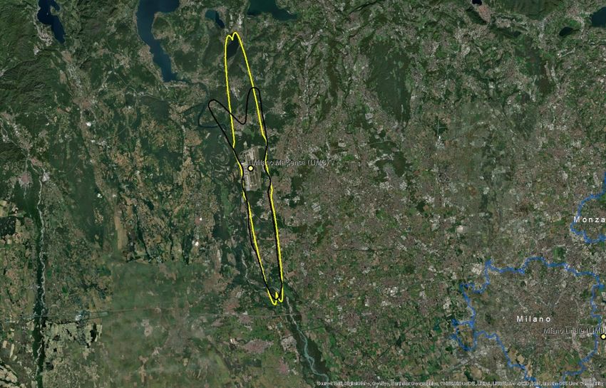
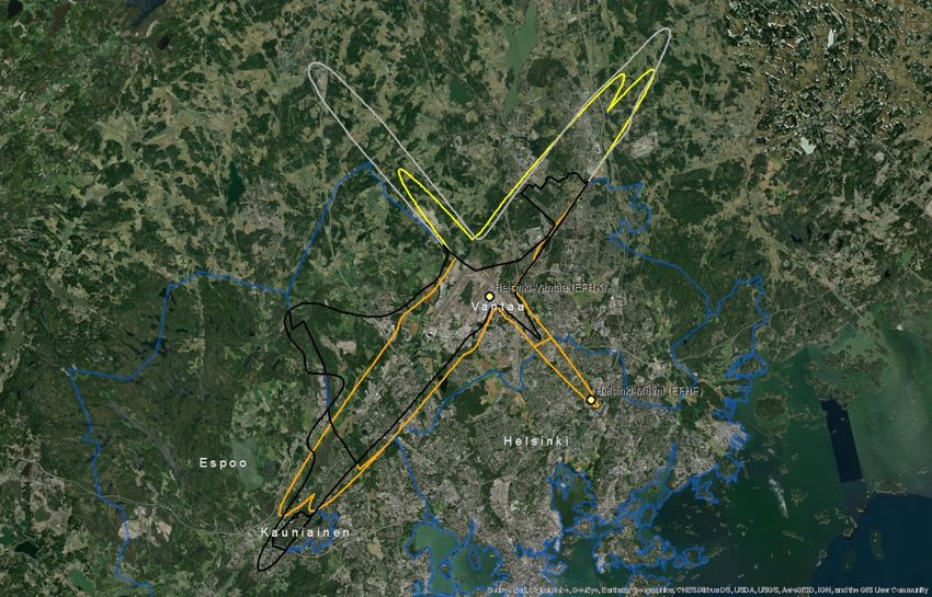
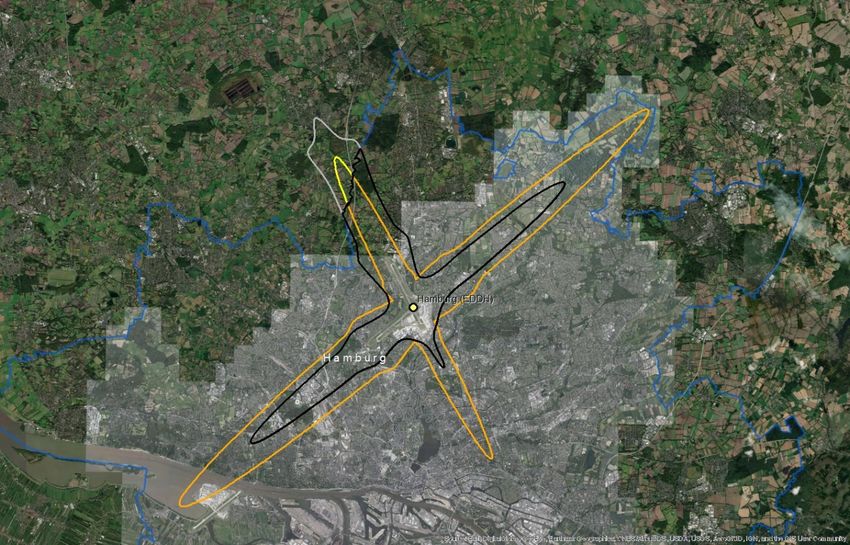
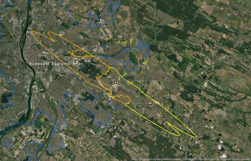
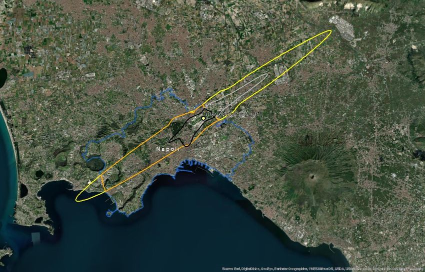
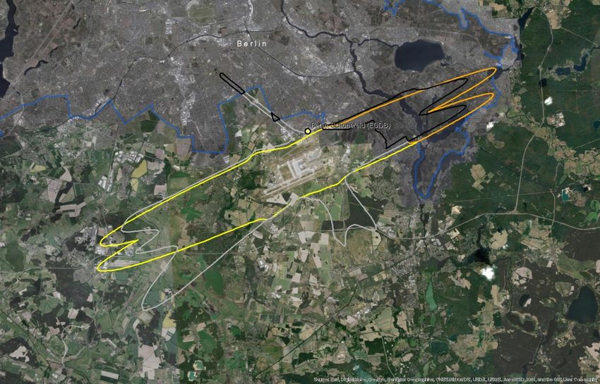
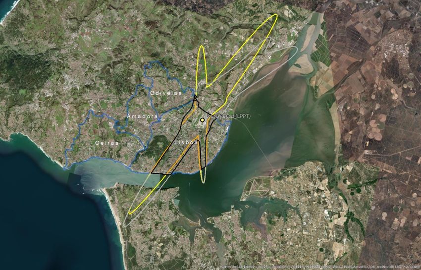
Since the outliers are equally distributed around the mean, there is no major impact on the average
ratio if we include them in the calculation (Table 5.1). However, the standard error decreases by 40%
when outliers are excluded. Moreover, if outliers are not excluded, the estimated confidence interval
of the change ratio ranges from a small decrease (-0,03) to 0,18 increase because the standard error
(0,10) is higher than the average (0,08), as presented in Table 5.1.

Table 5.1: Mean, upper and lower boundaries of the confidence interval (95%), and standard error
 (SE) of the change of population exposed to noise from major airports between 2012 and
 2017 (Lden ≥ 55 dB). Data is presented for the complete set of available major airports and
 for the subset without outliers. N is the number of major airports
 Lower Average Upper boundary SE n
 boundary
 With outliers -0,03 0,08 0,18 0,10 40
 Without outliers 0,03 0,08 0,14 0,06 31

Given all these uncertainties, the current report provides an alternative method and test its suitability
and potentially higher performance. Our hypothesis is that delineating an approximated noise contour
band in those major airports that have not reported data will better estimate the population exposed
than the current method. We assume that with this approach, we better capture local conditions with
a reasonable effort of computation.
The methodology has been tested in 10 airports where all the information has been reported (Table
5.2).

Table 5.2: Airports selected to test the proposed methodology. Airports with the same arrangement
 of runaways have the same colour
 Airport ICAO code Annual traffic Runaways

 Berlin-Tegel EDDT 182200 2 runways (side-by-side)
 Berlin-Schönefeld EDDB 70324 2 parallel runways
 Copenhagen EKCH 251799 3 runways cross model
 Hamburg EDDH 153876 2 runways cross model
 Helsinki-Vantaa EFHK 168704 3 runways, 2 parallel, one crossing
 (almost perpendicular)
 Lisbon LPPT 159795 2 runways cross diagonal disposal (45
 degrees)
 Milano-Malpensa LIMC 166509 2 parallel runways

 Napoli LIRN 64712 1 runway
 Wien LOWW 226811 2 runways diagonal disposal
 Budapest Ferihegy LHBP 96705 2 runways diagonal disposal

Eionet Report - ETC/ATNI 2021/6 5

5.2 A methodology based on estimating the noise contour around runaways

5.2.1 Overview
The methodology to estimate the population exposed to major airports (Lden) is synthesised in Table
5.3. The method for Lnight would be similar.

As can be seen, the methodology has two major elements of uncertainty:
 • Delineation of the noise contour around the major airports. These contours depend on several
 factors: number and length of runaways, local regulations, meteorological conditions, or
 orography, just to name some of them.
 • Assuming that all the population living inside the contour is exposed to noise. Therefore,
 existing measures like building insulation are not considered since it is not feasible to introduce
 this component at European scale.

Table 5.3: Methodology to estimate population exposed to major airports (inside and outside
 agglomerations)
 Steps Output Comments
 1. Delineation of the noise
 contour for Lden 55dB (lower Noise contour for Lden
 boundary) 55dB (lower boundary)

 From satellite imagery draw a simple line
 a. Identify runaway(s) representing the full length of each
 runaway
 b. Delineation of the
 contour for Lden 55dB Delineation of the contour based on a
 around runaways certain buffer around the runaways

 In case of the presence
 2. Cross the contour of Lden 55dB of one or more This step is needed to differentiate the
 with the delineation of the agglomerations: people exposed outside and inside the
 agglomeration contour outside and agglomeration (if the contour intersects
 contour inside with one or more agglomerations)
 agglomerations(s)
 Cross the areas of the previous step with
 3. Calculate the population inside Distribution of the the population grid. The obtained value
 the noise contour (inside and peoples exposed by will be an estimate of the population
 outside the agglomeration) noise bands exposed to a major airport (inside and
 outside agglomerations).
 4. Distribute the total population Apply the European average of % of
 exposed to major airport by population exposed distributed by noise
 noise bands bands.

Eionet Report - ETC/ATNI 2021/6 6

5.2.2 Data requirements
The following data has been used to test the methodology:
 • Reference image for runaways: Google Maps
 • Delineation of agglomerations as provided by the information reported by countries according
 to END specifications
 • Noise contour bands reported by countries
 • Population. Outside agglomerations, GEOSTAT population at 1 km grid(2)

5.2.3 Delineation of the runaways and noise contours
The most critical issue is the delineation of the noise contour. During the testing phase, it was taken
into consideration the use of wind maps and its monthly/year direction means as usually aircraft
depart and arrive counter wind. As well ATS routes, traffic maps and the use of waypoints and fixes to
determine routes were analysed to determine the most common path of planes in each airport, but
unfortunately, no relevant data was found. Many airports implement noise mitigation techniques
(noise abatement procedures), that increases the uncertainty when creating a common delineation
noise model, including the following:
 • Defining noise abatement procedures that avoid residential areas as far as possible and avoid
 over-flying sensitive sites such as hospitals and schools
 • Using continuous descent approaches and departure noise abatement techniques
 • Ensuring that the optimum runway(s) and routes are used as far as conditions allow
 • Avoiding unnecessary use of auxiliary power units by aircraft on-stand
 • Building barriers and engine test-pens to contain and deflect noise
 • Towing aircraft instead of using jet engines to taxi
 • Limiting night operations
 • Limiting the number of operations or the extent of a critical noise contour
 • Providing noise insulation for the most severely affected houses
 • Applying different operational charges based on the noisiness of the aircraft
 • Monitoring individual noise levels and track keeping and penalising any breach
However, since this approach is quite effort consuming, it was decided to take one airport as a model
and replicate the noise contour on the airports without data, adapted to the length of the runaways.
For the one runway setup airports, the replication of the Tegel delineation is enough to have a strong
approach close to the reality on the gap filled airports. When talking about two or three-runway setup,
the complexity is higher. Despite that, taking into account what has been reported on contour maps,
Table 5.4 shows the type of artificial delineations created to calculate the population exposed and gap-
fill missing data:
In relation to the generated contour maps for gap filling, the best way to replicate the possible track
of the aircraft is to look at what is happening in the airports; there is information reported. Depending
on many factors such as frequent wind flows, orography, local regulations, etc, an aircraft creates one
type of noise path or another. On perfect conditions, the most common is that the plane creates a

(2) https://ec.europa.eu/eurostat/web/gisco/geodata/reference-data/population-distribution-demography/geostat

Eionet Report - ETC/ATNI 2021/6 7