Filtering method based on cluster analysis to avoid salinity drifts and recover Argo data in less time
←
→
Page content transcription
If your browser does not render page correctly, please read the page content below
Ocean Sci., 17, 1273–1284, 2021
https://doi.org/10.5194/os-17-1273-2021
© Author(s) 2021. This work is distributed under
the Creative Commons Attribution 4.0 License.

Filtering method based on cluster analysis to avoid salinity drifts
and recover Argo data in less time
Emmanuel Romero1 , Leonardo Tenorio-Fernandez2 , Iliana Castro1 , and Marco Castro1
1 Tecnológico   Nacional de México/Instituto Tecnológico de La Paz, La Paz, México
2 CONACyT-Instituto    Politécnico Nacional-Centro Interdisciplinario de Ciencias Marinas, La Paz, México

Correspondence: Leonardo Tenorio-Fernandez (ltenoriof@ipn.mx)

Received: 11 March 2021 – Discussion started: 6 April 2021
Revised: 17 July 2021 – Accepted: 27 July 2021 – Published: 17 September 2021

Abstract. Currently there is a huge amount of freely avail-           1   Introduction
able hydrographic data, and it is increasingly important to
have easy access to it and to be provided with as much in-            Autonomous oceanographic instruments have become very
formation as possible. Argo is a global collection of around          important tools in observational oceanography. Hydro-
4000 active autonomous hydrographic profilers. Argo data go           graphic autonomous profilers (HAPs) are tools that reduce
through two quality processes, real time and delayed mode.            the costs of in situ oceanographic observations, obtaining a
This work shows a methodology to filter profiles within a             large number of hydrographic profiles in time and space, at
given polygon using the odd–even algorithm; this allows               a lower cost compared to those carried out on oceanographic
analysis of a study area, regardless of size, shape or location.      cruises. An example of these HAPs is those belonging to the
The aim is to offer two filtering methods and to discard only         Argo program, in which each measured profile is processed
the real-time quality control data that present salinity drifts.      by its Data Assembly Center (DAC) in a quality control sys-
This takes advantage of the largest possible amount of valid          tem, before being published (Argo Data Management Team,
data within a given polygon. In the study area selected as an         2019).
example, it was possible to recover around 80 % in the case              HAPs have the ability to continuously measure hydro-
of the first filter that uses cluster analysis and 30 % in the case   graphic parameters in the water column. Since the beginning
of the second, which discards profilers with salinity drifts, of      of the program and up to the present, there are data records
the total real-time quality control data that are usually dis-        collected from around 15 300 core HAPs and around 1300
carded by the users due to problems such as salinity drifts.          biogeochemical HAPs belonging to the global Argo group in
This allows users to use any of the filters or a combination of       the world oceans, which have measured temperature, salinity
both to have a greater amount of data within the study area of        and biogeochemical parameters in most cases from 2000 m
their interest in a matter of minutes, rather than waiting for        depth to the sea surface or vice versa, from which around
the delayed-mode quality control that takes up to 12 months           4000 are currently active (Argo, 2020a). However, around
to be completed. This methodology has been tested for its             75 % of the total profiles have completed the quality control
replicability in five selected areas around the world and has         process, and therefore it is considered that the rest may or
obtained good results.                                                may not be of such good quality. In areas with a low concen-
                                                                      tration of profiles, this percentage is more significant, and it
                                                                      is important to obtain as much data as possible to support
                                                                      scientific research.

Published by Copernicus Publications on behalf of the European Geosciences Union.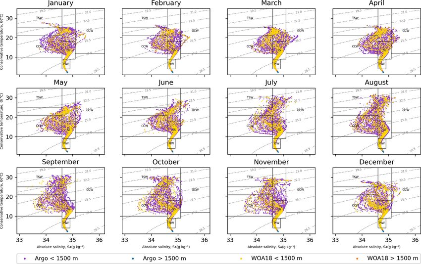
1274                                                                E. Romero et al.: Filtering method to avoid salinity drifts

   The data of each HAP have to be validated and processed
by a quality control system, before being used or published.
The Argo quality control system consists of two stages, real-
time quality control (RTQC) and delayed-mode quality con-
trol (DMQC). The tests performed by the RTQC are auto-
mated and limited, due to the requirement to be available
within the first 24 h after transmission. These data are free of
serious errors in each of their variables (e.g. impossible data
in dates and coordinates) and must be within the global and
regional ranges. In the case of having adjusted parameters
available, these are placed in the same variables, but named
with the suffix “_ADJUSTED”; in this way the data are pre-
served without adjustments in the variables without this suf-
fix. The second quality control process is the DMQC. The
data adjusted by this quality control replace the data adjusted     Figure 1. Study area. The upper right corner shows the location of
by the RTQC. Since, during this process, the data are sub-          the study area composed of parts of the California Current System,
jected to detailed scrutiny by oceanographic experts, DMQC          the Gulf of California, the transition area and the tropical Pacific off
data can take a year to be published (Wong et al., 2021). Nor-      central Mexico (TPCM), shown in the foreground.
mally, due to the problems presented by the RTQC data, such
as the salinity drifts presented in this work, users of Argo pro-
gram data are advised to only use DMQC data for scientific
analysis, or to perform it by themselves; this quality control      the California Current, the Gulf of California current and to
is explained in the manuals, and for this reason many users         the north the Mexican Coastal Current (Lavín and Marinone,
decide not to use the RTQC data.                                    2003; Lavín et al., 2009; Godínez et al., 2010; Portela et al.,
   The objective of this work is to present a methodology           2016). These interactions produce intense mesoscale activ-
based on cluster analysis to admit the data in RQTC that con-       ity and a high complexity in the circulation (Kessler, 2006).
forms to the same hydrography patterns as the DMQC data             Two mesoscale structures such as cyclonic and anticyclonic
and thus increase the amount of data available for scientific       eddies interact and play an important role in circulation (Za-
research, avoiding the complete discard of the RTQC data.           mudio et al., 2001, 2007; Lavín et al., 2006; Pantoja et al.,
To carry out this methodology, first, the data must be delim-       2012). As well as this, this area is part of the minimum oxy-
ited by a polygon, the one that represents the study area of        gen zone (Fiedler and Talley, 2006; Stramma et al., 2008).
interest. Using a point-in-polygon (PIP) algorithm the pro-         The study area encompasses parts of the California Current
files that were measured within the study area of interest are      System, the Gulf of California, the transition area and the
determined. In addition, a web application was developed to         tropical Pacific off central Mexico (Portela et al., 2016); here-
show the results of the application of this methodology and         inafter this study area will be named TPCM.
the usefulness that it can have if it were integrated into the         One of the great benefits of using a PIP algorithm to fil-
HTTP data access platforms, such as statistics and graphs of        ter locations is that it can be used with data from other geo-
study areas defined by the user.                                    referenced databases. To demonstrate this, tests were carried
                                                                    out with the World Ocean Atlas 2018 (WOA18) database,
                                                                    which provides quality-controlled data to calculate the cli-
2   Data collection and methods                                     matology of temperature, salinity, dissolved oxygen and dis-
                                                                    solved inorganic nutrients derived from profiling floats, OSD
To achieve the objectives of this research in any study area        (ocean station data), CTD (conductivity, temperature and
given by a polygon, irregular or not, and since the selection       depth) and many other contents in the NCEI World Ocean
of the data can be of interest both at a global and regional        Database 2018 (WOD18). The monthly data of temperature
level, the geographical coordinates of the profiles stored on       (Locarnini et al., 2018) and salinity (Zweng et al., 2018) of
the servers of Argo were used as points for the PIP problem         the statistical mean of each quarter degree (1/4◦ ) from 2005
and thus determine if they were measured within the study           to 2017 were downloaded, and the PIP algorithm described in
area. To solve it, the even–odd algorithm (Foley and Hughes,        this work was applied to the polygon that delimits the TPCM.
1990) was used, and once the profiles within the polygon are        Conversions from in situ temperature to conservative temper-
obtained, the profile data are downloaded.                          ature and practical salinity to absolute salinity were carried
   For the purposes of testing the methods of this work, a          out according to the Thermodynamic Equation of SeaWater
study area was selected (Fig. 1), which is located between 25       2010 (TEOS-10). The monthly T –S (temperature and salin-
and 19◦ N and 113 and 105◦ W. In this area it is known that         ity) diagrams of the WOA18 data and the Argo DMQC data
there are current interactions between the tropical branch of       were compared to corroborate that they are located in the

Ocean Sci., 17, 1273–1284, 2021                                                           https://doi.org/10.5194/os-17-1273-2021
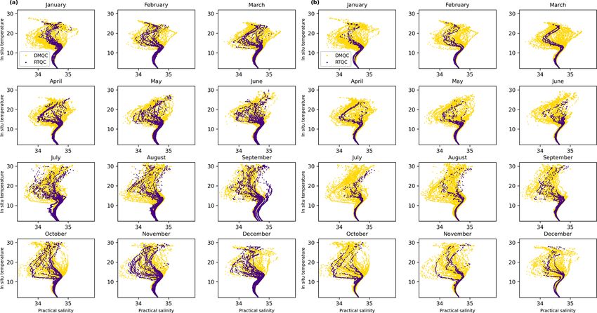
E. Romero et al.: Filtering method to avoid salinity drifts                                                                   1275

same water masses and to review the quality of the DMQC
data in the area.
   The data measured within the TPCM were statistically an-
alyzed, and it was found that there are few profiles within
the area and that around only 30 % of the total data have
been evaluated by the RTQC. The Argo manual (Argo Data
Management Team, 2019) indicates that the quality control
flags establish how good or bad the data are, with 1 being
good data and, as the value increases, the quality deterio-
rates. These flags are determined in the RTQC, and when
the DMQC arrives it creates flags for the adjusted data. In
the event that data have been adjusted in the RTQC, they are
replaced, because during the RTQC only gross errors can be
identified by the automated procedures, and to detect more
subtle issues with sensor drift these can only be carried out in
DMQC (Wong et al., 2021). Tests were performed by graph-
ing the T –S diagrams using these flags and adding the den-
sity isoline and the water masses according to Portela et al.
(2016). The RTQC data of all the flags were used, and all of
them showed salinity drifts, including the marked data with
flag 1 as seen in supplementary material A.1 (Romero et al.,       rithm separates these data by month in an array and iterates
2021b), so it is not feasible to use these indicators to filter    them. Within each iteration, it calculates the salinity mid-
the data in RTQC. To increase the amount of available data,        range of each quality control and divides the data measured
cluster analysis was applied to the data, since two groups of      at depths greater than that specified by the user, 1500 m by
data can be visually located in the T –S diagrams: those that      default, into two groups (using the mid-ranges as the starting
form the same patterns as those of the DMQC and those that         position of the centroids), up to a maximum of 10 iterations,
do not. This analysis groups a set of objects in such a way        each time verifying if there are DMQC data in both groups.
that the characteristics of the objects of the same group are      If so, the algorithm stops and returns the data without group-
more similar to each other than to the other groups (Everitt       ing them; on the contrary, if only a group contains the data
et al., 2011). In this case, the aim is to separate the RTQC       in DMQC, it associates the data of that group with the data
data into groups, a group that contains data with character-       at depths less than that specified by the user, taking into con-
istics similar to DMQC data and other groups with salinity         sideration the month, the profiler code and the profile num-
drift problems.                                                    ber, and replaces the group data with the associated data. The
   To perform the cluster analysis, the unsupervised k-means       mid-ranges are used as the initial position of the centroids to
classification algorithm was chosen, which groups the data         prevent them from being generated randomly. The procedure
into k groups, minimizing the distance between the data and        described above is the first filter of the RTQC data; in each
the centroid of its group (Hartigan and Wong, 1979). The al-       iteration the algorithm discarded the groups that presented
gorithm starts by setting the k centroids in the data space,       salinity drifts and kept only the group where the DMQC data
regardless of where the data were obtained, and assigning          were found, and thus, when the execution of the algorithm
the data to their closest centroid. Then, it updates the posi-     ends, RTQC data within the group with DMQC data are con-
tion of the centroid of each group, calculating the position       sidered to contain no salinity drifts. To increase the reliabil-
of the average of the data belonging to each group, and the        ity of the filtering, a second filter was created. In the second
data are reassigned to their closest centroid. This process is     filter, the algorithm stores in memory the profilers that pre-
repeated until the centroids do not change position. An al-        sented salinity drifts during the execution of the Algorithm 1.
gorithm based on distances was selected because it seeks to        Thus, the second filter not only discards the profiles with drift
obtain only the RTQC data closest to the DMQC data.                problems, it also directly discards all the profiles of the pro-
   Since it is necessary to indicate the number of k centroids     filers that they have at least one profile with salinity drifts.
when we use k-means, a manual enumeration of the groups                A library was developed that contains all the procedures
to be searched is required. To automate this process and avoid     described in this work. Using it, as an extra example, five
the user having to indicate the exact number of centroids          study areas were delimited with different extensions, loca-
needed to retrieve RTQC data for each month and for each           tions, profile densities and hydrographic characteristics. The
study area chosen, Algorithm 1 was programmed.                     first area was the Alboran Sea, which was selected because
   Algorithm 1 receives the adjusted data from the DMQC            the data were measured in shallow water (0 to 1200 m). The
and the RTQC; in the case of profiles that have not been ad-       Antarctic area was selected because of its high latitude (cold
justed, the data are received without adjustment. The algo-        water). The third area was the Bermuda Triangle, which was

https://doi.org/10.5194/os-17-1273-2021                                                        Ocean Sci., 17, 1273–1284, 2021
1276 E. Romero et al.: Filtering method to avoid salinity drifts
selected because it is located in the Atlantic transition be- On the contrary, the data in RTQC with the best quality
tween the tropical and subtropical area. The fourth is the flag present drifts in salinity. The RTQC and DMQC data
tropical zone of the Pacific that surrounds an archipelago of were plotted in the T –S diagrams together per month of the
the central Pacific, and the last one is in the tropical sea of TPCM, and some of the data in RTQC were the cause of
Indonesia. All data from these areas were downloaded from salinity drifts in almost all the months (Fig. 3).
the snapshot of December 2020 (Argo, 2020b) and evaluated In Fig. 3 it is clear that the salinity drifts in the RTQC data
by Algorithm 1. are important; however, it is also shown that certain data fol-
To test the above methods in a more extensive and irreg- low the structure (shape) of the DMQC data. To avoid dis-
ular polygon area, a web application was developed. The carding all RTQC data, the use of cluster analysis is pro-
study area for this web application was delimited using the posed. By applying cluster analysis to all data in RTQC with
Exclusive Economic Zone (EEZ) of Mexico as an example, the k-means algorithm and with different values in k, the re-
and the geographical location of the profiles from around sulting groups mix data that show salinity drifts with data
the world are filtered by the PIP algorithm, to automati- that follow the same patterns as the DMQC data at 1500 m.
cally download the data every 24 h within this irregular poly- This is because, at depths less than 1500 m, salinity data are
gon through the IFREMER synchronization service (avail- more dispersed than at greater depths.
able at http://www.argodatamgt.org/Access-to-data, last ac- Taking into consideration that at depths greater than
cess: November 2019). 1500 m, the variations in salinity and temperatures are im-
Every time that new data from HAPs are downloaded, they perceptible in this study area, the cluster analysis was per-
go through a processing phase, in which they are cleaned and formed with the salinity data measured at depths greater than
transformed to be integrated into the web application. For ex- 1500 m. The resulting groups are shown in Fig. 4a and b,
ample, the variables of temperature and salinity are converted and in the figure it can be observed that one of the result-
to conservative temperature and absolute salinity, as defined ing groups contains the data that follow the same patterns as
by TEOS-10; the current description of the properties of sea- the DMQC data, and the rest of the groups contain data with
water defines it. Afterwards, graphs and useful files are gen- salinity drifts. Therefore the next step was to associate the
erated to show information about the HAPs and their profile data of these groups with the rest of the data, taking into con-
data. sideration the profiler code and the profile number and thus
The web application was developed on a satellite map, to obtaining complete groups (Fig. 4c and d).
which tools were added for data management and visualiza- Figure 4 shows how the groups are separated with the
tion, such as drawing irregular polygons to define study ar- chosen algorithm. In the months of January and November,
eas within the main polygon, filtering data to display statis- DMQC data are displayed as yellow dots and the orange
tical and graphical data according to the selected filter and groups contain the RTQC data that follow the patterns of the
trajectory tracing, among others. Also, RTQC data filtering data in DMQC. The blue, green and red groups contain the
was implemented in the web application. The same irregular data showing salinity drifts.
polygons with which statistical data are obtained can be used To avoid indicating the number of k centroids manually,
to indicate a study area in which as much data as possible is Algorithm 1 was developed. Figure 5 shows the first three it-
obtained without salinity drifts. erations of the month of November as an example. In Fig. 5a
and b blue data represent the group that contains DMQC data
and the orange color group represents the group of the RTCQ
3 Results data. The data contained in the orange groups are discarded
by the algorithm. Figure 5c is the third iteration, and both
The data used to obtain the following results were down- groups contain data in DMQC, because the data are so close
loaded from the Coriolis GDAC FTP server in 2019 and to each other that the k-means algorithm (which is based on
the “Profile directory file of the Argo Global Data Assem- distances to separate the groups) divides the DMQC data into
bly Center” file was used as input for the chosen PIP algo- two different groups, so that in this iteration the algorithm
rithm, which filtered the measured profiles inside the poly- stops.
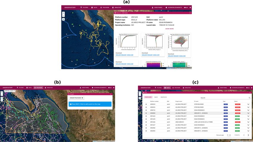
gon correctly. Figure 2 shows the result of the T –S diagram The results of the first filtering of the proposed algorithm
comparison between the DMQC data and the WOA18 data. are shown in Fig. 6a. The filtered data from the RTQC show
The DMQC and WOA18 data are located in the same wa- the same patterns as the DMQC data, except for the months
ter masses, and the data are spliced at depths greater than of July, August and September. In July and August, the salin-
1500 m, which validates that the DMQC data follow the same ity drifts are found at depths less than 1500 m, while in
patterns as the data from other international databases. Ac- September, the drifts present values very close to the DMQC
cording to Portela et al. (2016), this region is made up of data and this prevents the algorithm from being able to sep-
the California Current Water (CCW), Tropical Surface Water arate them. This filter allows a greater amount of admitted
(TSW), Gulf of California Water (GCW), Subtropical Sub- RTQC data to be obtained, but as seen in the figure, it still
surface (SS) and the Pacific Intermediate Water (PIW). shows salinity drifts in some cases. For this reason, the sec-
Ocean Sci., 17, 1273–1284, 2021 https://doi.org/10.5194/os-17-1273-2021
E. Romero et al.: Filtering method to avoid salinity drifts                                                                   1277

Figure 2. Monthly comparison of T –S diagrams of data from DMQC and WOA18. The black boxes delimit the limits of the water masses
in the region and the gray isolines the density (kg m−3 ).

ond filter was incorporated. Figure 6b shows the results of         filter if the user wishes to use only the most reliable data.
it, since it considers those profilers that have presented salin-   Also, the possibility of using a combination of both filters is
ity drifts and removes their profiles completely, a significant     not ruled out – if the user uses the months of the first filter
reduction in admitted data from the RTQC is observed, but           that no longer present salinity drifts and uses the data of the
these no longer show salinity drifts.                               second filter in which they present drifts, the largest possible
    Table 1 shows the total measurements (Meas.) made in the        amount of admissible data would be used in any study area.
TPCM area and the measurements filtered by the aforemen-            The results of the algorithm will change depending on the ex-
tioned algorithms.                                                  tension and the hydrographic characteristics of the study area
    The total usable data in the TPCM due to the first and sec-     that the user selects. Selecting which filter to use or whether
ond filters represent ∼95 % and ∼80 % of the data, compared         to make a combination of them, as well as deciding whether
to the ∼70 % that would be obtained by automatically dis-           to use the default depth or use a more suitable one for the
carding the data in RTQC. By presenting this option to the          study area, is the responsibility of the user, and it is recom-
user and filtering the data from the RTQC, instead of dis-          mended to have knowledge of the study area.
carding ∼30 % of the total, only ∼5 % would be discarded in             A library for Python 3.7 named cluster_qc was devel-
the case of the first filter and ∼20 % in the case of the second,   oped alongside this work. It contains all the procedures de-
which would mean a considerable increase in the data avail-         scribed here and is available under the Creative Commons
able for use. After all, the admitted data present similar char-    Attribution 4.0 International License (latest package version
acteristics to the data that were already evaluated with the        is v1.0.2; Romero et al., 2021a). Using this library, five
DMQC. They have a high probability of not needing adjust-           study areas were delimited with different extension, loca-
ments and therefore could be used in research before waiting        tion, profile density and hydrographic characteristics, and the
for the DMQC to be applied to them.                                 data were downloaded from the snapshot of December 2020
    Despite the fact that in the first filter some months were      (Argo, 2020b) and evaluated by Algorithm 1. The results are
not filtered in the desired way in the study area, the user may     shown in Table 2, and the figures of these results in supple-
simply not use the data from those months or use the second         mentary material A.2 (Romero et al., 2021b).

https://doi.org/10.5194/os-17-1273-2021                                                         Ocean Sci., 17, 1273–1284, 2021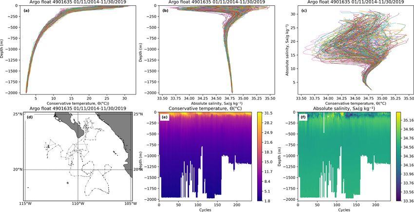
1278                                                                 E. Romero et al.: Filtering method to avoid salinity drifts

Figure 3. Monthly comparison of T –S diagrams of data from RTQC and DMQC. The black boxes delimit the limits of the water masses in
the region and the gray isolines the density (kg m−3 ).

Table 1. Percentages of DMQC and RQTC data admitted and discarded normally and by the two proposed filters.

                                              Without filter           First filter          Second filter
                       Data                 Meas.              %    Meas.             %     Meas.            %
                       DMQC                594 385     69.96 %     594 385     69.96 %    594 385     69.96 %
                       Admitted RTQC             0      0.00 %     209 392     24.64 %     82 196      9.67 %
                       Discarded RTQC      255 184     30.03 %      45 792      5.39 %    172 988     20.36 %
                       Total               849 569   100.00 %      849 569    100.00 %    849 569    100.00 %

   In the results of the Alboran Sea, the westernmost part of        salinity drifts, so in this case it is recommended to use this
the Mediterranean Sea, there are no data deeper than 1500 m          filter and eliminate outliers. In the fourth study area, which
or salinity drifts, so the algorithm directly returns the data       surrounds a central Pacific archipelago, there are many out-
set without modification. The algorithm receives the depth of        liers in all the months; however, the first filter managed to
1500 m by default, and sending a lower depth could eliminate         rule out the salinity drifts present in the months of Septem-
salinity variations if there were any. In the case of Antarc-        ber to December. In this case it is recommended to reduce the
tica, we found that the months of February and April con-            study area into smaller areas to apply the filters and treat the
tain salinity drifts, which could not be completely eliminated       outliers separately. Finally, the large study area located next
with the first filter. For this case, it is recommended to use       to Indonesia shows salinity drifts in the months of March and
the RTQC data supported by the second filter. On the other           July to December. The first filter was able to filter the salinity
hand, in the Bermuda Triangle, salinity drifts are shown in          drifts except for the month of December, because the devia-
the months of June to October, in addition to atypical values        tions are above 1500 m. In this case it is recommended to
in the rest of the months. The first filter already eliminates

Ocean Sci., 17, 1273–1284, 2021                                                           https://doi.org/10.5194/os-17-1273-2021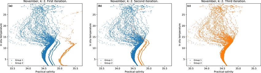
E. Romero et al.: Filtering method to avoid salinity drifts                                                                          1279

Figure 4. Cluster analysis results. Panels (a) and (b) show the groups formed with the RTQC data measured at depths greater than 1500 m.
Panels (c) and (d) show these same grouped data but matched data with the rest of their profile data.

Figure 5. First three iterations of the proposed algorithm using the data for the month of November. Panels (a), (b) and (c) are the first,
second and third interactions.

use the data from the first filter for the months of January to         line represents the given polygon, and the locations of the fil-
November, or use only the months with no outliers.                      tered profiles inside and outside the polygon are represented
                                                                        by dots in red and black respectively.
3.1   Web application                                                      Once the data have been downloaded and transformed, sta-
                                                                        tistical data specific to the EEZ of Mexico can be obtained,
The web application got interesting results and can be ac-              such as the number of profilers within the polygon, the num-
cessed through the cluster_qc library repository. In Fig. 7,            ber of profiles or profilers per year, or the DACs to which
it is observed that the PIP algorithm filters the profiles that         these profilers belong, among others. Table 3 shows the pro-
were made within the EEZ of Mexico correctly. The blue                  filers that have carried out measurements within the poly-

https://doi.org/10.5194/os-17-1273-2021                                                              Ocean Sci., 17, 1273–1284, 2021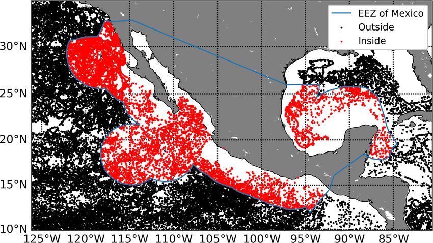
1280                                                                    E. Romero et al.: Filtering method to avoid salinity drifts

Figure 6. Monthly comparison of the T –S diagrams of RTQC and DMQC. (a) First filtering of RTQC. (b) Second filtering of RTQC.

Table 2. Results of Algorithm 1 in five study areas.

                                        DMQC                RTQC – original          RTQC – first filter       RTQC – second filter
                                     Meas.             %      Meas.           %        Meas.             %          Meas.               %
           Alboran Sea              49 401    54.96 %         40 481   45.04 %         40 481      45.04 %        40 481     45.04 %
           Antarctica            1 117 571    92.14 %         95 346    7.86 %         93 647       7.72 %        92 204      7.60 %
           Bermuda Triangle      2 060 348    70.49 %        862 455   29.51 %        468 483      16.03 %       243 752      8.34 %
           Hawaii                3 252 097    70.81 %      1 340 462   29.19 %      1 308 773      28.50 %     1 259 247     27.42 %
           Indonesia             5 260 566    86.86 %        795 900   13.14 %        780 727      12.89 %       771 874     12.74 %

                                                                        Table 3. Profilers and profiles present in the Mexican EEZ.

                                                                                                     Core           Biogeochemical
                                                                            DAC                 Active   Inactive   Active   Inactive       Profiles
                                                                            AO: AOML               51        114        0          3         32 998
                                                                            IF: CORIOLIS            6          3        0          1          1098
                                                                            ME: MEDS                1          1        0          0            201
                                                                            Total                  58        118        0          4         34 297

                                                                        gon given in the month of November 2019. We can see from
                                                                        the table that there is a shortage of biogeochemical profil-
                                                                        ers within the polygon. These four biogeochemical HAPs are
Figure 7. Filtered geographic locations within the EEZ of Mexico.
                                                                        capable of measuring oxygen in addition to temperature and
The irregular polygon that delimits the EEZ of Mexico and the pro-      salinity, but none of their oxygen data satisfactorily finish the
files measured inside and outside of it are shown.                      quality control process, so they are not available. So we can
                                                                        conclude that within the Mexican EEZ there are no good-
                                                                        quality biogeochemical data from Argo HAPs.

Ocean Sci., 17, 1273–1284, 2021                                                                 https://doi.org/10.5194/os-17-1273-2021
E. Romero et al.: Filtering method to avoid salinity drifts 1281
Figure 8. Diagrams produced by the web application. (a) Profile of conservative temperature. (b) Profile of absolute salinity. (c) T –S
diagram. (d) HAP trajectory. (e) Profile of conservative temperature with respect to time. (f) Profile of absolute salinity with respect to time.
For each of these profilers their profiles of temperature salinities outside the global and regional ranges. Therefore,
(Fig. 8a) and salinity (Fig. 8b), the temperature–salinity (T – the quality established by the flags does not take these drifts
S) diagram (Fig. 8c), the estimation of the profiler trajectory into account. A possible solution is for the interested user to
(Fig. 8d), and the profiles of temperature (Fig. 8e) and salin- apply the DMQC on their own (Wong et al., 2021). This pro-
ity (Fig. 8f) with respect to time were generated. These dia- cess can be long and tedious, and for this reason and under
grams are basic for analysis in scientific ocean research. The Argo’s recommendation to use only DMQC for scientific re-
profiler 4901635 is shown as an illustrative example in Fig. 8. search, a large number of users who use the data from Argo
The satellite map of the web application is interactive. It HAPs prefer to directly discard the RTQC data and only use
shows the active and inactive HAPs; filters the data; shows the DMQC data.
statistics, trajectories and diagrams (Fig. 9a); and has other The data in DMQC are consistent with other international
tools to facilitate the visualization and management of the databases such as WOA18 within the study area delimited by
data, such as displaying statistics of a given study area within the irregular polygon, which validates this process. However,
the main polygon (Fig. 9b and c). too much data have to be discarded due to the drifts present
Finally, the filtering of RTQC data that have patterns sim- in RTQC. The filtering proposed in this work is based on
ilar to DMQC data is offered in the web application, which using the patterns followed by the DMQC data to filter the
allows the data to be filtered in a study area within the EEZ RTQC data, especially useful for areas where there are few
of Mexico. It is not necessary to have programming knowl- profiles. This process is carried out by zone and by month,
edge. Access to the web application is through the cluster_qc and in this way it does not matter if the study area is close to
library repository. the arctic or the tropics. The filtering of the RTQC data are
carried out based on the characteristics of the area reflected
in the DMQC data. In addition, when separating the data by
4 Discussion month, their seasonal changes are taken into account. This
means that the resulting RTQC data will have a high proba-
Despite the existence of reports on salinity drifts such as bility of being accepted when the DMQC is applied to them.
the one announced by Argo Data Management (2020) on The time it takes for a modern computer to do cluster anal-
25 September 2018, the quality control processes in real time ysis is relatively short compared to the 12 months it can take
are not yet robust enough to identify them, since these pro- to perform the DMQC, and this will help users interested in
cesses are automatic and mainly look for impossible data, recent data from HAPs to have greater reliability when using
for example, latitudes greater than 90◦ or temperatures and RTQC data. Two filters are proposed: the first is the result
https://doi.org/10.5194/os-17-1273-2021 Ocean Sci., 17, 1273–1284, 20211282 E. Romero et al.: Filtering method to avoid salinity drifts Figure 9. Web application. (a) Data, charts and trajectory of a HAP. (b) HAP trajectories filtered by a drawn polygon. (c) Profiler data within the polygon. of using cluster analysis on the data and the second discards filter by polygons in rectangle or square shape without rota- the HAPs that have presented salinity drifts in the result of tion. the first filter. Therefore the second filter is more reliable but Another platform called OceanOPS (2021) (Joint Centre contains a smaller amount of data. As seen in the TPCM ex- for Oceanography and Marine Meteorology in situ Observa- ample, the user is free to use either one or a combination of tions Programmes Support) does perform statistical analyses both. For example, as seen in Fig. 6a and b, where around on the data; nevertheless this one performs them globally, and 80 % and 30 % of the total discarded data are admitted, the it is not possible to choose a smaller area, for example, only months of July to September continued with salinity drifts af- the EEZ of Mexico or the tropical Pacific off central Mexico ter applying the first filter, to take advantage of more data the and surrounding areas, to obtain statistical information on it. user can use the data from the months of July to September of It is worth mentioning that said platform has a large num- the second filter and the rest of the months use the data from ber of statistics for each variable registered within the source the first. However, as shown by the five study areas used as files; however, being able to generate graphs and tables in an extra example, the percentage of data admitted by the fil- real time using an irregular polygon defined by the user (as ters depends on the study area and its characteristics. It is the shown in this work with the PIP algorithm) would be a great responsibility of the users to make the decision based on their tool for studying these data. knowledge of the study area, which filter to use, if the study The web application described in this document tries to area should be resized or if the default depth value should be cover some of the aforementioned problems and include changed. some of their characteristics, in addition to proposing unpub- There are platforms to access data from Argo HAPs, such lished options such as filtering by irregular polygons, statis- as Argo Data Management (2020), Coriolis (2020) and Euro- tics adaptable to filters, generation of graphs according to Argo (2020) in addition to other options such as FTP or snap- user needs and RTQC data filtering. However, the web ap- shots. The current platforms already provide graphics and plication is in its initial phase, and there are still many tools data from the profilers, as well as filters to display or down- and databases that can be integrated to offer an even more load the data. However, the geographical filter they use is by complete experience. maximum and minimum coordinates, so it is only possible to Ocean Sci., 17, 1273–1284, 2021 https://doi.org/10.5194/os-17-1273-2021
E. Romero et al.: Filtering method to avoid salinity drifts                                                                             1283

5   Conclusions                                                         supervised this work. LTF, IC and MC contributed to the conceptu-
                                                                        alization and design of the study, the interpretation of the data, and
                                                                        the preparation of the article.
This work gives two filtering methods to discard only the
RTQC data that present salinity drifts and with it to take ad-
vantage of the largest amount of data within a given polygon.
                                                                        Competing interests. The authors declare that they have no conflict
In the TPCM, from the total RTQC data it was possible to re-
                                                                        of interest.
cover around 80 % in the case of the first filter and 30 % in the
case of the second, which are usually discarded due to prob-
lems such as salinity drifts. This allows users to use any of           Disclaimer. Publisher’s note: Copernicus Publications remains
the filters or a combination of both to have a greater amount           neutral with regard to jurisdictional claims in published maps and
of data within the study area of their interest in a matter of          institutional affiliations.
minutes, rather than waiting for the DMQC that takes up to
12 months to be completed.
   This work provides useful tools to increase productivity in          Acknowledgements. We are grateful to CONACYT for granting
scientific investigations that use data from the water column.          scholarship no. 731303 to Emmanuel Romero. We appreciate that
The PIP algorithm turns out to be an efficient method to di-            these data were collected and made freely available by the Inter-
rectly filter the data from any georeferenced database using            national Argo Program and the national programs that contribute
geographic locations, while the algorithms proposed for fil-            to it (https://argo.ucsd.edu (last access: January 2020) https://www.
tering RTQC data allow the separation of the data not yet               ocean-ops.org, last access: April 2021). The Argo Program is part
                                                                        of the Global Ocean Observing System. We also thank the Insti-
adjusted by the DMQC into data with salinity drifts and data
                                                                        tuto Tecnológico de La Paz (ITLP) and the Centro Interdiciplinario
that show patterns similar to those of the DMQC data, in or-            de Ciencias Marinas (CICIMAR) for their institutional support. We
der to increase the amount of data in study areas with scarce           also acknowledge the critical comments from the reviewers.
data from HAPs. Finally, the web app demonstrates one of
the applications in which these proposals can be used.
                                                                        Financial support. This research has been supported by CONA-
                                                                        CYT (scholarship no. 731303).
Code availability. cluster_qc was developed in Python 3.7 and is
licensed under a Creative Commons Attribution 4.0 International
License. The source code is available at https://doi.org/10.5281/       Review statement. This paper was edited by Oliver Zielinski and
zenodo.4595802 (Romero et al., 2021a). The latest package version       reviewed by two anonymous referees.
is v1.0.2.

Data availability. These data were collected and made freely avail-
able by the International Argo Program and the national pro-            References
grams that contribute to it: https://argo.ucsd.edu (last access: Jan-
uary 2020, Argo, 2020a) and https://www.ocean-ops.org (last ac-         Argo: Argo [data set], available at: https://argo.ufcsd.edu/, last ac-
cess: April 2021, OceanOPS, 2021). The Argo Program is part                cess: January 2020a.
of the Global Ocean Observing System. The data were down-               Argo: Argo float data and metadata from Global Data Assembly
loaded from the Coriolis GDAC FTP server in 2019, and the                  Centre (Argo GDAC) – Snapshot of Argo GDAC of Decem-
snapshot from December 2020 (Argo, 2020b) was also used. The               ber 10st 2020, [data set], https://doi.org/10.17882/42182#79118,
data used from the NCEI World Ocean Database 2018 are the                  2020b.
monthly data of temperature (https://www.ncei.noaa.gov/products/        Argo Data Management Team: Argo user’s manual V3.3, Report,
world-ocean-database, last access: November 2019, Locarnini                https://doi.org/10.13155/29825, 2019.
et al., 2018) and salinity (https://www.ncei.noaa.gov/products/         Argo Data Management: Argo Data Management, available at: http:
world-ocean-database, last access: November 2019, Zweng et al.,            //www.argodatamgt.org/, last access: 2020.
2018) of the statistical mean of each quarter of a degree (1/4◦ )       Coriolis: Coriolis: In situ data for operational oceanography, avail-
from 2005 to 2017. Maps throughout this work were created us-              able at: http://www.coriolis.eu.org/, last access: 2020.
ing ArcGIS® software by Esri. ArcGIS® and ArcMap™ are the               Euro-Argo: Argo Fleet Monitoring – Euro-Argo, available at: https:
intellectual property of Esri and are used herein under license.           //fleetmonitoring.euro-argo.eu/, last access: 2020.
Copyright © Esri. All rights reserved. For more information about       Everitt, B., Landau, S., Leese, M., and Stahl, D.: Cluster Analysis,
Esri® software, please visit https://www.esri.com/en-us/home (last         Wiley Series in Probability and Statistics, Wiley, 346 pp., 2011.
access: November 2019).                                                 Fiedler, P. and Talley, L.: Hydrography of the Eastern
                                                                           Tropical Pacific: a review, Prog. Ocean., 69, 143–180,
                                                                           https://doi.org/10.1016/j.pocean.2006.03.008, 2006.
Author contributions. ER developed the methodology and software         Godínez, V. M., Beier, E., Lavín, M. F., and Kurczyn, J. A.: Circu-
described in this work and also performed the data analysis. LTF           lation at the entrance of the Gulf of California from satellite al-

https://doi.org/10.5194/os-17-1273-2021                                                               Ocean Sci., 17, 1273–1284, 2021
1284 E. Romero et al.: Filtering method to avoid salinity drifts timeter and hydrographic observations, J. Geophys. Res.-Oceans, Portela, E., Beier, E., Barton, E., Castro Valdez, R., Godínez, 115, C04007, https://doi.org/10.1029/2009JC005705, 2010. V., Palacios-Hernández, E., Fiedler, P., Sánchez-Velasco, L., Hartigan, J. A. and Wong, M. A.: Algorithm AS 136: A K- and Trasviña-Castro, A.: Water Masses and Circulation in the Means Clustering Algorithm, J. R. Stat. Soc., 28, 100–108, Tropical Pacific off Central Mexico and Surrounding Areas, https://doi.org/10.2307/2346830, 1979. J. Phys. Ocean., 46, 3069–3081, https://doi.org/10.1175/JPO-D- Foley, J. D., van Dam, A., Feiner, S. K., and Hughes, J. F.: Com- 16-0068.1, 2016. puter Graphics: Principles and Practice, The Systems Program- Romero, E., Tenorio-Fernandez, L., Castro, I., and Cas- ming Series, Addison-Wesley, 2 Edn., 1175 pp., 1990. tro, M.: romeroqe/cluster_qc: Filtering Methods based Kessler, W. S.: The circulation of the eastern tropi- on cluster analysis for Argo Data, Zenodo [code], cal Pacific: A review, Prog. Ocean., 69, 181–217, https://doi.org/10.5281/zenodo.4595802, 2021a. https://doi.org/10.1016/j.pocean.2006.03.009, 2006. Romero, E., Tenorio-Fernandez, L., Castro, I., and Castro, Lavín, M., Beier, E., Gomez-Valdes, J., Godínez, V., M.: Argo data filtering results to avoid salinity drifts, and García, J.: On the summer poleward coastal cur- https://doi.org/10.6084/m9.figshare.14999613.v1, 2021b. rent off SW México, Geophys. Res. Lett, 33, L02601, Stramma, L., Johnson, G. C., Sprintall, J., and Mohrholz, V.: Ex- https://doi.org/10.1029/2005GL024686, 2006. panding Oxygen-Minimum Zones in the Tropical Oceans, Sci- Lavín, M. F. and Marinone, S. G.: An Overview of the Physical ence, 320, 655–658, https://doi.org/10.1126/science.1153847, Oceanography of the Gulf of California, Springer Netherlands, 2008. 173–204, https://doi.org/10.1007/978-94-010-0074-1_11, 2003. Wong, A., Keeley, R., and Carval, T.: Argo Quality Control Lavín, M. F., Castro, R., Beier, E., Godínez, V. M., Amador, A., Manual for CTD and Trajectory Data, Report, USA, France, and Guest, P.: SST, thermohaline structure, and circulation in https://doi.org/10.13155/33951, 2021. the southern Gulf of California in June 2004 during the North Zamudio, L., Leonardi, A., Meyers, S., and O’Brien, J.: ENSO and American Monsoon Experiment, J. Geophys. Res.-Oceans, 114, Eddies on the Southwest cost of Mexico, Geophys. Res. Lett., 28, C02025, https://doi.org/10.1029/2008JC004896, 2009. 2000GL011814, https://doi.org/10.1029/2000GL011814, 2001. Locarnini, R., Mishonov, A., Baranova, O., Boyer, T., Zweng, M., Zamudio, L., Hurlburt, H., Metzger, E., and Tilburg, C.: Trop- Garcia, H., Reagan, J., Seidov, D., Weathers, K., Paver, C., Smol- ical Wave-Induced Oceanic Eddies at Cabo Corrientes and yar, I., and Locarnini, R.: World Ocean Atlas 2018, Volume the Maria Islands, Mexico, J. Geophys. Res., 112, 18, 1: Temperature, edited by: Mishonov, A., NOAA Atlas NES- https://doi.org/10.1029/2006JC004018, 2007. DIS [data set], available at: https://www.ncei.noaa.gov/products/ Zweng, M., Reagan, J., Seidov, D., Boyer, T., Locarnini, R., world-ocean-database (last access: November 2019), 1, 52 pp., Garcia, H., Mishonov, A., Baranova, O., Paver, C., and 2018. Smolyar, I.: World Ocean Atlas 2018 [data set], Volume OceanOPS: OceanOPS [data set], available at: https://www. 2: Salinity, available at: https://www.ncei.noaa.gov/products/ ocean-ops.org, last access: April 2021. world-ocean-database (last access: November, 2019), edited by: Pantoja, D., Marinone, S., Pares-Sierra, A., and Gomez-Valdivia, Mishonov, A., NOAA Atlas NESDIS, 50 pp., 2018. F.: Numerical modeling of seasonal and mesoscale hydrography and circulation in the Mexican Central Pacific, Cienc. Mar., 38, 363–379, https://doi.org/10.7773/cm.v38i2.2007, 2012. Ocean Sci., 17, 1273–1284, 2021 https://doi.org/10.5194/os-17-1273-2021
You can also read