The Resistance to Label Noise in K-NN and DNN Depends on its Concentration - BMVC 2020
←
→
Page content transcription
If your browser does not render page correctly, please read the page content below
DRORY, RATZON, AVIDAN, GIRYES: LABEL NOISE IN K-NN AND DNN                                           1

The Resistance to Label Noise in K-NN and
DNN Depends on its Concentration
Amnon Drory                                                 Tel-Aviv University
amnondrory@mail.tau.ac.il                                   Israel
Oria Ratzon
oriaratzon1@gmail.com
Shai Avidan
avidan@eng.tau.ac.il
Raja Giryes
raja@tauex.tau.ac.il

                                                     Abstract
           We investigate the classification performance of K-nearest neighbors (K-NN) and deep
       neural networks (DNNs) in the presence of label noise. We first show empirically that a
       DNN’s prediction for a given test example depends on the labels of the training examples
       in its local neighborhood. This motivates us to derive a realizable analytic expression
       that approximates the multi-class K-NN classification error in the presence of label noise,
       which is of independent importance. We then suggest that the expression for K-NN may
       serve as a first-order approximation for the DNN error. Finally, we demonstrate empirically
       the proximity of the developed expression to the observed performance of K-NN and
       DNN classifiers. Our result may explain the already observed surprising resistance of
       DNN to some types of label noise. It also characterizes an important factor of it showing
       that the more concentrated the noise the greater is the degradation in performance.

1     Introduction
Deep neural networks (DNN) provide state-of-the-art results in many computer vision chal-
lenges, such as image classification [25], detection [40] and segmentation [5]. Yet, to train
these models, large datasets of labeled examples are required. Time and cost limitations come
into play in their creation, which often result in imperfect labeling, or label noise, due to
human error [18]. An alternative to manual annotation are images taken from the Internet that
use the surrounding text to produce labels [55]. This approach results in noisy labels too.
    Perhaps surprisingly, it has been shown [24] that DNNs trained on datasets with high
levels of label-noise may still attain accurate predictions. This phenomenon is not unique
only to DNNs but also to classic classifiers such as K-Nearest Neighbours (K-NN) [1, 8, 34].
    Fig. 1 demonstrates this behavior. It shows the 10 MNIST classes, using deep features
embedded in 2-dimensional space with t-SNE [54]. We change the labels of a randomly
selected 20% of the training data. A network trained with this noisy data is capable of reaching
100% prediction accuracy. On the other hand, it also shows the case where concentrated
 c 2020. The copyright of this document resides with its authors.
It may be distributed unchanged freely in print or electronic forms.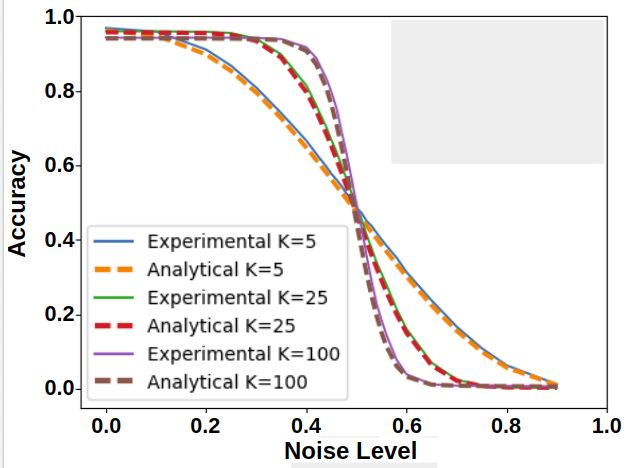
2                     DRORY, RATZON, AVIDAN, GIRYES: LABEL NOISE IN K-NN AND DNN

Figure 1: Effect of label noise type: Each cluster represents a class and the color represents the label
provided for each data point. (left) 20% uniformly spread random noise. The network achieves ∼ 100%
prediction accuracy. (right) 20% locally concentrated noise. The network achieves ∼ 80% accuracy.

groups of examples have all their labels flipped to the same label. Here too, 20% are changed,
but the noise is no longer distributed uniformly in the example set space but is instead is
locally concentrated. In this case, the DNN does not overcome the noise and accuracy drops
to 80%. Clearly, the type of label noise is as important as its amount.
    The starting point of this work is the observation that a DNN’s prediction for any given
test example depends on a local neighborhood of training examples, where local is in some
implicit space. We indirectly demonstrate this by injecting varying levels of a known noise
into the training set, and measuring the effect - first on the softmax output of the network, and
secondly on accuracy-vs-noise-level curves.
    The output of a classification DNN’s last-layer, the softmax layer, is a probability distribu-
tion over the possible labels. We show that when noise is added, these distributions tend to
encode the distribution of labels of training examples in a local neighborhood around a test
example. This means that the output of a DNN is similar to the output of a K-NN algorithm
performed in some implicit space. Motivated by this, we are able to develop an analytical
expression for the expected accuracy of a K-NN algorithm given a noisy training set, when
the parameters of the noise producing process are known. This allows us to produce analytical
accuracy-per-noise-level curves. Next, we actually produce noisy training sets with varying
levels of noise, train a DNN on each, and measure its accuracy. This results in experimental
accuracy-per-noise-level curves for DNNs. By comparing the analytical and experimental
curves, we demonstrate that the K-NN model is a good first order prediction for the behaviour
of DNNs in the presence of noise. This is an important step forward in understanding DNN’s
resistance to label noise. It also allows us to recognize a very important factor governing
the extent to which DNNs can resist label noise: whether the noise is randomly spread or
locally concentrated in the training set. When label noise is randomly spread, the resistance
to noise is high, since the probability of noisy examples overcoming the correct ones in any
local neighborhood is small. However, when the noisy examples are locally concentrated,
DNNs are unable to overcome the noise.
    Our findings are also motivated by recent works that show that networks perform a smooth
interpolation between the labels of training examples [11, 36, 45, 57]. We suggest using
K-NN as a first order approximation of such an interpolation.
   We validate our analytical expression both for K-NN and DNN using extensive exper-
iments on several datasets: MNIST, CIFAR-10, and ImageNet ILSVRC. We show that
empirical curves of accuracy-per-noise-level fit well with our mathematical expression.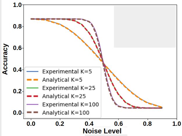
DRORY, RATZON, AVIDAN, GIRYES: LABEL NOISE IN K-NN AND DNN                                      3

2    Related Work
Classification in the presence of label noise has long been explored in the context of classical
machine learning [1, 8, 34]. We focus on K-NN robustness and its implication on DNN.
     K-NN label-noise robustness. K-NN sensitivity to label noise has been discussed in
multiple works [44, 58]. Prasath et al. [39] show an impressive resistance of K-NN to uniform
label noise: drop of only 20% for 90% noise level. Tomašev and Buza [52] observe that
resistance to noise depends on its type. They present the hubness-proportional noise model,
where the probability of an example being corrupted depends not only on its label, but also
on its nearness to other examples, and show that this noise is harder for K-NN than uniform
noise.
     The closest K-NN theory to ours is [35], which provides an expression for the K-NN
accuracy as a function of noise level. Their derivation relies on the particulars of a specific
setting, namely a binary classification task where the inputs are binary strings and the output is
1 if a majority of relevant places in the string are set to 1. Our work can be seen as expanding
and generalizing their derivation, as it handles: (i) general input domains; (ii) multi-class
classification (not just 2 classes); and (iii) a much more complex family of noise models.
     DNN label-noise robustness. The effect of label noise on neural networks has been
studied as well. Several works, e.g. [7, 24, 43, 49] have shown that neural networks trained
on large and noisy datasets can still produce highly accurate results. For example, Krause
et al. [24] report classification results on up to 10, 000 categories. Their key observation is
that working with large scale datasets that are collected by image search on the web leads to
excellent results even though such data is known to contain noisy labels.
     Sun et al. [49] report logarithmic growth in performance as a function of training set size.
They perform their experiments on the JFT-300M dataset, which has more than 375M noisy
labels for 300M images. The annotations have been cleaned using complex algorithms. Still,
they estimate that as much as 20% of the labels are noisy and they have no way of detecting
them. Wang et al. [56] investigate label-noise in face recognition and its impact on accuracy.
     In [3, 12], an extra noise layer is introduced to the network to address label noise. It is
assumed that the observed labels were created from the true labels by passing through a noisy
channel whose parameters are unknown. They simultaneously learn the network parameters
and the noise distribution. Another approach [22, 28, 53, 59] models the relationships between
images, class labels and label noise using a probabilistic graphical model and further integrate
it into an end-to-end deep learning system. Other methods that show that training on additional
noisy data may improve the results appear in [6, 13, 26, 27, 29].
     Several methods “clean-up” the labels by analyzing given noisy labeled data [14, 15,
19, 23, 42, 46, 50, 51]. For example, Reed et al. [41] combat noisy labels by means of
consistency. They consider a prediction to be consistent if the same prediction is made
given similar percepts, where the notion of similarity is between deep network features
computed from the input data. Malach and Shalev-Schwartz [32] suggest a different method
for overcoming label noise. They train two networks, and only allow a training example to
participate in the stochastic gradient descent stage of training if these networks disagree on
the prediction for this example. This allows the training process to ignore incorrectly labeled
training examples, as long as both networks agree about what the correct label should be.
     Liu et al. [30] propose to use importance reweighting to deal with label noise in DNN.
They extend the idea of using an unbiased loss function for reweighting to improve resistance
to label noise in the classical machine learning setting [1, 8, 34]. Another strategy suggests to
employ robust loss functions to improve the resistance to label noise [9, 10, 20, 21, 37, 61].
4                       DRORY, RATZON, AVIDAN, GIRYES: LABEL NOISE IN K-NN AND DNN

In [60] an extra variable is added to the network to represent the trustworthiness of the labels,
which helps improving the training with noisy labels. Ma et al. [31] study the dimensionality
of the learned representations of examples with clean and noisy labels. They show that there
is a difference in the dimensionality between the two cases and use it to improve the training.
This work studies the embedding space of trained networks and show a relationship to K-NN.
We use this relationship to provide a first-order estimate for DNN resistance to label noise.

3     Analysis of Robustness to Label Noise
We take the following strategy to analyze label noise: First, we establish the different label
noise models to consider. Then we show empirically that the output of the DNN’s softmax
resembles the label distribution of the K nearest neighbors, linking DNNs to the K-NN
algorithm. With this observation in hand, we derive a formula for K-NN, which is of interest
by itself, with the hypothesis that it applies also to DNN.
Setting. In the “ideal” classification setting, we have a training set T = {xi , yi }Ni=1 and a
test set S = {x̂i , ŷi }M  i=1 , where x is typically an image, and y is a label from the label set
L = {`1 , `2 , . . . , `L }. A classification algorithm (DNN or K-NN) learns from T and is tested
on S. The setting with label noise is similar, except that the classifier learns from a noisy
training set {xi , ỹi }Ni=1 , which is derived from the clean data T by changing some of the labels.
We designate by γ the fraction of training examples that are corrupted (with changed labels).1
    An often studied noise setting is that of randomly-spread noise. In this setting the process
of selecting the noisy label ỹ is agnostic to the content of the image x, and instead only
depends (stochastically) on the clean label y. The examples that get corrupted (i.e. their labels
are changed) are selected uniformly at random from the training set T . For each such example,
the noisy label is stochastically selected according to a conditional probability P(ỹ|y) (we
refer to this as the corruption matrix).2 This setting can capture the overall similarity in
appearance between categories of images, which leads to error in labeling.
    Two simple variants of randomly spread noise are often used: Uniform Noise, and Flip-
Noise. Uniform Noise is the case where the noisy label is selected uniformly at random from
L. This corresponds to a corruption matrix where P(ỹ|y) = L1 for all ỹ, y. In the flip label-noise
setting, each label `i has one counterpart ` j with which it may be replaced. In this case each
row in the corruption matrix has exactly one entry that is 1, and the rest are 0.
    In contrast with the randomly spread setting, we also consider the locally concentrated
noise setting, where the noisy labels are locally concentrated in the training set [17]. As
an example, consider a task of labeling images as either cat or dog, and a human annotator
that consistently marks all poodles as cat. We show that K-NN and, by extension DNN, are
resilient to randomly spread label noise but not to locally concentrated one.

3.1     The Connection Between DNN and K-NN.
We observe that DNN’s prediction, similar to K-NN, tends to be the plurality label (the most
common label) in a local neighborhood of train examples that surround the test example. The
connection between K-NN and DNN is observed indirectly, by adding different types of noise
   1 Note that the subset of "corrupted" examples may actually contain examples whose label has not changed. This

happens when the randomly selected noisy label happens to be the same as the original label.
   2 A confusion matrix C can be derived from the corruption matrix by C = (1−γ)I + γP, where I is the identity

matrix.
DRORY, RATZON, AVIDAN, GIRYES: LABEL NOISE IN K-NN AND DNN                                      5

to the training set, and analyzing its effect on the network’s softmax-layer output. We find
that this output tends to be the local probability distribution of the training examples in the
vicinity of x. Therefore, its argmax ` pred = arg max{so f tmaxx (`)} tends to be the plurality
                                                   `∈L
label.
     Fig. 2 presents the average softmax output of DNNs for various noise types and datasets.
It demonstrates how the softmax layer output tends to be the distribution of the labels in the
neighborhood of training examples. For example, when there is a uniform noise with noise
level γ, we see that the value of the softmax is approximately Lγ everywhere except at the peak
location. This is indeed the expected fraction of noisy examples from each class in any given
local neighborhood. In the case of flip noise, it can be seen that the softmax probabilities are
mostly concentrated at the correct class and the alternative class, and that the alternative class
probability is approximately at the noise level. Additional softmax diagrams for MNIST and
CIFAR-10 can be found in the supplementary material.
     It follows that the network makes a wrong prediction only when the “wrong” class achieves
plurality in a local neighborhood. This, for example, is the case when locally concentrated
noise is added and the test example is taken from the noisy region.
     These findings provide us with an intuition into how DNNs are able to overcome label
noise: Only the plurality label in a neighborhood determines the output of the network.
Therefore, adding label noise in a way that does not change the plurality label should not
affect the network’s prediction. As long as the noise is randomly spread in the training set,
the plurality label is likely to remain unchanged. The higher the noise level, the more likely
it is that a plurality label switch will occur in some neighborhoods. When the noise type
and noise level are known, we are able to produce a mathematical expression for the K-NN
model, that approximately predicts the probability of a switch. We suggest that this can
serve as a first-order approximation to the behaviour of DNNs in the presence of noise. We
show empirically that indeed it does match the observed behaviour of DNNs quite well in
some settings. We also believe that this expression for K-NN is of independent interest, as it
improves and extends previously known mathematical models for the resistance of K-NNs to
noise [35].
     For the most part, our analysis does not require us to explicitly specify the space in which
distance between examples is defined. Our mathematical derivation of expected accuracy-per-
label-noise curves does not rely on any of these specifics, but instead only on the parameter
K, and knowledge of the noise producing process. The fact that the analytical curves match
quite well with the experimental curves for DNN, demonstrates the relation between K-NN
and DNN. Similarly, no explicit specification of the space is needed to demonstrate the effect
of the noise on the DNN’s softmax layer output.
     A specific embedding space of interest is the output of the penultimate layer of a trained
network, since distances between examples in this space are expected to carry some semantic
meaning. In the supplementary material we describe an experiment that demonstrates the
similarity between K-NN in this space, and softmax layer outputs.

3.2 K-NN Accuracy in The Randomly-Spread Noise Setting.
We turn to produce an analytical expression for the probability of a plurality switch, in the
randomly-spread noise setting.
    We model randomly spread noise as follows: each test example (x̂s , ŷs ) has a local
neighborhood N (x̂s ) of K training examples. qi is the probability for any example in N (x̂s ) to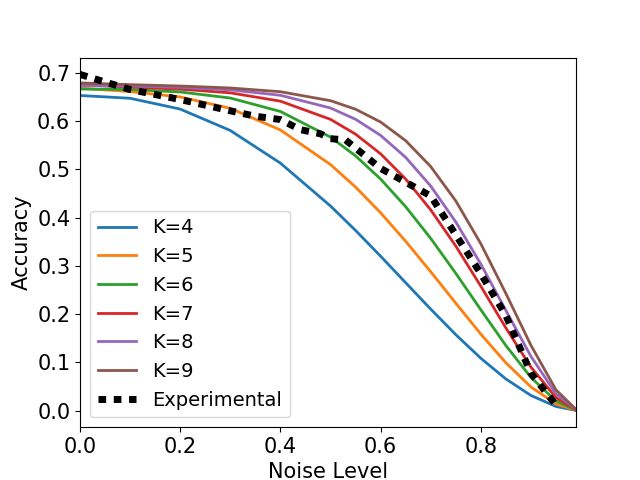
6                    DRORY, RATZON, AVIDAN, GIRYES: LABEL NOISE IN K-NN AND DNN

(a) CIFAR-10, 30% uni-     (b) CIFAR-10, 40% flip        (c) MNIST, Locally con-              (d) MNIST, Locally
form noise                 noise                         centrated noise, example             concentrated noise,
                                                         in a clean region                    example in a noisy
                                                                                              region
Figure 2: Softmax analysis: Each diagram is aggregated from many test examples. The height of the
bars shows the median, and the confidence interval shows the central 50% of examples. The ground
truth label is marked by a black margin. Additional softmax diagrams are found in the supplemental
material.

have the observed label `i . The distribution q encodes the results of the noise-creation process,
and it depends on the parameters of this process, and on the clean labels of the examples
in N (x̂s ). Following [35] we considerably simplify our derivation by introducing a small
approximation: instead of treating the clean training examples as constant, we consider them
to be sampled i.i.d from a clean distribution Cs (`). The K-NN algorithm’s prediction, which
we denote by Y (x̂s ), is the plurality label. Its expected accuracy is defined as follows.
Definition 1 (K-NN Prediction Accuracy). K-NN prediction accuracy is defined as

                                                 1 M
                                 AK−NN ,           ∑   Pr Y (x̂s ) = ŷs ,                                       (1)
                                                 M s=1

where Pr Y (x̂s ) = ŷs is the probability that the plurality label of test example x̂ in N (x̂) is
the same as the ground truth label for x̂.
    By expanding the expression in Eq. (1), we obtain an analytical formula for the accuracy
of a K-NN classifier, which is given in the following theorem (proof in the sup. material):
Theorem 1 (Plurality Accuracy). The probability of the plurality label being correct is

                                                                           K
                                                                                           · qn11 · · · qnLL ,

           Q , Pr Y (x̂) = ŷ = ∑ ∑ · · · ∑ Jni >n j , ∀ j6=iK ·                                                 (2)
                                  n1 n2     nL                      n1 , n2 , . . . , nL

where J·K is the indicator function, ŷ = `i is the correct label, n j is the number of appearances
of the label ` j in N (x̂) and q j is the probability of any such appearance.
    What is left to show is how to calculate q j . The probability q j is derived from the process
that creates the noisy training set. Let x̂s be a test example, and let x be a training example in
N (x̂s ). Let y be the clean label of x and ỹ be its noisy label. We denote by Cs (`) the clean
label distribution in N (x̂s ). In other words, Cs (`) , Pr(y = `). Thus, the expression for q j is
                                                                L
               q j , Pr(ỹ = ` j ) = (1−γ) ·Cs (` j ) + γ · ∑ P(` j |`k ) ·Cs (`k ),                             (3)
                                                              k=1

where γ is the noise level, and P(ỹ|y) is the corruption matrix that defines the corruption
process. Eq. (3) shows that an example may be labeled with a noisy label ` in two ways: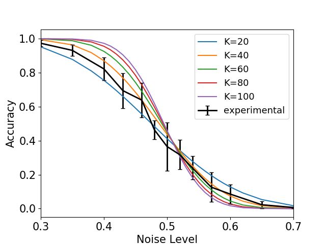
DRORY, RATZON, AVIDAN, GIRYES: LABEL NOISE IN K-NN AND DNN 7
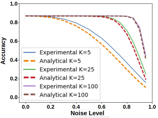
(a) MNIST flip (b) CIFAR-10 flip (c) CIFAR-10 uniform (d) ImageNet uniform
Figure 3: K-Nearest Neighbors Analytical and Experimental curves, showing that the effect of noise
on accuracy is predicted very well by the analytical model. For the MNIST dataset, K-NN is performed
in the space of image pixels (784 dimensions). For the CIFAR-10 dataset, K-NN is performed in a
256-dimensional feature space, derived from a Neural Network that was trained on CIFAR-10. For
ImageNet, K-NN is performed in the 2048 dimensional feature space derived from DenseNet-121.
Either this example is uncorrupted and ` was its original label, or this example was corrupted
and received ` as its noisy label.
We can greatly improve the efficiency of calculating Q by first decomposing the multino-
mial coefficient into a product of binomials, and then decomposing Q into
L−1
M1 ML K − ∑ n j
K n1
Q= ∑ q1 · · · ∑ j=1 qnLL , (4)
n1 =m1 n1 nL =mL nL
where mi is the smallest number of repeats of `i allowed, Mi is the largest, and together
they encode the requirement that ni > n j ∀ j 6= i. See supplementary material for a detailed
derivation. Equation (4) contains many partial sums that are repeated multiple times, which
allows further speedups by dynamic programming.
Estimating the clean distribution: In the K-NN setting, we can find the clean distribution by
simply analyzing the clean data and noting the labels of the examples in the K-neighborhood
of each test example. In the DNN setting, we could do the same by selecting a specific
embedding space in which to measure distances, e.g. the network’s penultimate layer’s output.
However, such an explicit selection is unnecessary: instead, we follow our observations in
Fig. 2 and treat the softmax layer output (of a network trained on clean data) as the clean
distribution. This results in a much more computationally efficient algorithm.
3.3 The Locally-Concentrated Noise Setting.
An approximate analysis of DNN accuracy based on the K-NN algorithm can be done also in
the locally concentrated noise setting. Following our observation that DNN behaves similarly
to K-NN performed in some implicit space, we need to assume that the noisy examples are
concentrated in this space.
If the noise is concentrated, then N (x̂) is almost always contained either in the corrupt
area or clean area. In the first case, the prediction will be based on the corrupt label, therefore
wrong. In the second, it will be correct. Therefore, the expected accuracy can be determined
by the fraction of test examples for which N (x̂) is in the clean area. If we assume that
the test examples are approximately uniformly spread in the example space, we can expect
this fraction to be 1−γ. Figs. 2(c,d) and Fig. 4(h,i) demonstrate that this is indeed the case
empirically.
8                        DRORY, RATZON, AVIDAN, GIRYES: LABEL NOISE IN K-NN AND DNN

             (a) MNIST flip                   (b) CIFAR-10 flip                   (c) ImageNet flip

           (d) MNIST uniform                (e) CIFAR-10 uniform                (f) ImageNet uniform

    (g) MNIST general corruption matrix   (h) MNIST concentrated noise      (i) CIFAR-10 concentrated noise
Figure 4: DNN Analytical and Experimental curves. The experimental curves show the mean accuracy
and standard deviation. In most cases, the experimental curve is quite close to the corresponding
analytical curves, and is clearly different from the analytical curves of the other settings (other subfigures).
In (g) we also show the corruption-matrix P(ỹ|y) (rows are original label, columns are corrupt label, and
brightness denotes probability, where white=high, black=low).

4       Experiments
Our analytical model for K-NN acurracy in the presence of noise provides accuracy-vs-noise
curves. We compare these to experimental curves derived from performing K-NN and DNN
on noisy data. We repeat these experiments with multiple noise types, and several popular
datasets: MNIST, CIFAR-10, and ImageNet (ILSVRC 2012). Notice that we re-train the
network for each dataset, noise type and noise level.
    K-NN experiments: Fig. 3 shows how well Eq. (2) approximates K-NN classification in
practice. We show results for both MNIST and CIFAR-10 for the case of uniform and flip
label noise, and for different k values. As can be seen, our model fits the data well.
For each dataset we use an embedding of the examples in a space that is semantically
meaningful enough to allow successful classification using K-NN. The MNIST dataset is
simple enough that we can simply use the image pixels. For the other datasets, however, we
use the output of the penultimate layer of the DNN trained to classify the dataset (described
hereafter).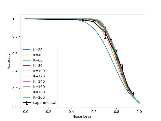
DRORY, RATZON, AVIDAN, GIRYES: LABEL NOISE IN K-NN AND DNN                                      9

     Implementation details: The analytical expressions in Eq. (4) are computationally
intensive. For a feasible run-time, we found it necessary to use a multi-threaded C++ im-
plementation that relies heavily on dynamic programming. On a fast 8-core Intel i7 CPU,
producing the analytical curves for each figure takes up-to 60 minutes.
     To generate the empirical plots, we repeat the following process for different noise levels:
add noise to the training set, train a DNN, and then measure its accuracy on the clean test
set. When it is computationally feasible, we repeat the experiment several times and estimate
the mean accuracy and its standard deviation (10 repeats for MNIST, 7 for CIFAR-10). For
CIFAR-10 and MNIST we use a train/validation split of 90%/10%. The clean validation
set is used for early stopping [38]. We perform this in our experiments to improve the
network performance following the observations in [2, 4]: one effect of overfitting may be
memorization of noisy labels, which could degrade DNN’s resistance to label-noise.
     For all MNIST experiments, we use a DNN, which reaches ∼100% accuracy. Its structure
is described in the sup. material. For the CIFAR-10 experiments, we use the All Convolutional
Network [47]. To produce features for the K-NN experiments, an additional fully connected
layer was added before the softmax, with 256 output channels. For ImageNet experiments,
we use the Densenet-121 [16] architecture, with Adam Optimization and mini-batch of size
256. The feature used in K-NN experiments is 2048-dimensional.
     The results of our experiments are summarized in Fig. 4. They contain four types of noise
(uniform, flipped, general confusion matrix, and locally concentrated), three datasets (MNIST,
CIFAR-10, and ImageNet), and different values of K (i.e., different neighborhood sizes). To
experiment with locally concentrated noise, we need to explicitly select a specific space and
select groups of examples that are concentrated in this space. Specifically, we use the output
of the penultimate layer of a network trained on clean data as a 256-dimensional embedding
space. We use k-means to find clusters of examples that are locally-concentrated in this space.
For each class separately: we divide into k clusters, then we select one cluster and change
all of the labels in it into the same incorrect label. Each class `i has one alternative class ` j
to which the noisy labels are flipped. k-means with different values of k results in different
noise-levels, from roughly 10% when k = 10, to roughly 50% when k = 2.
     Validation of analytical expression: The graphs show that we can calculate analyti-
cally the performance of the network for a given noise level, for some types of label noise.
Specifically, the black line in each graph shows the performance of a network trained with a
growing amount of label noise. The colored line curves show graphs computed analytically
that determine the performance of a network, given different neighborhood sizes. That is, we
show that there is a connection between label noise and neighborhood size. This connection
lets us compute analytically the expected accuracy of a network without having to train it.
In all cases, the experimental curve appears to naturally follow its corresponding family of
analytical curves. We believe this indicates that the analytical curves approximate the general
behavior of the experimental curves. In other words, our mathematical analysis captures a
major factor in explaining the resistance of DNNs to spatially-spread noise. On a smaller
scale, there are some deviations of the experimental curves from the anlytical ones. This
could be caused by secondary factors that are not considered by the model.
     The impact of noise concentration on DNN’s resistance to label noise: The analytical
expression predicts that DNNs may resist high levels of noise, but only if the noise is
randomly spread in the training set (i.e., the uniform and flip settings). In contrast, in the
locally concentrated noise setting DNNs are expected to have no resistance to noise. Note that
indeed, this predicted behavior is demonstrated in the plots. In particular, our experiments
show that the uniform noise setting is easier for the network than the flip setting. In the flip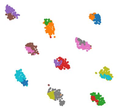
10                   DRORY, RATZON, AVIDAN, GIRYES: LABEL NOISE IN K-NN AND DNN

case, resistance to noise holds only until the noise level approaches 50%. In the uniform noise
setting, noticeable drop in accuracy happens only when approaching 90%. This is due to the
fact that in the flip setting, at 50% there is a reversal of roles between the correct label and
the alternative labels, and the DNN ends up learning the alternative labels while ignoring
the correct ones. In the uniform noise setting, however, the probability of the correct label
being the plurality label is still higher than that of any of the other labels. Note that all these
behaviours are in accordance with our theory.

5    Conclusion
This work studies the robustness of K-NN and neural networks to label noise. We provide
an analytic expression that predicts accurately the resistance of K-NN to label noise and can
be evaluated efficiently. Moreover, we show that the developed formula can also be used to
understand the behavior of neural networks in the presence of different noise types.
    The underlying assumption for using this term also for trained neural networks is that they
behave similarly to K-NN. This assumption is related to recent studies of the function space
of neural networks that show that network perform a spline interpolation between training
examples [11, 36, 45, 57]. K-NN can be viewed as a first-order approximation of such an
interpolation, especially in the classification case, which is studied in this work. Yet, the value
of K that provides this approximation changes between experiments. An open question is how
to set the value of K. Future work may pursue this direction, or suggest how to incorporate
additional factors into the approximation of error bounds for DNN with label noise.
    The relation between DNN and K-NN is especially evident in their performance when
trained with noisy data. We performed several experiments that demonstrated this intuition
and then compared empirical results of training neural nets with label noise, with analytical
(or numeric) curves derived from a mathematical analysis of the K-NN model. Indeed, the
analytic curves are less accurate in the DNN case, as they provide a first order approximation.
Yet, in many cases they capture the expected behavior of DNNs. In particular, they show that
DNN robustness to label noise depends on concentration of noise in the training set. This
explains the incredible resistance of DNNs to spatially spread noise and their degradation in
performance in the case of locally concentrated noise.
    Notice that our findings can be used to provide new insights on the techniques that are used
to improve neural network robustness to label noise. For example, one popular approach is to
incorporate the confusion matrix into the training [12, 33, 37, 48, 59]. Taking a distillation
perspective, training with a confusion matrix can be viewed as training a student network to
imitate a teacher network that was trained regularly just using the plain labels. This follows
from our observation in this work (see for example Fig. 2) that the average histogram at the
output of the network when trained with the noisy labels resemble the confusion matrix of the
data labels. To the best of our knowledge, we are the first to show this phenomenon. Future
work may use this observation as well as other observations presented in this work to develop
new methods for robustness to label noise.

Acknowledgments
This work is partially supported by the by the IIA MDM Consortium. This work was partly
funded by ISF grant number 1549/19. This research was supported by Trax Image Recognition
DRORY, RATZON, AVIDAN, GIRYES: LABEL NOISE IN K-NN AND DNN 11
for Retail and Consumer Goods.
References
[1] D. Angluin and P. Laird. Learning from noisy examples. Machine Learning, 2(4):
343–370, 1988.
[2] Devansh Arpit, Stanislaw Jastrzkebski, Nicolas Ballas, David Krueger, Emmanuel
Bengio, Maxinder S. Kanwal, Tegan Maharaj, Asja Fischer, Aaron Courville, Yoshua
Bengio, and Simon Lacoste-Julien. A closer look at memorization in deep networks. In
International Conference on Machine Learning, pages 233–242, 2017.
[3] Alan Joseph Bekker and Jacob Goldberger. Training deep neural-networks based on
unreliable labels. In 2016 IEEE International Conference on Acoustics, Speech and
Signal Processing, ICASSP 2016, Shanghai, China, March 20-25, 2016, pages 2682–
2686, 2016.
[4] Nicholas Carlini, Chang Liu, Jernej Kos, Úlfar Erlingsson, and Dawn Song. The secret
sharer: Evaluating and testing unintended memorization in neural networks. In USENIX
Security Symposium, 2019.
[5] Liang-Chieh Chen, George Papandreou, Iasonas Kokkinos, Kevin Murphy, and Alan L.
Yuille. Deeplab: Semantic image segmentation with deep convolutional nets, atrous
convolution, and fully connected crfs. CoRR, abs/1606.00915, 2016. URL http:
//arxiv.org/abs/1606.00915.
[6] Yifan Ding, Liqiang Wang, Deliang Fan, and Boqing Gong. A Semi-Supervised Two-
Stage Approach to Learning from Noisy Labels. ArXiv e-prints, 2018.
[7] D. Flatow and D. Penner. On the robustness of convnets to training on noisy labels.
Stanford Technical Report, 2017.
[8] B. Frenay and M. Verleysen. Classification in the presence of label noise: A survey.
IEEE Transactions on Neural Networks and Learning Systems, 25(5):845–869, May
2014.
[9] Aritra Ghosh, Naresh Manwani, and P.S. Sastry. Making risk minimization tolerant to
label noise. Neurocomput., 160(C):93–107, July 2015. ISSN 0925-2312.
[10] Aritra Ghosh, Himanshu Kumar, and P. S. Sastry. Robust loss functions under label
noise for deep neural networks. In Proceedings of the Thirty-First Conference on
Artificial Intelligence AAAI, February 4-9, 2017, San Francisco, California, USA., pages
1919–1925, 2017.
[11] Raja Giryes. A function space analysis of finite neural networks with insights from
sampling theory. CoRR, abs/2004.06989, 2020.
[12] Jacob Goldberger and Ehud Ben-Reuven. Training deep neural-networks using a noise
adaptation layer. In ICLR, 2017.12 DRORY, RATZON, AVIDAN, GIRYES: LABEL NOISE IN K-NN AND DNN
[13] Sheng Guo, Weilin Huang, Haozhi Zhang, Chenfan Zhuang, Dengke Dong, Matthew R.
Scott, and Dinglong Huang. Curriculumnet: Weakly supervised learning from large-
scale web images. In ECCV, pages 139–154, 2018.
[14] Bo Han, Jiangchao Yao, Niu Gang, Mingyuan Zhou, Ivor Tsang, Ya Zhang, and Masashi
Sugiyama. Masking: A new perspective of noisy supervision. In NeurIPS, pages
5839–5849, 2018.
[15] Bo Han, Quanming Yao, Xingrui Yu, Gang Niu, Miao Xu, Weihua Hu, Ivor Tsang,
and Masashi Sugiyama. Co-teaching: Robust training of deep neural networks with
extremely noisy labels. In NeurIPS, pages 8535–8545, 2018.
[16] Gao Huang, Zhuang Liu, and Kilian Q. Weinberger. Densely connected convolutional
networks. CoRR, abs/1608.06993, 2016. URL http://arxiv.org/abs/1608.
06993.
[17] David Inouye, Pradeep Ravikumar, Pradipto Das, and Ankur Datta. Hyperparameter
selection under localized label noise via corrupt validation. In NIPS-LLD (Learning
with Limited Data) Workshop, 2017.
[18] Panagiotis G Ipeirotis, Foster Provost, and Jing Wang. Quality management on amazon
me- chanical turk. In ACM SIGKDD workshop on human computation, page 64–67,
2010.
[19] Lu Jiang, Zhengyuan Zhou, Thomas Leung, Li-Jia Li, and Li Fei-Fei. MentorNet:
Learning data-driven curriculum for very deep neural networks on corrupted labels. In
International Conference on Machine Learning (ICML), volume 80, pages 2304–2313,
Stockholmsmässan, Stockholm Sweden, Jul. 2018.
[20] I. Jindal, M. Nokleby, and X. Chen. Learning deep networks from noisy labels with
dropout regularization. In ICDM, 2016.
[21] Takuhiro Kaneko, Yoshitaka Ushiku, and Tatsuya Harada. Label-noise robust generative
adversarial networks. In CVPR, 2019.
[22] Ashish Khetan, Zachary C. Lipton, and Animashree Anandkumar. Learning from noisy
singly-labeled data. In ICLR, 2018.
[23] Nikola Konstantinov and Christoph Lampert. Robust learning from untrusted sources.
In ICML, 2019.
[24] J. Krause, B. Sapp, A. Howard, H. Zhou, A. Toshev, T. Duerig, J. Philbin, and L. Fei-Fei.
The Unreasonable Effectiveness of Noisy Data for Fine-Grained Recognition. ArXiv
e-prints, November 2015.
[25] Alex Krizhevsky, Ilya Sutskever, and Geoffrey E Hinton. Imagenet classification with
deep convolutional neural networks. In F. Pereira, C. J. C. Burges, L. Bottou, and K. Q.
Weinberger, editors, Advances in Neural Information Processing Systems 25, pages 1097–
1105. Curran Associates, Inc., 2012. URL http://papers.nips.cc/paper/
4824-imagenet-classification-with-deep-convolutional-neural-ne
pdf.DRORY, RATZON, AVIDAN, GIRYES: LABEL NOISE IN K-NN AND DNN 13
[26] KH Lee, X He, L Zhang, and L Yang. Cleannet: Transfer learning for scalable image
classifier training with label noise. In CVPR, pages 5447–5456, 2018.
[27] Junnan Li, Yongkang Wong, Qi Zhao, and Mohan S. Kankanhalli. Learning to learn
from noisy labeled data. CoRR, abs/1812.05214, 2018.
[28] Yuncheng Li, Jianchao Yang, Yale Song, Liangliang Cao, Jiebo Luo, and Li-Jia Li.
Learning from noisy labels with distillation. In ICCV, 2017.
[29] Or Litany and Daniel Freedman. SOSELETO: A Unified Approach to Transfer Learning
and Training with Noisy Labels. ArXiv e-prints, 2018.
[30] T. Liu and D. Tao. Classification with noisy labels by importance reweighting. IEEE
T-PAMI, 38(3):447–461, 2016.
[31] Xingjun Ma, Yisen Wang, Michael E. Houle, Shuo Zhou, Sarah Erfani, Shutao Xia,
Sudanthi Wijewickrema, and James Bailey. Dimensionality-driven learning with noisy
labels. In International Conference on Machine Learning, volume 80 of Proceedings of
Machine Learning Research, pages 3355–3364, Jul. 2018.
[32] E. Malach and S. Shalev-Shwartz. Decoupling “when to update” from “how to update”.
In NIPS, 2107.
[33] Volodymyr Mnih and Geoffrey Hinton. Learning to label aerial images from noisy data.
In International Conference on Machine Learning, pages 203–210, 2012.
[34] N. Natarajan, I. S. Dhillon, P. K. Ravikumar, and A. Tewari. Learning with noisy labels.
In NIPS, page 1196–1204, 2013.
[35] Seishi Okamoto and Ken Satoh. An average-case analysis of k-nearest neighbor classifier.
In Proceedings of the First International Conference on Case-Based Reasoning Research
and Development, ICCBR ’95, pages 253–264, Berlin, Heidelberg, 1995. Springer-
Verlag. ISBN 3-540-60598-3. URL http://dl.acm.org/citation.cfm?id=
646264.685911.
[36] Greg Ongie, Rebecca Willett, Daniel Soudry, and Nathan Srebro. A function space view
of bounded norm infinite width re{lu} nets: The multivariate case. In International
Conference on Learning Representations, 2020.
[37] G. Patrini, A. Rozza, A. K. Menon, R. Nock, and L. Qu. Making deep neural networks
robust to label noise: A loss correction approach. In CVPR, 2017.
[38] D. Plaut, S. Nowlan, and G. Hinton. Experiments on learning by back propagation. Tech-
nical Report CMU–CS–86–126, Department of Computer Science, Carnegie Mellon
University, Pittsburgh, PA, 1986.
[39] V. B. Surya Prasath, Haneen Arafat Abu Alfeilat, Omar Lasassmeh, and Ahmad B. A.
Hassanat. Distance and similarity measures effect on the performance of k-nearest
neighbor classifier - A review. CoRR, abs/1708.04321, 2017. URL http://arxiv.
org/abs/1708.04321.
[40] Joseph Redmon and Ali Farhadi. Yolo9000: Better, faster, stronger. arXiv preprint
arXiv:1612.08242, 2016.14 DRORY, RATZON, AVIDAN, GIRYES: LABEL NOISE IN K-NN AND DNN
[41] Scott E. Reed, Honglak Lee, Dragomir Anguelov, Christian Szegedy, Dumitru Erhan,
and Andrew Rabinovich. Training deep neural networks on noisy labels with bootstrap-
ping. CoRR, abs/1412.6596, 2014. URL http://arxiv.org/abs/1412.6596.
[42] M. Ren, W. Zeng, B. Yang, and R. Urtasun. Learning to reweight examples for robust
deep learning. In ICML, 2108.
[43] David Rolnick, Andreas Veit, Serge J. Belongie, and Nir Shavit. Deep learning is robust
to massive label noise. CoRR, abs/1705.10694, 2017. URL http://arxiv.org/
abs/1705.10694.
[44] J. S. Sánchez, F. Pla, and F. J. Ferri. Prototype selection for the nearest neighbour rule
through proximity graphs. Pattern Recogn. Lett., 18(6):507–513, June 1997. ISSN
0167-8655. doi: 10.1016/S0167-8655(97)00035-4. URL http://dx.doi.org/
10.1016/S0167-8655(97)00035-4.
[45] Pedro Savarese, Itay Evron, Daniel Soudry, and Nathan Srebro. How do infinite width
bounded norm networks look in function space? In Conference on Learning Theory,
pages 2667–2690, 2019.
[46] Yanyao Shen and Sujay Sanghavi. Learning with bad training data via iterative trimmed
loss minimization. In International Conference on Machine Learning, volume 97, pages
5739–5748, 2019.
[47] Jost Tobias Springenberg, Alexey Dosovitskiy, Thomas Brox, and Martin A. Riedmiller.
Striving for simplicity: The all convolutional net. CoRR, abs/1412.6806, 2014. URL
http://arxiv.org/abs/1412.6806.
[48] S. Sukhbaatar, J. Bruna, M. Paluri, L. Bourdev, and R. Fergus. Training convolutional
networks with noisy labels. In ICLR workshop, 2015.
[49] Chen Sun, Abhinav Shrivastava, Saurabh Singh, and Abhinav Gupta. Revisiting unrea-
sonable effectiveness of data in deep learning era. IEEE International Conference on
Computer Vision (ICCV), pages 843–852, 2017.
[50] D. Tanaka, D. Ikami, T. Yamasaki, and K. Aizawa. Joint optimization framework for
learning with noisy labels. In CVPR, 2108.
[51] Sunil Thulasidasan, Tanmoy Bhattacharya, Jeff A. Bilmes, Gopinath Chennupati, and
Jamal Mohd-Yusof. Combating label noise in deep learning using abstention. In ICML,
2019.
[52] Nenad Tomašev and Krisztian Buza. Hubness-aware knn classification of
high-dimensional data in presence of label noise. Neurocomputing, 160:157 –
172, 2015. ISSN 0925-2312. doi: https://doi.org/10.1016/j.neucom.2014.10.
084. URL http://www.sciencedirect.com/science/article/pii/
S0925231215001228.
[53] Arash Vahdat. Toward robustness against label noise in training deep discriminative
neural networks. In NIPS, 2107.DRORY, RATZON, AVIDAN, GIRYES: LABEL NOISE IN K-NN AND DNN 15
[54] Laurens van der Maaten and Geoffrey Hinton. Visualizing data using t-SNE. Journal of
Machine Learning Research, 9:2579–2605, 2008. URL http://www.jmlr.org/
papers/v9/vandermaaten08a.html.
[55] Andreas Veit, Neil Alldrin, Gal Chechik, Ivan Krasin, Abhinav Gupta, and Serge
Belongie. Learning from noisy large-scale datasets with minimal supervision. In
Proceedings of the IEEE Conference on Computer Vision and Pattern Recognition, pages
839–847, 2017. URL http://openaccess.thecvf.com/content_cvpr_
2017/papers/Veit_Learning_From_Noisy_CVPR_2017_paper.pdf.
[56] Fei Wang, Liren Chen, Cheng Li, Shiyao Huang, Yanjie Chen, Chen Qian, and
Chen Change Loy. The devil of face recognition is in the noise. In ECCV, pages
780–795, 2018.
[57] Francis Williams, Matthew Trager, Daniele Panozzo, Claudio Silva, Denis Zorin, and
Joan Bruna. Gradient dynamics of shallow univariate relu networks. In Advances in
Neural Information Processing Systems 32, pages 8376–8385. 2019.
[58] D. Randall Wilson and Tony R. Martinez. Reduction techniques for instance-
basedlearning algorithms. Mach. Learn., 38(3):257–286, March 2000. ISSN 0885-
6125. doi: 10.1023/A:1007626913721. URL https://doi.org/10.1023/A:
1007626913721.
[59] Tong Xiao, Tian Xia, Yi Yang, Chang Huang, and Xiaogang Wang. Learning from
massive noisy labeled data for image classification. In CVPR, pages 2691–2699. IEEE
Computer Society, 2015.
[60] J. Yao, J. Wang, I. W. Tsang, Y. Zhang, J. Sun, C. Zhang, and R. Zhang. Deep
learning from noisy image labels with quality embedding. IEEE Transactions on Image
Processing, 28(4):1909–1922, April 2019.
[61] Zhilu Zhang and Mert R. Sabuncu. Generalized cross entropy loss for training deep
neural networks with noisy labels. In NeurIPS, 2108.You can also read