Adaptive Sample Selection for Robust Learning under Label Noise
←
→
Page content transcription
If your browser does not render page correctly, please read the page content below
Adaptive Sample Selection for
                                                           Robust Learning under Label Noise

                                                                            Deep Patel and P.S. Sastry
                                                                        Department of Electrical Engineering
                                                                            Indian Institute of Science
                                                                           Bangalore, Karnataka 560012
arXiv:2106.15292v2 [cs.LG] 27 Jul 2021

                                                                   deeppatel@iisc.ac.in, sastry@iisc.ac.in

                                                                                       Abstract
                                                  Deep Neural Networks (DNNs) have been shown to be susceptible to memoriza-
                                                  tion or overfitting in the presence of noisily-labelled data. For the problem of
                                                  robust learning under such noisy data, several algorithms have been proposed. A
                                                  prominent class of algorithms rely on sample selection strategies, motivated by cur-
                                                  riculum learning. For example, many algorithms use the ‘small loss trick’ wherein
                                                  a fraction of samples with loss values below a certain threshold are selected for
                                                  training. These algorithms are sensitive to such thresholds, and it is difficult to fix
                                                  or learn these thresholds. Often, these algorithms also require information such
                                                  as label noise rates which are typically unavailable in practice. In this paper, we
                                                  propose a data-dependent, adaptive sample selection strategy that relies only on
                                                  batch statistics of a given mini-batch to provide robustness against label noise. The
                                                  algorithm does not have any additional hyperparameters for sample selection, does
                                                  not need any information on noise rates and does not need access to separate data
                                                  with clean labels. We empirically demonstrate the effectiveness of our algorithm
                                                  on benchmark datasets.

                                         1   Introduction
                                         Label noise is inevitable when employing supervised learning based algorithms in practice. The deep
                                         learning models, which are highly effective in a variety of applications, need vast amounts of training
                                         data. Such large-scale labelled data is often generated through crowd-sourcing or automated labeling,
                                         which naturally cause random labelling errors. In addition, subjective biases in human annotators too
                                         can cause such errors. The training of deep networks is adversely affected by label noise and hence
                                         robust learning under label noise is an important problem of current interest.
                                         Indeed, recent years have seen a lot of interest in developing algorithms for robust learning of
                                         classifiers under label noise. Many different approaches have been proposed, such as, robust loss
                                         functions [5,7,35,45], loss correction [28], meta-learning [20,36], sample reweighting [8,13,31,32,34],
                                         etc. In this paper we present a novel algorithm that adaptively selects samples based on the statistics
                                         of observed loss values in a minibatch and achieves good robustness to label noise. Our algorithm
                                         does not use any additional system for learning weights for examples, does not need extra data
                                         with clean labels and does not assume any knowledge of noise rates. The algorithm is motivated by
                                         curriculum learning and can be thought of as a way to design an adaptive curriculum.
                                         The curriculum learning [4, 17] is a general strategy of sequencing of examples so that the networks
                                         learn the ‘easy’ examples well before learning the ‘hard’ ones. This is often brought about by giving
                                         different weights to different examples in the training set. In the context of label noise, one can think
                                         of clean examples as the easy ones and the examples with wrong labels as the hard ones. Many of
                                         the recent algorithms for robust learning based on sample reweighting can be seen as motivated by

                                         Preprint. Under review.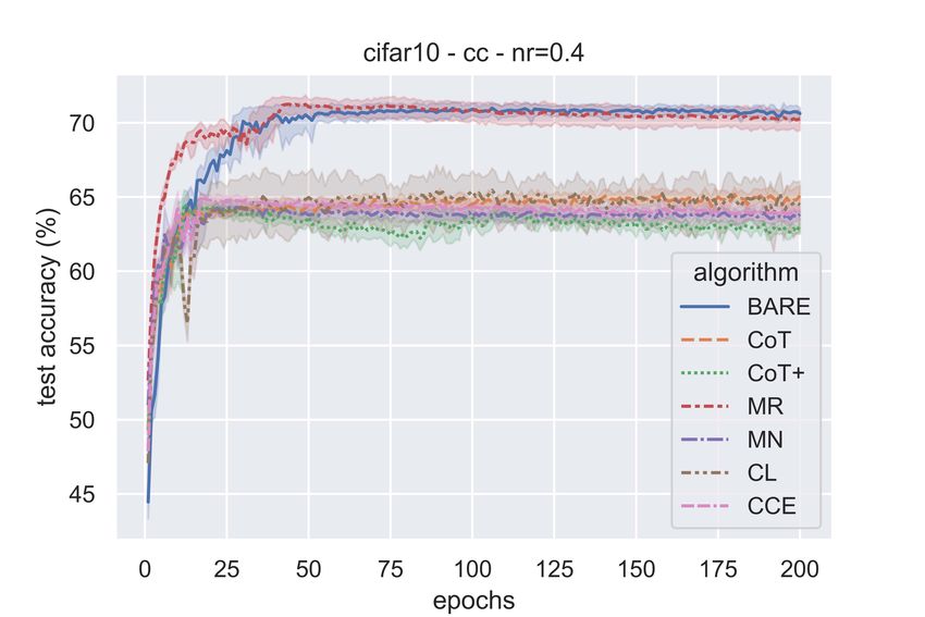
a similar idea. In all such approaches, the weight assigned to an example is essentially determined
by the loss function value on that example with a heuristic that, low loss values indicate reliable
labels. Many different ways of fixing/learning such weights have been proposed (e.g., [10, 31, 32]). A
good justification for this approach of assigning weights to examples for achieving robustness comes
from some recent studies on the effects of noisily-labelled data on learning deep neural networks.
It is empirically shown in [43] that deep neural networks can learn to achieve zero training error
on completely randomly labelled data, a phenomenon termed as ‘memorization’. However, further
studies such as [3, 23] have shown that the networks, when trained on randomly-labelled data, learn
simpler patterns (corresponding to cleanly-labelled data) first before overfitting to the noisily-labelled
data.
Motivated by this, several strategies of ‘curriculum learning’ have been devised that aim to select
(or give more weightage to) ‘clean’ samples for obtaining some degree of robustness against label
noise [8, 13, 21, 40, 42]. All such methods essentially employ the heuristic of ‘small loss’ for sample
selection or weighting wherein (a fraction of) small-loss valued samples are preferentially used for
learning the network. Algorithms such as Co-Teaching [8] and Co-Teaching+ [42] use two networks
and select samples with loss value below a threshold in one network to train the other. In Co-Teaching,
the threshold is chosen based on the knowledge of noise rates and is fixed throughout the training. The
same threshold is used in Co-Teaching+ but the sample selection is based on disagreement between
the two networks. The MentorNet [13], another recent algorithm based on curriculum learning, uses
an auxiliary neural network trained to serve as a sample selection function. There are other adaptive
sample reweighting schemes based on meta-learning such as [31, 32] which learn sample weights for
the examples.
Algorithms in [13, 32] use a separate network to learn a mapping from loss values to weights of
examples. Such methods need additional computing resources as well as access to extra data without
label noise and may need careful choice of hyperparameters. In addition, all such methods, in effect,
assume that one can assess whether or not an example has clean label based on some function of
the loss value of that example. However, loss value of any specific example is itself a function of
the current state of learning and it evolves with epochs. Loss values of even clean samples may
change over a significant range during the course of learning. Further, the loss values achievable by a
network even on clean samples may be different for examples of different classes. Other methods
based on curriculum learning such as [8, 42] use a threshold to pick up the examples with small loss
values in each mini-batch. This threshold is fixed using the noise rate which is not known and is often
difficult to estimate reliably. (As we show in this paper, the method is somewhat sensitive to errors in
estimated noise rate). While they adapt this threshold with epochs in a fixed manner, it is not really
dependent on the current state of learning.
Motivated by these considerations, we propose a simple, adaptive curriculum based selection strategy
called BAtch REweighting (BARE). The idea is to focus on the current state of learning, in a given
mini-batch, for identifying the noisily labelled data in it. The statistics of loss values of all examples
in a mini-batch would give useful information on current state of learning. Our algorithm utilizes
these batch statistics to compute the threshold for sample selection in a given mini-batch. This
will give us what is essentially a dynamic or adaptive curriculum where the selection of examples
is naturally tied to state of learning. For example, it is possible that the automatically calculated
threshold is different for different mini-batches even within the same epoch. Thus, our method uses a
dynamic threshold which naturally evolves as learning proceeds. In addition, while calculating the
batch statistics we take into consideration the class labels also and hence the dynamic thresholds are
also dependent on the given labels of the examples.
The main contribution of this paper is an adaptive sample selection strategy for robust learning that
is simple to implement, does not need any clean validation data, needs no knowledge at all of the
noise rates and also does not have any additional hyperparameters. We empirically demonstrate the
effectiveness of our algorithm on benchmark datasets: MNIST [18], CIFAR-10 [15], and Clothing-
1M [39] and show that our algorithm is much more efficient in terms of time and has as good or better
robustness compared to other algorithms for different types of label noise and noise rates.
The rest of the paper is organized as follows: Section 2 discusses related work, Section 3 discusses our
proposed algorithm. Section 4 discusses our empirical results and concluding remarks are provided
in Section 5.

                                                    2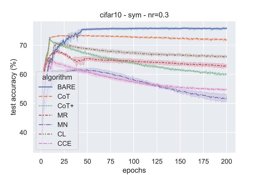
2    Related Work
Curriculum learning (CL) as proposed in [4] is the designing of an optimal sequence of training
samples to improve the model’s performance. The order of samples in this sequence is to be decided
based on a notion of easiness which can be fixed based on some prior knowledge. A curriculum called
Self-Paced Learning (SPL) is proposed in [17] wherein easiness is decided upon based on how small
the loss values are. A framework to unify CL and SPL is proposed in [12] by incorporating the prior
knowledge about curriculum and feedback from the model during training with the help of self-paced
functions that are to be used as regularizers. SPL with diversity [11] improved upon SPL by proposing
a sample selection scheme by encouraging selection of a diverse set of easy examples for learning
with the help of a group sparsity regularizer. This is further improved in [47] by encouraging more
exploration during early phases of learning.
Motivated by similar ideas, many sample reweighting algorithms are proposed for tackling label
noise in neural networks. Building on the empirical observations that the neural networks learn from
clean data first before overfitting to the noisy data, these methods attempt to reduce this gradual
overfitting by identifying the clean (easy) samples from the noisy (hard) samples with the help of
various heuristics. So, sample selection / reweighting algorithms for robust deep learning can be
viewed as designing a fixed or adaptive curriculum. A sample selection algorithm based on the
‘small loss’ heuristic wherein the algorithm will select a fraction of small loss valued samples for
training is proposed in [8, 42]. Two networks are cross-trained with samples selected by each other
based on this criterion. [21] also relies on ‘small loss’ heuristic but the threshold for sample selection
is adapted based on the knowledge of label noise rates. When a (small amount of) separate data
with clean labels is available, [13] proposes a data-dependent, adaptive curriculum learning method
wherein an auxiliary network trained on this clean data set is used to select reliable examples from
the noisy training data for training the classifier. When such clean data is not available, it reduces
to a non-adaptive, self-paced learning scheme. Another sample selection algorithm is proposed
in [25] where the idea is to train two networks and update the network parameters only in case of a
disagreement between the two networks. These sample selection functions are mostly hand-crafted
and, hence, they can be sub-optimal. A general strategy is to solve a bilevel optimization problem
to find the optimal sample weights. For instance, the sample selection function used in [8, 42] is
sub-optimally chosen for which [40] proposes an AutoML-based approach to find a better function,
by fine-tuning on separate data with clean labels. Sample reweighting algorithms proposed in [31]
and [32] use online meta-learning and need some extra data with clean labels. The method in [31]
uses the gradients of loss on noisy and clean data to learn the weights for samples while the method
in [32] tries to learn these weights as a function of their loss values.
Apart from the sample selection/reweighting approaches described above, there are other approaches
to tackling label noise. Label cleaning algorithms [33, 34, 41] attempt at identifying and correcting
the potentially incorrect labels through joint optimization of sample weights and network weights.
Loss correction methods [28, 36] suitably modify loss function (or posterior probabilities) to correct
for the effects of label noise on risk minimization; however, they need to know (or estimate) the noise
rates. There are also theoretical results that investigate robustness (to label noise) of risk minimization
under some special loss functions [7, 16, 22, 35, 45]. Regularization methods, of which sample
reweighting approaches are a part, employ explicit or implicit regularization to reduce overfitting to
noisy data [1, 19, 20, 24, 26, 30, 44]. In this paper our interest is in the approach of sample selection
for achieving robustness to label noise.
The BARE algorithm proposed here is a simple, adaptive curriculum to select samples which relies
only on statistics of loss values (or, equivalently, statistics of class posterior probabilities because
we use CCE loss) in a given mini-batch. We do not need any extra data with clean labels or any
knowledge about label noise rates. Since it uses batch statistics, the selection thresholds are naturally
tied to the evolving state of learning of the network without needing any tunable hyperparameters.
Unlike in many of the aforementioned algorithms, we do not need any auxiliary networks for learning
sample selection function, online reweighting or cross-training, or noise rate estimation and, thus, our
algorithm is computationally more efficient.

3    Batch Reweighting Algorithm
In this section we describe the proposed sample reweighting algorithm that relies on mini-batch
statistics.

                                                    3
3.1   Problem Formualtion and Notation

Under label noise, the labels provided in the training set may be ‘wrong’ and we want a classifier
whose test error with respect to ‘correct’ labels is good. We begin by making this more precise and
introducing our notation.
Consider a K-class problem with X as the feature/pattern space and Y = {0, 1}K as the label space.
We assume all labels are one-hot vectors and denote by ek the one-hot vector corresponding to class
k. Let S c = {(xi , yic ), i = 1, 2, · · · , m} be iid samples drawn according to a distribution D on
X × Y. Let us assume we are interested in learning a classifier that does well on a test set drawn
according to D. We can do so if we are given S c as training set. However, we do not have access to
this training set and what we have is a training set S = {(xi , yi ), i = 1, 2, · · · , m} drawn according
to a distribution Dη . The yi here are the ‘corrupted’ labels and they are related to yic , the ‘correct’
labels through
                                      P [yi = ek0 | yic = ek ] = ηkk0
The ηkk0 are called noise rates. (In general the above probability can depend on the feature vector,
xi , too though we do not consider that possibility in this paper). ηkk0 gives the probability of label k
getting changed into label k 0 . We call this general model as class conditional noise because here the
probability of label corruption depends on the original label. A special case of this is the so called
                                                                    η
symmetric noise where we assume ηkk = (1 − η) and ηkk0 = K−1           , ∀k 0 6= k. Here, η represents the
probability of a ‘wrong’ label. Symmetric noise corresponds to the case where the corrupted label is
equally likely to be any other label.
We can represent ηkk0 as a matrix and we assume it is diagonal dominant (that is, ηkk > ηkk0 , ∀k 0 6= k).
Note that this is true for symmetric noise if η < K−1    K . Under this condition, if we take all patterns
labelled by a specific class in the label-corrupted training set, then patterns that truly belong to that
specific class are still in majority in that set. (Note that, for a 10-class problem with symmetric noise,
this condition is satisfied if η < 0.9).
Now the problem of robust learning under label noise can be stated as follows: We want to learn a
classifier for the distribution D but given training data drawn from Dη .
We denote by f (·; θ) a classifier function parameterized by θ. We assume that the neural network
classifiers that we use have softmax output layer. Hence, while the training set labels, yi , are one-hot
vectors, we will have f (x; θ) ∈ ∆K−1 , where ∆K−1 ⊂ [0, 1]K is the probability simplex. We denote
by L(f (x; θ), y) the loss function used for the classifier training which in our case is the CCE loss.

3.2   Adaptive Curriculum through Batch Statistics

General curriculum learning can be viewed as minimization of a weighted loss [13, 17]:
                                                          m
                                                          X
                              min   Lwtd (θ, w)     =           wi L(f (xi ; θ), yi )
                         θ,w∈[0,1]m
                                                          i=1
                                                            +G(w) + β||θ||2
where G(w) represents the curriculum. Since one normally employs SGD for learning, we will
take m here to be the size of a mini-batch. One simple choice for the curriculum is [17] G(w) =
−λ||w||1 , λ > 0. Putting this in the above, omitting the regularization term and taking li =
L(f (xi ; θ), yi ), the optimization problem becomes
                                                    m
                                                    X
                        min     Lwtd (θ, w)    =          (wi li − λwi )
                     θ,w∈[0,1]m
                                                    i=1
                                                    Xm
                                               =          (wi li + (1 − wi )λ) − mλ
                                                    i=1

Under the usual assumption that loss function is non-negative, for the above problem, the optimal w
for any fixed θ is: wi = 1 if li < λ and wi = 0 otherwise. If we want an adaptive curriculum, we
want λ to be dynamically adjusted based on the current state of learning. First, let us consider the

                                                    4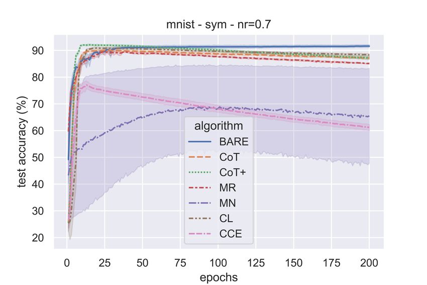
case where we make λ depend on the class label. The optimization problem becomes
                                                              m
                                                              X
                          min     Lwtd (θ, w)         =             (wi li − λ(yi )wi )
                       θ,w∈[0,1]m
                                                              i=1
                                                              K
                                                              X X
                                                      =                      (wi li − λj wi )
                                                              j=1 i:yi =ej
                                K
                                X X                                           K
                                                                              X X
                            =                  (wi li + (1 − wi )λj ) −                      λj
                                j=1 i:yi =ej                                  j=1 i:yi =ej

where λj = λ(ej ). As is easy to see, the optimal wi (for any fixed θ) are still given by the same
relation: for an i with yi = ej , wi = 1 when li < λj . Note that this relation for optimal wi is true
even if we make λj a function of θ and of all xi with yi = ej . Thus we can have a truly dynamically
adaptive curriculum by making these λj depend on all xi of that class in the mini-batch and the
current θ.
The above is an interesting theoretical insight: in the Self-Paced Learning formulation [17], the nature
of the final solution is same even if we make the λ parameter a function of the class-labels and also
other feature vectors corresponding to that class. This gives rise to class-label-dependent thresholds
on loss values. To the best of our knowledge, this direction of curriculum learning has not been
explored. It would be interesting to see how we can have curriculum designs that can exploit this.
Here, we are going to heuristically choose a function of class labels and feature vectors for λ.
So now the question is how we should choose these λj . As we mentioned earlier, we want these to be
determined by the statistics of loss values in the mini-batch.
Consider those i for which yi = ej . We would be setting wi = 1 and hence use this example to
update θ in this minibatch if this li < λj . We want λi to be fixed based on the observed loss values
of this mini-batch. Since there is sufficient empirical evidence that we tend to learn the clean samples
before overfitting to the noisy ones, some quantile or similar statistic of the set of observed loss values
in the mini-batch (among patterns labelled with a specific class) would be a good choice for λj .
Since we are using CCE loss, we have li = − ln (fj (xi ; θ)) and as the network has softmax output
layer, fj (xi ; θ) is the posterior probability of class-j under current θ for xi . Since the loss and this
posterior probability are inversely related, our criterion for selection of an example could be that the
assigned posterior probability is above a threshold which is some statistic of the observed posterior
probabilities in the mini-batch. In this paper we take the statistic to be mean plus one standard
deviation.
We can sum up the above discussion of our method of adaptive curriculum based on mini-batch
statistics as follows. In any mini-batch we set the weights for samples as

                                     1 if fyi (xi ; θ) ≥ λyi = µyi + σyi
                              wi =                                                                   (1)
                                     0 else
where µyi = |S1y | s∈Sy fyi (xs ; θ) and σy2i = |S1y | s∈Sy (fyi (xs ; θ)−µyi )2 indicate the sample
                     P                                  P
                   i        i                         i        i
mean and sample variance of the class posterior probabilities for samples having class label yi . [Note:
Syi = {k ∈ [m] | yk = yi } where m is the size of mini-batch]

Algorithm Implementation

Keeping in mind that neural networks are trained in a mini-batch manner, Algorithm 1 consists of
three parts: i.) computing sample selection thresholds, λyx , for a given mini-batch of data (Step 9-14),
ii.) sample selection based on these thresholds (Steps 16-20) as per Equation 1, and iii.) network
parameter updation using these selected samples (Step 21).

4   Experiments on Noisy Dataset
Dataset: We demonstrate the effectiveness of the proposed algorithm on two benchmark image
datasets: MNIST and CIFAR10. These data sets are used to benchmark almost all algorithms for

                                                          5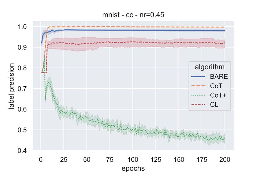
Algorithm 1 BAtch REweighting (BARE) Algorithm
 1: Input: noisy dataset Dη , # of classes K, # of epochs Tmax , learning rate α
 2: Initialize: Network parameters, θ0 , for classifier f (·; θ)
 3: for t = 0 to Tmax − 1 do
 4:   Shuffle the training dataset Dη
 5:   for i = 1 to |Dη |/|M| do
 6:      Draw a mini-batch M from Dη
 7:      m = |M| // mini-batch size
 8:      for p = 1 to K do
 9:         Sp = {k ∈P    [m] | yk = ep } // collect indices of samples with class-p
10:         µp = |S1p | s∈Sp fp (xs ; θt ) // mean posterior prob. for samples with class-p
            σp2 = |S1p | s∈Sp (fp (xs ; θt ) − µp )2 // variance in posterior prob. for samples with class-p
                        P
11:
12:         λp ← µp + σp // sample selection threshold for class-p as per Equation 1
13:      end for
14:      R ← φ // selected samples in M
15:      for each x ∈ M do
16:         if fyx (x; θt ) ≥ λyx then
17:            R ← R ∪ (x, yx ) // Select sample as per Equation 1
18:         end if
19:      end for
                               1
                                  P
20:      θt+1 = θt − α∇ |R|         (x,yx )∈R L(x, yx ; θt )         // parameter updates
21:   end for
22: end for
23: Output: θt

robust learning under label noise and we briefly describe the data sets. (The details of data sets are
given in Table 1). MNIST contains 60,000 training images and 10,000 test images (of size 28 × 28)
with 10 classes. CIFAR-10 contains 50,000 training images and 10,000 test images (of size 32 × 32)
with 10 classes.
We test the algorithms on two types of label noise: symmetric and class-conditional label noise. In
symmetric label noise, each label is randomly flipped to any of the remaining classes with equal
probability, whereas for class-conditional noise, label flipping is done in a set of similar classes.
For the simulations here, for MNIST, the following flipping is done: 1 ← 7, 2 → 7, 3 → 8, and
5 ↔ 6. Similarly, for CIFAR10, the following flipping is done: TRUCK → AUTOMOBILE, BIRD
→ AIRPLANE, DEER → HORSE, CAT ↔ DOG. We use this type of noise because that is arguably
a more realistic scenario and also because it is the type of noise, in addition to symmetric noise, that
other algorithms for learning under label noise have used. Apart from this, we also provide results
with an arbitrary nose rate matrix. For all the datasets, 80% of the training set is used for training and,
from the remaining 20% data, we sample 1000 images that constitute the validation set.
We also experiment with the Clothing-1M dataset [39] which is a large-scale dataset obtained
by scrapping off the web for different images related to clothing. It contains noise that can be
characterized as somewhat close to feature-dependent noise, the most generic kind of label noise.
An estimated 40% images have noisy labels. The training dataset contains 1 million images and the
number of classes are 14. There are additional training, validation, and test sets of 50k, 14k, and 10k
images respectively with clean labels. Since there’s a class imbalance, following similar procedure
as in existing baselines, we use 260k images from the original noisy training set for training while
ensuring equal number of images per class in the set and test set of 10k images for performance
evaluation.
Data Augmentations: For MNIST we use no data augmentation. For CIFAR-10 we do a random
cropping with padding of 4, and random horizontal flips. For Clothing-1M we do random cropping
while ensuring image size is fixed.
Baselines:We compare the proposed algorithm with the following algorithms from literature:

    (1.) Co-Teaching (CoT) [8] which involves cross-training of two similar networks by selecting a
         fraction (dependent on noise rates) of low loss valued samples;

                                                       6
Table 1: Dataset details
                                    TRAIN SIZE    TEST SIZE    # CLASS         SIZE

                   MNIST             60,000        10,000         10        28×28
                   CIFAR-10          50,000        10,000         10        32×32
                   C LOTHING -1M    10,00,000      10,000         14      224×224

      (2.) Co-Teaching+ (CoT+) [42] which improves upon CoT with the difference being sample
           selection only from the subset upon which the two networks’ predictions disagree;
      (3.) Meta-Ren (MR) [31], which involves meta-learning of sample weights on-the-fly by com-
           paring gradients for clean and noisy data;
      (4.) Meta-Net (MN) [32], which improves upon MR by explicitly learning sample weights via a
           separate neural network;
      (5.) Curriculum Loss (CL) [21], which involves a curriculum for sample selection based on
           (estimated) noise rates;
      (6.) Standard (CCE), which is the usual training through empirical risk minimization with
           cross-entropy loss (using the data with noisy labels).

Among these baselines, CoT, CoT+, and CL are sample selection algorithms that require knowledge
of noise rates. The algorithms CoT+ and CL need a few initial iterations without any sample selection
as a warm-up period; we used 5 epochs and 10 epochs as warm up period during training for MNIST
and CIFAR-10 respectively. MR and MN assume access to a small set of clean validation data.
Because of this, and for a fair comparison among all the baselines, a clean validation set of 1000
samples is used in case of MR and MN, and the same set of samples but with the noisy labels is used
for the rest of the algorithms including the proposed one.
Network architectures & Optimizers: While most algorithms for learning under label noise use
MNIST and CIFAR10 data, different algorithms use different network architectures. Here we have
decided to use small networks that give state of art performance on clean data and investigate the
robustness we get by using our algorithm. We use one MLP and one CNN architecture. For MNIST
we train a 1-hidden layer fully-connected network with Adam (learning rate = 2 × 10⁻⁴ and a learning
rate scheduler: ReduceLROnPlateau). (This is same as the network used for Co-Teaching and Co-
Teaching+ [8, 42]). For CIFAR-10 we train a 4-layer CNN with Adam [14] (learning rate = 2 × 10⁻³
and a learning rate scheduler: ReduceLROnPlateau). All networks are trained for 200 epochs. For
MR, SGD optimizer with momentum 0.9 and learning rate of 1 × 10⁻³ is used as the meta-optimizer.
For MN, SGD optimizer with learning rate of 2 × 10⁻³ is used as meta-optimizer. For CL, soft hinge
loss is used as suggested in [21] instead of cross-entropy loss. Rest of the algorithms implemented in
this chapter use cross-entropy loss. All the simulations are run for 5 trials. A pre-trained ResNet-50
is used for training on Clothing-1M with SGD (learning rate of 1 × 10⁻³ that is halved at epochs 6
and 11) with a weight decay of 1 × 10⁻³ and momentum 0.9 for 14 epochs. All experiments use
PyTorch [27], NumPy [9], scikit-learn [29], and NVIDIA Titan X Pascal GPU with CUDA 10.0.
Table 2 contains details about the network architecture used for training on MNIST and CIFAR-10
datasets. These settings of optimizer, learning rate, and learning rate scheduler were found to work
the best for our experimental and hardware setup. All the codes for these experiments are available
here: https://github.com/dbp1994/masters_thesis_codes/tree/main/BARE
Performance Metrics: For all algorithms we compare test accuracies on a separate test set with
clean labels. The main idea in all sample selection schemes is to identify noisy labels. Hence, in
addition to test accuracies, we also compare precision (# clean labels selected / # of selected labels)
and recall (# clean labels selected / # of clean labels in the data) in identifying noisy labels.

4.1     Discussion of Results

4.1.1    Performance on MNIST
Figure 1 shows the evolution of test accuracy (with training epochs) under symmetric (η ∈ {0.5, 0.7})
and class conditional (η = 0.45) label noise for different algorithms. We can see from the figure
that the proposed algorithm outperforms the baselines for symmetric noise. For the case of

                                                  7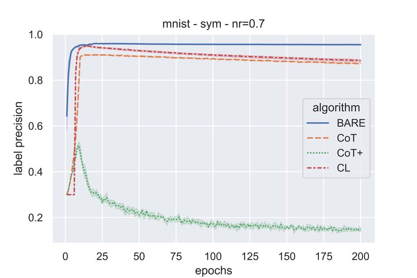
Table 2: Network Architectures used for training on MNIST and CIFAR-10 datasets
MNIST CIFAR-10
3×3 CONV., 64 R E LU, STRIDE 1, PADDING 1
BATCH N ORMALIZATION
2×2 M AX P OOLING , STRIDE 2
3×3 CONV., 128 R E LU, STRIDE 1, PADDING 1
BATCH N ORMALIZATION
DENSE 28×28 → 256 2×2 M AX P OOLING , STRIDE 2
3×3 CONV., 196 R E LU, STRIDE 1, PADDING 1
BATCH N ORMALIZATION
3×3 CONV., 16 R E LU, STRIDE 1, PADDING 1
BATCH N ORMALIZATION
2×2 M AX P OOLING , STRIDE 2
DENSE 256 → 10 DENSE 256 →10
(a) (b) (c)
Figure 1: Test Accuracies - MNIST - Symmetric (a & b) & Class-conditional (c) Label Noise
class-conditional noise, the test accuracy of the proposed algorithm is marginally less than the best of
the baselines, namely CoT and MR.
Figure 1 showed the evolution of test accuracies with epochs. We tabulate the final test accuracies
of all algorithms in Tables 3 – 5. The best two results are in bold. These are accuracies achieved at
the end of training. For CoT [8] and CoT+ [42], we show accuracies only of that network which
performs the best out of the two that are trained.
Table 3: Test Accuracy (%) for MNIST - η = 0.5 (symmetric)
A LGORITHM T EST ACCURACY
C OT [8] 90.80 ± 0.18
C OT+ [42] 93.17 ± 0.3
MR [31] 90.39 ± 0.07
MN [32] 74.94 ± 9.56
CL [21] 92.00 ± 0.26
CCE 74.30 ± 0.55
BARE (O URS ) 94.38 ± 0.13
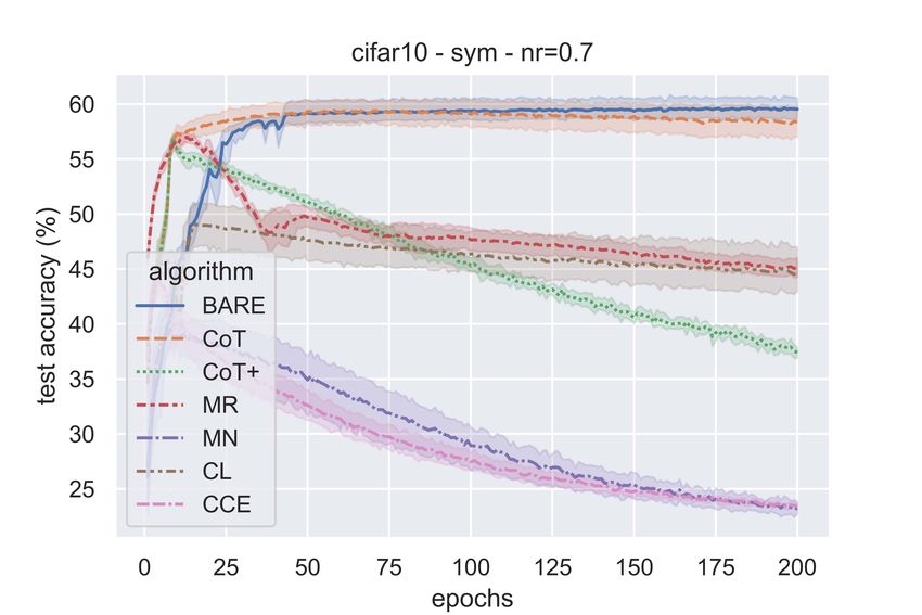
4.1.2 Performance on CIFAR-10
Figure 2 shows the test accuracies of the various algorithms as the training progresses for both
symmetric (η ∈ {0.3, 0.7}) and class-conditional (η = 0.4) label noise. We can see from the figure
that the proposed algorithm outperforms the baseline schemes and its test accuracies are uniformly
good for all types of label noise.
8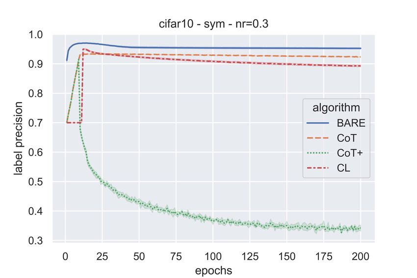
Table 4: Test Accuracy (%) for MNIST - η = 0.7 (symmetric)

                                 A LGORITHM        T EST ACCURACY
                                 C OT [8]              87.17 ± 0.45
                                 C OT+ [42]            87.26 ± 0.67
                                 MR [31]               85.10 ± 0.28
                                 MN [32]              65.52 ± 21.35
                                 CL [21]              88.28 ± 0.45
                                 CCE                   61.19 ± 1.29
                                 BARE (O URS )        91.61 ± 0.60

                Table 5: Test Accuracy (%) for MNIST - η = 0.45 (class-conditional)

                                 A LGORITHM        T EST ACCURACY
                                 C OT [8]             95.20 ± 0.22
                                 C OT+ [42]            91.10 ± 1.51
                                 MR [31]              95.40 ± 0.31
                                 MN [32]               75.03 ± 0.59
                                 CL [21]               81.52 ± 3.27
                                 CCE                   74.96 ± 0.21
                                 BARE (O URS )        94.11 ± 0.77

          (a)                                            (b)                                            (c)
  Figure 2: Test Accuracies - CIFAR10 - Symmetric (a & b) & Class-conditional (c) Label Noise

It is to be noted that while test accuracies for our algorithm stay saturated after attaining maximum
performance, the other algorithms’ performance seems to deteriorate as can be seen in the form of
accuracy dips towards the end of training. This suggests that our proposed algorithm doesn’t let the
network overfit even after long durations of training unlike the case with other algorithms.
All the algorithms, except the proposed one, have hyperparameters (in the sample selection/weighting
method) and the accuracies reported here are for the best possible hyperparameter values obtained
through tuning. The MR and MN algorithms are particularly sensitive to hyperparameter values in
the meta learning algorithm. In contrast, BARE has no hyperparameters for the sample selection and
hence no such tuning is involved.
As in the case of MNIST, we tabulate the final test accuracies of all algorithms on CIFAR in Tables 6
– 8. The best two results are in bold.
It may be noted from the tables giving test accuracies on MNIST and CIFAR-10, that sometimes the
standard deviation in the accuracy for MN is high. As we mentioned earlier, we noticed that MN
is very sensitive to the tuning of hyper parameters. While we tried our best to tune all the hyper
parameters, may be the final ones we found for these cases are still not the best and that is why the
standard deviation is high.

                                                  9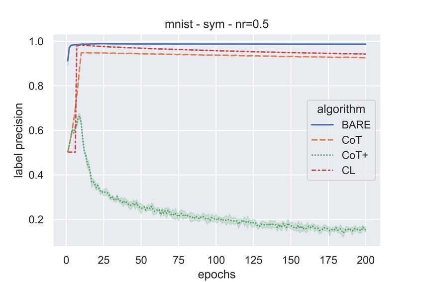
Table 6: Test Accuracy (%) for CIFAR-10 - η = 0.3 (symmetric)

                                 A LGORITHM        T EST ACCURACY
                                 C OT [8]             71.72 ± 0.30
                                 C OT+ [42]            60.14 ± 0.35
                                 MR [31]               62.96 ± 0.70
                                 MN [32]               51.65 ± 1.49
                                 CL [21]              66.124 ± 0.45
                                 CCE                   54.83 ± 0.28
                                 BARE (O URS )        75.85 ± 0.41

                 Table 7: Test Accuracy (%) for CIFAR-10 - η = 0.7 (symmetric)

                                 A LGORITHM        T EST ACCURACY
                                 C OT [8]             58.95 ± 1.31
                                 C OT+ [42]            37.69 ± 0.70
                                 MR [31]               45.14 ± 1.04
                                 MN [32]               23.23 ± 0.65
                                 CL [21]               44.82 ± 2.42
                                 CCE                   23.46 ± 0.37
                                 BARE (O URS )        59.53 ± 1.12

              Table 8: Test Accuracy (%) for CIFAR-10 - η = 0.4 (class-conditional)

                                 A LGORITHM        T EST ACCURACY
                                 C OT [8]              65.26 ± 0.78
                                 C OT+ [42]            63.05 ± 0.39
                                 MR [31]              70.27 ± 0.77
                                 MN [32]               63.84 ± 0.41
                                 CL [21]               64.48 ± 2.02
                                 CCE                   64.06 ± 0.32
                                 BARE (O URS )        70.63 ± 0.46

                       Table 9: Algorithm run times for training (in seconds)
                                A LGORITHM       MNIST     CIFAR10
                                BARE             310.64       930.78
                                C OT              504.5       1687.9
                                C OT+             537.7      1790.57
                                MR                807.4      8130.87
                                MN               1138.4       8891.6
                                CL               730.15       1254.3
                                CCE              229.27       825.68

4.1.3   Efficiency of BARE

Table 9 shows the typical run times for 200 epochs of training with all the algorithms. It can be seen
from the table that the proposed algorithm takes roughly the same time as the usual training with
CCE loss whereas all other baselines are significantly more expensive computationally. In case of
MR and MN, the run times are around 8 times that of the proposed algorithm for CIFAR-10.

                                                 10
4.1.4 Performance on Clothing1M
The results are summarized in Table 10. We report the baseline accuracies as observed in the
corresponding papers. And, for this reason, the baselines with which we compare our results are
different. These are the baselines that have reported results on this dataset. It shows that that even
for datasets used in practice which have label noise that isn’t synthetic unlike the symmetric and
class-conditional label noise used for aforementioned simulations, the proposed algorithm performs
better than all but one baselines. However, it is to be noted that DivideMix requires about 2.4
times the computation time required for BARE. In addition to this, DivideMix requires tuning of 5
hyperparameters whereas no such tuning is required for BARE.
Table 10: Test accuracies on Clothing-1M dataset
A LGORITHM T EST ACCURACY (%)
CCE 68.94
D2L [23] 69.47
GCE [45] 69.75
F ORWARD [28] 69.84
C OT [8]1 70.15
J O C O R [37] 70.30
SEAL [6] 70.63
DY [2] 71.00
SCE [35] 71.02
LRT [46] 71.74
PTD-R-V [38] 71.67
J OINT O PT. [34] 72.23
BARE (O URS ) 72.28
D IVIDE M IX [19] 74.76
(a) (b) (c)
Figure 3: Label Precision - MNIST - Symmetric (a & b) & Class-conditional (c) Label Noise
4.1.5 Efficacy of detecting clean samples
Figure 3 and Figure 4 show the label precision (across epochs) of the various algorithms on MNIST
and CIFAR-10 respectively. One can see from these figures that BARE has comparable or better
precision. Thus, compared to other sample selection algorithms, a somewhat higher fraction of
samples selected for training by BARE have clean labels. Figure 5 show the label recall values for
CoT, CoT+, CL, and BARE for MNIST (5(a)) and CIFAR-10 (5(b) & 5(c) ). It can be noted that
BARE consistently achieves better recall values compared to the baselines. Higher recall values
indicate that the algorithm is able to identify clean samples more reliably. This is useful, for example,
to employ a label cleaning algorithm on the samples flagged as noisy (i.e., not selected) by BARE.
CoT+ selects a fraction of samples where two networks disagree and, hence, after the first few epochs,
it selects very few samples (∼ 3000) in each epoch. Since these are samples in which the networks
disagree, a good fraction of them may have noisy labels. This may be the reason for the poor precision
1
as reported in [6]
11(a) (b) (c)
Figure 4: Label Precision - CIFAR10 - Symmetric (a & b) & Class-conditional (c) Label Noise
and recall values of CoT+ as seen in these figures. This can be seen from Figure 6 as well which
shows the fraction of samples chosen by the sample selection algorithms as epochs go by for MNIST
& CIFAR-10 dataset. It can be noted that, as noise rate is to be supplied to CoT and CL, they select
1 − η = 0.6 fraction of data with every epoch. Whereas, in case of CoT+, the samples where the
networks disagree is small because of the training dynamics and as a result, after a few epochs, it
consistently selects very few samples. Since the noise is class-conditional, even though η = 0.4, the
actual amount of label flipping is ∼ 20%. And this is why it’s interesting to note that BARE leads
to an approximate sample selection ratio of 80%. As is evident from these figures, BARE is able to
identify higher fraction of clean samples effectively even without the knowledge of noise rates.
(a) (b) (c)
Figure 5: Label Recall - Symmetric (a & b) & Class-conditional (c) Label Noise
(a) (b) (c)
Figure 6: (a): Sample fraction values for η = 0.5 (symmetric noise) on MNIST, (b): Sample
fraction values for η = 0.7 (symmetric noise) on CIFAR-10, (c): sample fraction values for η = 0.4
(class-conditional noise) on CIFAR-10
12(a) (b)
Figure 7: Test accuracies when estimated (symmetric) noise rate, η = 0.5, and true noise rate,
η = 0.7, for (a): MNIST & (b): CIFAR-10
While test accuracies and label precision values do demonstrate the effectiveness of algorithms for
this study, it’s also instructive and essential to look at the label recall values as one may want to know
if and when one needs to perform the tasks of cleaning/rectifying the noisy labels apart from sample
selection. Label recall also tells us how poorly a sample selection algorithm performs when it comes
to selecting reliable, clean samples. Figure 5 show the label recall values for CoT, CoT+, CL, and
BARE for MNIST and CIFAR10. It can be noted that the proposed algorithm consistently performs
better by exhibiting high recall values compared to the baselines.
4.1.6 Sensitivity to noise rates
Some of the baselines schemes such as CoT, CoT+, and CL require knowledge of true noise rates
beforehand. This information is typically unavailable in practice. One can estimate the noise rates
but there would be inevitable errors in estimation. Figure 7 shows the effect of mis-specification of
noise rates for these 3 baselines schemes. As can be seen from these figures, while the algorithms
can exhibit robust learning when the true noise rate is known, the performance deteriorates if the
estimated noise rate is erroneous. Obviously, BARE does not have this issue because it does not need
any information on noise rate.
4.1.7 Results on Arbitrary Noise Matrix
Earlier, we showed results for special cases of class-conditional noise. There the noise rate is still
specifiable by a single number and there is a pre-fixed pairs of classes that can be confused with
each other. As explained earlier, we have used this type of noise because that was what was used in
literature.
We now provide results for class-conditional noise with an arbitrary, diagonally-dominant noise
matrix. We show the noise matrices above. These noise matrices are chosen arbitrarily. However, as
can be seen, now in each row more than two entries can be non-zero.
The results obtained with different algorithms are shown in Tables 11–14. As mentioned earlier,
algorithms CoT, CoT+ and CL need knowledge of noise rate. With an arbitrary noise matrix, it is not
clear what number can be supplied as the noise rate for these algorithms, even if we know all the
noise rates. For these simulations, η = 0.45 and η = 0.4 are supplied as the estimated noise rates to
CoT, CoT+, and CL baselines for MNIST and CIFAR-10 respectively. In the tables, the best two
results are in bold. It can be seen that the proposed algorithm continues to perform well.
131 0 0 0 0 0 0 0 0 0
0 1 0 0 0 0 0 0 0 0
0 0 0.6 0 0 0 0 0.3 0 0.1
0 0 0 0.5 0 0.1 0 0 0.4 0
0 0 0 0 1 0 0 0 0 0
0 0 0 0 0.15 0.55 0.3 0 0 0
0 0 0 0 0 0.35 0.55 0.10 0 0
0 0.25 0 0 0 0 0 0.5 0 0.25
0 0 0 0 0 0 0 0 1 0
0 0 0 0 0 0 0 0 0 1
Arbitrary Noise Matrix for MNIST
1 0 0 0 0 0 0 0 0 0
0 1 0 0 0 0 0 0 0 0
0.2 0 0.7 0 0 0 0.1 0 0 0
0.1 0 0 0.6 0 0.1 0 0 0.2 0
0 0.1 0.1 0 0.7 0 0 0.1 0 0
0 0 0 0.1 0 0.6 0 0 0 0.3
0 0 0 0 0 0 1 0 0 0
0 0 0 0 0 0 0 1 0 0
0 0 0 0 0 0 0 0 1 0
0 0.1 0 0 0 0 0 0.1 0 0.8
Arbitrary Noise Matrix for CIFAR-10
Table 11: Test Accuracy (%) for MNIST - ηest = 0.45 (arbitrary noise matrix)
A LGORITHM T EST ACCURACY
C OT [8] 95.3
C OT+ [42] 93.07
CL [21] 88.41
BARE (O URS ) 95.02
Table 12: Avg. Test Accuracy (last 10 epochs) (%) for MNIST - ηest = 0.45 (arbitrary noise matrix)
A LGORITHM AVG . T EST ACCURACY ( LAST 10 EPOCHS )
C OT [8] 95.22
C OT+ [42] 93.08
CL [21] 88.56
BARE (O URS ) 95.03
Table 13: Test Accuracy (%) for CIFAR10 - ηest = 0.4 (arbitrary noise matrix)
A LGORITHM T EST ACCURACY
C OT [8] 71.92
C OT+ [42] 68.56
CL [21] 72.12
BARE (O URS ) 76.22
5 Conclusions
We propose an adaptive, data-dependent sample selection scheme, BARE, for robust learning in the
presence of label noise. The algorithm relies on statistics of assigned posterior probabilities of all
14Table 14: Avg. Test Accuracy (last 10 epochs) (%) for CIFAR10 - ηest = 0.4 (arbitrary noise matrix)
A LGORITHM AVG . T EST ACCURACY ( LAST 10 EPOCHS )
C OT [8] 71.86
C OT+ [42] 68.99
CL [21] 72.27
BARE (O URS ) 75.96
samples in a mini-batch to select samples from that minibatch. The mini-batch statistics are used as
proxies for determining current state of learning here. Unlike other algorithms in literature, BARE
neither needs an extra data set with clean labels nor does it need any knowledge of the noise rates.
Further it has no hyperparameters in the selection algorithm. Comparisons with baseline schemes on
benchmark datasets show the effectiveness of the proposed algorithm both in terms of performance
metrics and computational complexity.
The current algorithms for sample selection in literature rely on heuristics such as cross-training
multiple networks or meta-learning of sample weights which is often computationally expensive.
They also need knowledge of noise rates or some data with clean labels which may not be easily
available. From the results shown here, it seems that relying on the current state of learning via
batch statistics alone is helping the proposed algorithm confidently pick out the clean data and ignore
the noisy data (without even the need for cross training of two networks). This, combined with the
fact that there are no hyperparameters to tune, shows the advantage that BARE can offer for robust
learning under label noise.
Acknowledgements
We thank NVIDIA for providing us with NVIDIA Titan X Pascal & Maxwell GPUs.
References
[1] Eric Arazo, Diego Ortego, Paul Albert, Noel O’Connor, and Kevin McGuinness. Unsupervised label noise
modeling and loss correction. In International Conference on Machine Learning, pages 312–321. PMLR,
2019. 3
[2] Eric Arazo, Diego Ortego, Paul Albert, Noel O’Connor, and Kevin McGuinness. Unsupervised label noise
modeling and loss correction. In International Conference on Machine Learning, pages 312–321. PMLR,
2019. 11
[3] Devansh Arpit, Stanislaw Jastrzebski, Nicolas Ballas, David Krueger, Emmanuel Bengio, Maxinder S Kan-
wal, Tegan Maharaj, Asja Fischer, Aaron Courville, Yoshua Bengio, et al. A closer look at memorization
in deep networks. In International Conference on Machine Learning, pages 233–242. PMLR, 2017. 2
[4] Yoshua Bengio, Jérôme Louradour, Ronan Collobert, and Jason Weston. Curriculum learning. In
Proceedings of the 26th annual international conference on machine learning, pages 41–48, 2009. 1, 3
[5] Nontawat Charoenphakdee, Jongyeong Lee, and Masashi Sugiyama. On symmetric losses for learning
from corrupted labels. In International Conference on Machine Learning, pages 961–970. PMLR, 2019. 1
[6] Pengfei Chen, Junjie Ye, Guangyong Chen, Jingwei Zhao, and Pheng-Ann Heng. Beyond class-conditional
assumption: A primary attempt to combat instance-dependent label noise. arXiv preprint arXiv:2012.05458,
2020. 11
[7] Aritra Ghosh, Himanshu Kumar, and PS Sastry. Robust loss functions under label noise for deep neural
networks. In Proceedings of the Thirty-First AAAI Conference on Artificial Intelligence, pages 1919–1925,
2017. 1, 3
[8] Bo Han, Quanming Yao, Xingrui Yu, Gang Niu, Miao Xu, Weihua Hu, Ivor Tsang, and Masashi Sugiyama.
Co-teaching: Robust training of deep neural networks with extremely noisy labels. In Advances in neural
information processing systems, pages 8527–8537, 2018. 1, 2, 3, 6, 7, 8, 9, 10, 11, 14, 15
[9] Charles R Harris, K Jarrod Millman, Stéfan J van der Walt, Ralf Gommers, Pauli Virtanen, David
Cournapeau, Eric Wieser, Julian Taylor, Sebastian Berg, Nathaniel J Smith, Robert Kern, Matti Picus,
Stephan Hoyer, Marten H. van Kerkwijk, Matthew Brett, Allan Haldane, Jaime Fernández del Río,
Mark Wiebe, Pearu Peterson, Pierre Gérard-Marchant, Kevin Sheppard, Tyler Reddy, Warren Weckesser,
Hameer Abbasi, Christoph Gohlke, and Travis E. Oliphant. Array programming with NumPy. Nature,
585(7825):357–362, Sept. 2020. 7
15[10] Simon Jenni and Paolo Favaro. Deep bilevel learning. In Proceedings of the European conference on
computer vision (ECCV), pages 618–633, 2018. 2
[11] Lu Jiang, Deyu Meng, Shoou-I Yu, Zhenzhong Lan, Shiguang Shan, and Alexander Hauptmann. Self-paced
learning with diversity. In Advances in Neural Information Processing Systems, pages 2078–2086, 2014. 3
[12] Lu Jiang, Deyu Meng, Qian Zhao, Shiguang Shan, and Alexander Hauptmann. Self-paced curriculum
learning. In Proceedings of the AAAI Conference on Artificial Intelligence, volume 29, 2015. 3
[13] Lu Jiang, Zhengyuan Zhou, Thomas Leung, Li-Jia Li, and Li Fei-Fei. Mentornet: Learning data-driven
curriculum for very deep neural networks on corrupted labels. In International Conference on Machine
Learning, pages 2304–2313. PMLR, 2018. 1, 2, 3, 4
[14] Diederik P Kingma and Jimmy Ba. Adam: A method for stochastic optimization. arXiv preprint
arXiv:1412.6980, 2014. 7
[15] Alex Krizhevsky. Learning Multiple Layers of Features from Tiny Images. PhD thesis, University of
Toronto, 2009. 2
[16] H. Kumar and P. S. Sastry. Robust loss functions for learning multi-class classifiers. In 2018 IEEE
International Conference on Systems, Man, and Cybernetics (SMC), pages 687–692, 2018. 3
[17] M Pawan Kumar, Benjamin Packer, and Daphne Koller. Self-paced learning for latent variable models. In
Proceedings of the 23rd International Conference on Neural Information Processing Systems-Volume 1,
pages 1189–1197, 2010. 1, 3, 4, 5
[18] Yann LeCun, Léon Bottou, Yoshua Bengio, and Patrick Haffner. Gradient-based learning applied to
document recognition. Proceedings of the IEEE, 86(11):2278–2324, 1998. 2
[19] Junnan Li, Richard Socher, and Steven C.H. Hoi. Dividemix: Learning with noisy labels as semi-supervised
learning. In International Conference on Learning Representations, 2020. 3, 11
[20] Junnan Li, Yongkang Wong, Qi Zhao, and Mohan S Kankanhalli. Learning to learn from noisy labeled
data. In Proceedings of the IEEE/CVF Conference on Computer Vision and Pattern Recognition, pages
5051–5059, 2019. 1, 3
[21] Yueming Lyu and Ivor W. Tsang. Curriculum loss: Robust learning and generalization against label
corruption. In International Conference on Learning Representations, 2020. 2, 3, 7, 8, 9, 10, 14, 15
[22] Xingjun Ma, Hanxun Huang, Yisen Wang, Simone Romano, Sarah Erfani, and James Bailey. Normalized
loss functions for deep learning with noisy labels. In International Conference on Machine Learning,
pages 6543–6553. PMLR, 2020. 3
[23] Xingjun Ma, Yisen Wang, Michael E. Houle, Shuo Zhou, Sarah Erfani, Shutao Xia, Sudanthi Wijewick-
rema, and James Bailey. Dimensionality-driven learning with noisy labels. In Proceedings of the 35th
International Conference on Machine Learning, pages 3355–3364, 2018. 2, 11
[24] Xingjun Ma, Yisen Wang, Michael E Houle, Shuo Zhou, Sarah Erfani, Shutao Xia, Sudanthi Wijewickrema,
and James Bailey. Dimensionality-driven learning with noisy labels. In International Conference on
Machine Learning, pages 3355–3364. PMLR, 2018. 3
[25] Eran Malach and Shai Shalev-Shwartz. Decoupling" when to update" from" how to update". In Proceedings
of the 31st International Conference on Neural Information Processing Systems, pages 961–971, 2017. 3
[26] Takeru Miyato, Shin-ichi Maeda, Masanori Koyama, and Shin Ishii. Virtual adversarial training: a
regularization method for supervised and semi-supervised learning. IEEE transactions on pattern analysis
and machine intelligence, 41(8):1979–1993, 2018. 3
[27] Adam Paszke, Sam Gross, Francisco Massa, Adam Lerer, James Bradbury, Gregory Chanan, Trevor
Killeen, Zeming Lin, Natalia Gimelshein, Luca Antiga, Alban Desmaison, Andreas Kopf, Edward Yang,
Zachary DeVito, Martin Raison, Alykhan Tejani, Sasank Chilamkurthy, Benoit Steiner, Lu Fang, Junjie
Bai, and Soumith Chintala. Pytorch: An imperative style, high-performance deep learning library. In H.
Wallach, H. Larochelle, A. Beygelzimer, F. d'Alche-Buc, E. Fox, and R. Garnett, editors, Advances in
Neural Information Processing Systems 32, pages 8024–8035. Curran Associates, Inc., 2019. 7
[28] Giorgio Patrini, Alessandro Rozza, Aditya Krishna Menon, Richard Nock, and Lizhen Qu. Making deep
neural networks robust to label noise: A loss correction approach. In Proceedings of the IEEE Conference
on Computer Vision and Pattern Recognition (CVPR), July 2017. 1, 3, 11
[29] F. Pedregosa, G. Varoquaux, A. Gramfort, V. Michel, B. Thirion, O. Grisel, M. Blondel, P. Prettenhofer, R.
Weiss, V. Dubourg, J. Vanderplas, A. Passos, D. Cournapeau, M. Brucher, M. Perrot, and E. Duchesnay.
Scikit-learn: Machine learning in Python. Journal of Machine Learning Research, 12:2825–2830, 2011. 7
[30] Scott E Reed, Honglak Lee, Dragomir Anguelov, Christian Szegedy, Dumitru Erhan, and Andrew Rabi-
novich. Training deep neural networks on noisy labels with bootstrapping. In ICLR (Workshop), 2015.
3
[31] Mengye Ren, Wenyuan Zeng, Bin Yang, and Raquel Urtasun. Learning to reweight examples for robust
deep learning. In Proceedings of the 35th International Conference on Machine Learning, volume 80 of
Proceedings of Machine Learning Research, pages 4334–4343, 2018. 1, 2, 3, 7, 8, 9, 10
[32] Jun Shu, Qi Xie, Lixuan Yi, Qian Zhao, Sanping Zhou, Zongben Xu, and Deyu Meng. Meta-weight-net:
Learning an explicit mapping for sample weighting. In Advances in Neural Information Processing
Systems, pages 1919–1930, 2019. 1, 2, 3, 7, 8, 9, 10
16[33] Hwanjun Song, Minseok Kim, and Jae-Gil Lee. Selfie: Refurbishing unclean samples for robust deep
learning. In ICML, pages 5907–5915, 2019. 3
[34] Daiki Tanaka, Daiki Ikami, Toshihiko Yamasaki, and Kiyoharu Aizawa. Joint optimization framework
for learning with noisy labels. In Proceedings of the IEEE Conference on Computer Vision and Pattern
Recognition, pages 5552–5560, 2018. 1, 3, 11
[35] Yisen Wang, Xingjun Ma, Zaiyi Chen, Yuan Luo, Jinfeng Yi, and James Bailey. Symmetric cross entropy
for robust learning with noisy labels. In Proceedings of the IEEE/CVF International Conference on
Computer Vision, pages 322–330, 2019. 1, 3, 11
[36] Zhen Wang, Guosheng Hu, and Qinghua Hu. Training noise-robust deep neural networks via meta-
learning. In Proceedings of the IEEE/CVF Conference on Computer Vision and Pattern Recognition, pages
4524–4533, 2020. 1, 3
[37] Hongxin Wei, Lei Feng, Xiangyu Chen, and Bo An. Combating noisy labels by agreement: A joint training
method with co-regularization. 2020. 11
[38] Xiaobo Xia, Tongliang Liu, Bo Han, Nannan Wang, Mingming Gong, Haifeng Liu, Gang Niu, Dacheng
Tao, and Masashi Sugiyama. Part-dependent label noise: Towards instance-dependent label noise. Advances
in Neural Information Processing Systems, 33, 2020. 11
[39] Tong Xiao, Tian Xia, Yi Yang, Chang Huang, and Xiaogang Wang. Learning from massive noisy labeled
data for image classification. In Proceedings of the IEEE conference on computer vision and pattern
recognition, pages 2691–2699, 2015. 2, 6
[40] Quanming Yao, Hansi Yang, Bo Han, Gang Niu, and James Tin-Yau Kwok. Searching to exploit
memorization effect in learning with noisy labels. In Proceedings of the 37th International Conference
on Machine Learning, volume 119 of Proceedings of Machine Learning Research, pages 10789–10798.
PMLR, 2020. 2, 3
[41] Kun Yi and Jianxin Wu. Probabilistic end-to-end noise correction for learning with noisy labels. In
Proceedings of the IEEE/CVF Conference on Computer Vision and Pattern Recognition, pages 7017–7025,
2019. 3
[42] Xingrui Yu, Bo Han, Jiangchao Yao, Gang Niu, Ivor Tsang, and Masashi Sugiyama. How does disagreement
help generalization against label corruption? In Proceedings of the 36th International Conference on
Machine Learning, pages 7164–7173, 2019. 2, 3, 7, 8, 9, 10, 14, 15
[43] Chiyuan Zhang, Samy Bengio, Moritz Hardt, Benjamin Recht, and Oriol Vinyals. Understanding deep
learning requires rethinking generalization. arXiv preprint arXiv:1611.03530, 2016. 2
[44] Hongyi Zhang, Moustapha Cisse, Yann N Dauphin, and David Lopez-Paz. mixup: Beyond empirical risk
minimization. arXiv preprint arXiv:1710.09412, 2017. 3
[45] Zhilu Zhang and Mert R Sabuncu. Generalized cross entropy loss for training deep neural networks with
noisy labels. arXiv preprint arXiv:1805.07836, 2018. 1, 3, 11
[46] Songzhu Zheng, Pengxiang Wu, Aman Goswami, Mayank Goswami, Dimitris Metaxas, and Chao Chen.
Error-bounded correction of noisy labels. In International Conference on Machine Learning, pages
11447–11457. PMLR, 2020. 11
[47] Tianyi Zhou and Jeff Bilmes. Minimax curriculum learning: Machine teaching with desirable difficulties
and scheduled diversity. In International Conference on Learning Representations, 2018. 3
17A Appendix
Performance of BARE on low noise rates
As we can see in Table 15, the performance of BARE is good even when the noise rates are very low.
That’s why we don’t show these numbers in the paper when noise rate is low.
Table 15: Test accuracies for BARE on MNIST & CIFAR-10
DATASET N OISE R ATE T EST ACCURACY (%)
MNIST 0% 96.93 (±0.19)
MNIST 10% ( SYM .) 96.68 (±0.15)
MNIST 20% ( SYM .) 96.1 (±0.25)
CIFAR-10 0% 79.59 (±0.38)
CIFAR-10 10% ( SYM .) 78.76 (±0.43%)
CIFAR-10 20% ( SYM .) 77.04 (±0.61%)
Architectures and Performance
We have either used the same or very similar architectures as the ones used in Co-Teaching and
Co-Teaching+ papers for a fairer comparison.
Since the proposed method is a sample selection algorithm, we provided the precision and recall
curves which very clearly show the advantages and effectiveness of BARE in picking training
examples with clean labels. Since BARE is a sample selection algorithm, we compare against
state-of-art sample reweighting algorithms. Our algorithm offers advantages such as efficiency in
computation and higher label precision and recall indicating that the method is indeed more attractive
than the baselines.
Since different papers in literature use different architectures and different tuning of learning, we
cannot directly compare raw accuracies.
Table 10 shows that even for bigger architectures the advantages of the algorithm hold.
Relationship between loss values, `j , and sample selection threshold λj
We are motivated by an interesting theoretical insight: in the Self-Paced-Learning (optimization)
formulation, the nature of the final solution is same even if we make the λ parameter a function
of class-label and also other feature vectors of that class; this gives rise to class-label-dependent
thresholds on loss values. To the best of our knowledge, this direction of curriculum learning that
we pointed out has not been explored. And, in this work, we suggest a heuristic method to use this
flexibility.
Does the proposed algorithm have no hyperparameters?
In the proposed algorithm, there are no additional hyperparameters to tune. Even while learning
with no label noise, mini-batch size, learning-step-size, regularization, etc. are all hyperprameters
that need to be tuned. Our sample selection method does not have any new hyperparameters to be
tuned.
Sensitivity to Batch Size
To show the insensitivity to batch size, we show in Table 16 results on MNIST & CIFAR-10 for both
types of label noise and three batch sizes: 64, 128 (used in paper), & 256.
The case of large number of classes
With large number of classes, the number of samples of a given class in a mini-batch may be small.
One way of tackling it is to make mini-batches so that each mini-batch contains samples only from,
18You can also read