D3.11 Big Data Toolbox Training Manual II - Parsec Accelerator
←
→
Page content transcription
If your browser does not render page correctly, please read the page content below
D3.11 Big Data Toolbox Training
           Manual II
   WP3 – Large Scale Demonstrators

       Authors: Dimitar Misev, Peter Baumann
                       Date: 28.07.20

   This project has received funding from the European Union’s Horizon 2020
   research and innovation programme under grant agreement No 824478.
D3.11 Big Data Toolbox Training Manual II

Full Title            Promoting the international competitiveness of European Remote Sensing
                      companies through cross-cluster collaboration
Grant Agreement No 824478                         Acronym                  PARSEC

Start date            1st May 2019                Duration                 30 months

EU Project Officer    Milena Stoyanova

Project Coordinator   Emmanuel Pajot (EARSC)

Date of Delivery      Contractual         31.07.2020         Actual             28.07.2020

Nature                Report                      Dissemination Level      Public

Lead Beneficiary      RASDAMAN

Lead Author           Dimitar Misev               Email                    misev@rasdaman.com

Other authors         Peter Baumann (RASDAMAN), Gedas Vaitkus (GEOMATRIX)

Reviewer(s)           Weronika Borejko (EARSC)

Keywords              big data, EO, datacubes, array databases, OGC services, rasdaman

Document History
Version    Issue date      Stage           Changes                            Contributor
1.0        29.06.2020      Draft           First draft                        RASDAMAN
1.1        28.07.2020      Draft           Integrate GMX contributions        GEOMATRIX
1.2        28.07.2020      Final           Integrate review comments          RASDAMAN,
                                                                              EARSC

Disclaimer
Any dissemination of results reflects only the author’s view and the European Commission is not
responsible for any use that may be made of the information it contains

Copyright message
© PARSEC consortium, 2019
This deliverable contains original unpublished work except where clearly indicated otherwise.
Acknowledgment of previously published material and of the work of others has been made
through appropriate citation, quotation or both. Reproduction is authorised provided the source
is acknowledged.

                                                                                         Page 2 of 43
D3.11 Big Data Toolbox Training Manual II

Table of Contents
List of Acronyms ....................................................................................................................................... 5
Executive Summary .................................................................................................................................. 6
1.     Introduction ..................................................................................................................................... 7
2.     Available Datacubes ......................................................................................................................... 7
     2.1      Sentinel-1 ................................................................................................................................. 7
       2.1.1          Global datacubes with on-demand pre-processing ......................................................... 7
       2.1.2          Local pre-processed datacubes ........................................................................................ 8
       2.1.3          Local pre-processed datacubes with user-defined area of interest ................................ 9
     2.2      Sentinel-2 ............................................................................................................................... 15
       2.2.1          Level-1C .......................................................................................................................... 15
       2.2.2          Level-2A.......................................................................................................................... 15
     2.3      Sentinel-5p ............................................................................................................................. 15
     2.4      EU-DEM .................................................................................................................................. 17
3.     Datacube Download with WCS ...................................................................................................... 17
     3.1      Core ........................................................................................................................................ 18
     3.2      Updating ................................................................................................................................. 19
     3.3      Processing .............................................................................................................................. 19
     3.4      Range subsetting .................................................................................................................... 19
     3.5      Scaling .................................................................................................................................... 19
     3.6      Reprojection ........................................................................................................................... 20
     3.7      Interpolation .......................................................................................................................... 20
4.     Datacube Analytics with WCPS ...................................................................................................... 21
     4.1      Scalar operations ................................................................................................................... 21
     4.2      Coverage operations .............................................................................................................. 22
     4.3      Metadata operations ............................................................................................................. 23
     4.4      BigDataToolbox Examples ...................................................................................................... 23
       4.4.1          True color composite ..................................................................................................... 24
       4.4.2          False color composite .................................................................................................... 24
       4.4.3          Normalized Difference Vegetation Index (NDVI) ........................................................... 25
       4.4.4          Data fusion ..................................................................................................................... 26
       4.4.5          Polygon clipping ............................................................................................................. 27
       4.4.6          Aggregation .................................................................................................................... 27
       4.4.7          Map coloring .................................................................................................................. 27

                                                                                                                                          Page 3 of 43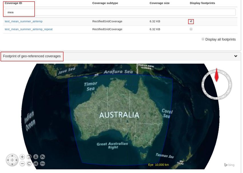
D3.11 Big Data Toolbox Training Manual II

5.     Datacube Portrayal with WMS ...................................................................................................... 29
6.     Clients............................................................................................................................................. 30
     6.1      Rasdaman WSClient ............................................................................................................... 30
       6.1.1          WCS ................................................................................................................................ 30
       6.1.2          WMS ............................................................................................................................... 35
     6.2      Python / Jupyter Notebook .................................................................................................... 38
     6.3      NASA WebWorldWind ........................................................................................................... 39
     6.4      OpenLayers ............................................................................................................................ 40
     6.5      Leaflet .................................................................................................................................... 40
     6.6      QGIS ....................................................................................................................................... 41
     6.7      Command-line tools ............................................................................................................... 41
7.     Additional Resources ..................................................................................................................... 42

Table of Figures
Figure 1 True color composite query result ........................................................................................... 24
Figure 2 False color query result ............................................................................................................ 25
Figure 3 NDVI query result ..................................................................................................................... 26
Figure 4 Data combination query result ................................................................................................ 26
Figure 5 Polygon clipping query result ................................................................................................... 27
Figure 6 DEM map coloring query result ............................................................................................... 28
Figure 7 WMS demo screenshot ............................................................................................................ 29
Figure 8 List of coverages shown on the GetCapabilities tab. ............................................................... 30
Figure 9 Selected coverage footprints shown on a globe. ..................................................................... 31
Figure 10 WCS service metadata. .......................................................................................................... 31
Figure 11 Showing full description of a coverage. ................................................................................. 32
Figure 12 Updating the metadata of a coverage. .................................................................................. 32
Figure 13 Downloading a subset of a coverage, encoded in image/tiff. ............................................... 33
Figure 14 Query and output areas on the ProcessCoverages tab. ........................................................ 34
Figure 15 Deleting coverage test_DaysPerMonth. ................................................................................ 34
Figure 16 Inserting a coverage given a URL pointing to a valid GML document. .................................. 34
Figure 17 List of layers shown on the GetCapabilities tab. .................................................................... 35
Figure 18 Selected layer footprints shown on a globe. ......................................................................... 36
Figure 19 Showing full description of a layer. ........................................................................................ 36
Figure 20 Showing/hiding a layer on the map. ...................................................................................... 37
Figure 21 Style management on the DescribeLayer tab. ....................................................................... 38

Table of Tables
Table 1 Sentinel -5p product sand variables .......................................................................................... 17
Table 2. Standard operations returning scalar values. .......................................................................... 22
Table 3. Aggregation operations. ........................................................................................................... 22
Table 4. Metadata operations. .............................................................................................................. 23

                                                                                                                                          Page 4 of 43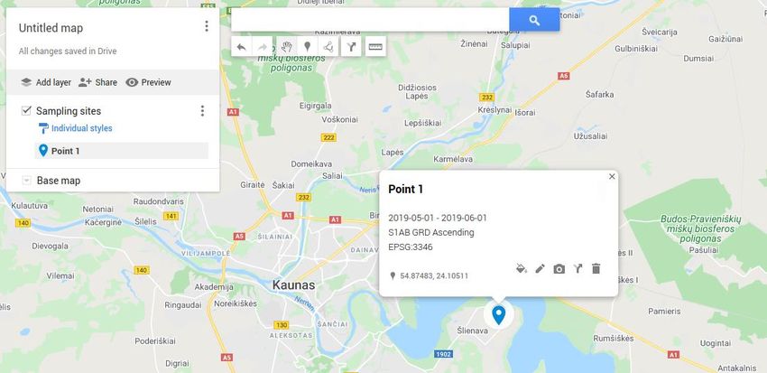
D3.11 Big Data Toolbox Training Manual II

List of Acronyms
API    Application Programming Interface
CRS    Coordinate Reference System
EO     Earth Observation
GRD    Sentinel-1 product type, Ground Range Detected
OGC    Open Geospatial Consortium
SLC    Sentinel-1 product type, Single Look Complex
WMS    Web Map Service
WCPS   Web Coverage Processing Service
WCS    Web Coverage Service

                                                                 Page 5 of 43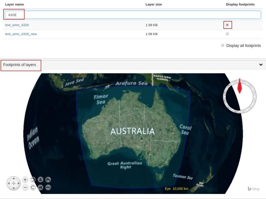
D3.11 Big Data Toolbox Training Manual II

Executive Summary
This document is a companion training manual for the Big Data Toolbox service offered by PARSEC.
The public user-facing interfaces and API of the Big Data Toolbox are comprised of standard OGC
services for big EO datacubes:

   •   WCS for downloading datacubes in desired projection and format, with flexible spatio-
       temporal and range subsetting applied as needed;
   •   WCPS for doing filtering, processing, and analytics on datacubes through a powerful but
       concise and safe declarative query language;
   •   WMS for visualizing and exploring datacubes, usually as maps in the browser.

The training manual aims to be pragmatic in style and focuses on serving as a concise introduction to
these standard interfaces, with simple practical examples to aid quick understanding. As the Big Data
Toolbox service is powered by a rasdaman server on the backend, the documentation and mailing
lists of rasdaman can be considered as additional resources for more advanced topics not explicitly
covered in this document. Additionally, the standard documents published by OGC are useful as
canonical references.

                                                                                        Page 6 of 43
D3.11 Big Data Toolbox Training Manual II

1. Introduction
The PARSEC Big Data Toolbox service offers access to large EO data (Section 2) via standard OGC
interfaces:

    •   WCS for data subsetting and download (Section 3)
    •   WCPS for big data processing and analytics (Section 4)
    •   WMS for visualizing and exploring datacube maps (Section 5)

These API are accessible through a variety of client tools and libraries (Section 6).

This document is a training manual for the Big Data Toolbox which aims to be pragmatic in style with
simple practical examples to aid quick understanding. It is mainly aimed at developers of more
specialized and user-friendly tools or services that build on top of the EO data offered by the Big Data
Toolbox. This encompasses all PARSEC beneficiaries that work with big EO datacubes.

This training manual is self-contained and can be followed in isolation. As the Big Data Toolbox
service is powered by a rasdaman server on the backend, the documentation and mailing lists of
rasdaman can be considered as additional resources for more advanced topics not explicitly covered
in this document. Additionally, the standard documents published by OGC are useful as canonical
references.

2. Available Datacubes
This Section lists the datacubes offered by the BigDataToolbox. Each of these datacubes can be
accessed for download (Section 2.4), processing and analytics (Section 4), and visualization as maps
(Section 5).

 2.1 Sentinel-1
 2.1.1 Global datacubes                                  with          on-demand                pre-
       processing
Sentinel-1 generally requires time-consuming pre-processing in order to build an analysis-ready data
cube out of it, as well as expensive disk storage. However, for the Big Data Toolbox rasdaman
managed to establish a datacube building procedure that allows to shift the time-consuming pre-
processing to an on-the-fly calculation happening during the data retrieval stage when users make
queries to the system. This enabled registering and offering Petabytes of Sentinel-1 data through the
Big Data Toolbox with only a small penalty of slower data access (less than one minute per one whole
scene). As the data is registered and loaded on demand from the DIAS online S3 storage, the
datacube could be established with minimal local disk space usage of around 0.5 TB, similar as in the
case of Sentinel-2 datacubes.

Datacube details:
                                                                                           Page 7 of 43
D3.11 Big Data Toolbox Training Manual II

    •   Temporal extent: 2018-01-01 - 2020-06-30
    •   Spatial extent: global
    •   Coordinate Reference System: EPSG:4326
    •   Naming scheme: S1_${product}_${modebeam}_${polarisation}, e.g. S1_GRD_IW_VV
            o ${product} - GRD or SLC
            o ${modebeam} - IW, EW, WV, S1, S2, S3, S4, S5, or S6
            o ${polarisations} - VV, VH, HH, or HV

 2.1.2 Local pre-processed datacubes
Several spatio-temporal areas have been pre-processed in order to allow real-time datacube access.
They are offered on the SAGRIS datacube at http://parsec.landimage.info/rasdaman/ows and are
arranged into several coverages for separate countries. This datacube is federated with the main
DIAS service, and hence the data is available through both endpoints.
Datacube naming conventions follow the same structure, e.g. S1_GRD_VH_SAGRIS_LIT_3346_10m,
where
    • S1 indicates satellite sensor
    • GRD – product processing level
    • VH/VV – product thematic content
    • SAGRIS – pre-processing work-flow (also specification)
    • LIT – reference country/region
    • 3346 – EPSG code of the pre-processed data loaded into rasdaman database
    • 10m – spatial resolution of raster products.

Full list of available datacubes:

    •   Lithuania – temporal extent: full Sentinel-1 time series covering 2015-03-02 – 2020-07-08,
        spatial extent – whole country, time series – all GRD(H) VV and VH images. This dataset is
        provided for:
        ◦ Monitoring the environment changes and climate impacts during a wide range of
            conditions, including normal seasons, extreme droughts and floods, normal, cold and
            mild winters, spring floods, etc.;
        ◦ Analysis of the land cover change and mapping of land use intensity – detection of
            permanent grassland, development of transitional woodland, etc.
        ◦ Detection of crops and monitoring crop development;
        ◦ Development and testing of forestry applications.

    •   Latvia – temporal extent: 2019-02-25 – 2019-07-05, spatial extent – whole country, time
        series – all GRD(H) VV and VH images. This dataset is provided for:
        ◦ Development and testing of forestry applications and sustainable energy (bio-fuel);
        ◦ Development and testing of trans-boundary applications and services in the fields of
            environment and agriculture;
        ◦ Monitoring of physical (moisture/drought) conditions in coastal and inland wetlands of
            the northern Europe;
        ◦ Monitoring the environment changes in semi-natural landscape used for extensive
            agriculture (cattle grazing in particular).

    •   Denmark – temporal extent: 2019-05-01 – 2019-08-29, spatial extent – whole country, time
        series – all GRD(H) VV and VH images. This dataset is provided for:

                                                                                      Page 8 of 43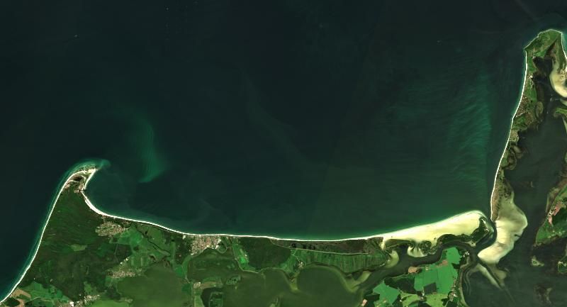
D3.11 Big Data Toolbox Training Manual II

        ◦   Monitoring the environment changes in northern Europe grasslands and coastal
            ecosystems affected by tides;
        ◦   Crop detection and monitoring of hazardous weather impacts on crops cultivated in mild
            winter conditions;
        ◦   Detection of ships in coastal waters.

    •   Azerbaijan – temporal extent: 2019-03-01 – 2019-07-04, spatial extent – whole country, time
        series – all GRD(H) VV and VH images. This dataset is provided for:
        ◦ Monitoring the environment changes in large coastal and inland wetland ecosystems;
        ◦ Monitoring seasonal dynamics in agriculture production of mountain regions;
        ◦ Detection of coastal and off-shore oil spills;

    •   Uzbekistan – temporal extent: 2018-03-01 – 2018-11-03, spatial extent – whole country, time
        series – all GRD(H) VV and VH images. This dataset is provided for:
        ◦ Analysis of large-scale desertification processes;
        ◦ Monitoring seasonal dynamics of water resources in Central Asia rivers;
        ◦ Testing crop detection and smart farming algorithms in irrigated farmland systems with
            two harvests per season.

    •   Spain – spatial extent: Madrid, Lat[40.0823, 40.6848] and Long[-4.3341, -3.2574] (EPSG:4326)

2.1.3 Local pre-processed datacubes with user-defined
      area of interest
SAGRIS tasking for Sentinel-1 polSAR data pre-processing is based on a concept of automated
discovery, download and processing of the whole satellite data time series based on a user-defined
period and region (or location) without manual browsing and selection from image catalog. This
concept is different from that of Sentinel products available on on DIAS portals, where users have to
manually pick up cloud-free images by searching and browsing the on-line catalog using a web
interface.

Following SAGRIS automated processing concept, Sentinel-1 discovery, download and processing is
routinely tasked by programming daily processing batches with automated and self-activating scripts.
SAGRIS clients need to provide a bounding polygons, indicate sampling periods and EPSG projection
codes on a simple yet comfortable web interface, implemented on the basis of Google My Maps
service.

Placing orders for Sentinel-1 pre-processing on SAGRIS service can be done by completing the
following simple steps:

1. Sign into your Google account by opening your mailbox at http://mail.google.com. If you do not
have a Google account yet, it is necessary to create a new one for managing your SAGRIS processing
orders. If you have not connected to your Google account before proceeding to the next step, you
will be automatically requested to do so while opening Your Maps section, as described in step 2 of
the current manual.

                                                                                        Page 9 of 43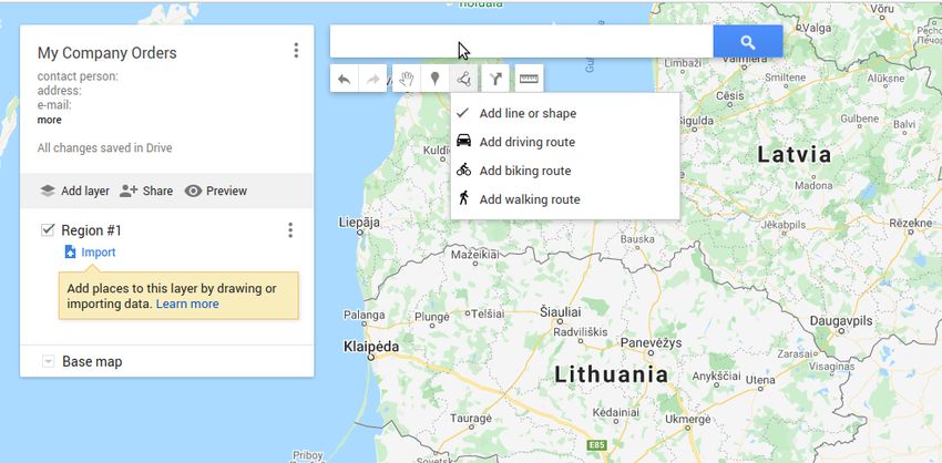
D3.11 Big Data Toolbox Training Manual II

Obligatory requirement to use Google account for SAGRIS tasking may seem not convenient for some
users, however exploitation of Google services offer a number of very useful functions, like safe login,
e-mail communication and sharing of processing orders, as well as on-line archive of editable and
shareable SAGRIS processing orders, which can be easily accessed by both client and service
operators, providing an on-line collaboration platform for both parties to update and finalize the
processing request, also on demand delivery processing results in the form of files.

2. Open Your Maps section at https://www.google.com/maps/d/home?hl=en and click on [CREATE
A NEW MAP] button if this is the first time you are using Google Your Maps service to place a SAGRIS
image processing order. If you want to update and re-submit map(-s) with processing orders created
and saved earlier, please click on a selected map on Your Maps entry screen.

                                                                                          Page 10 of 43
D3.11 Big Data Toolbox Training Manual II
3. To create a new processing order, the users will first of all have to fill-in the processing order
attribute details on the map project window on the top-left part of the map screen. This section will
must importantly have contact information of the client, as well as arrangement and naming of the
requested processing areas, represented as map layers:
The main window of your orders map can be used
to insert, edit and delete the regions (polygons)
ordered for processing, as well as their technical
details (period, sensors, orbits and projections). The
main window must contain the essential contact
information (company, address, e-mail, phone and
name of the contact person) related to processing
order. Clicking on three dots button in the top right
corner of this section will open a map management
menu with essential tasks, including export of the
order as KML/KMZ file with boundaries and
technical details of all polygons.
By pressing [Add layer] button in the middle of the map management window, the user can insert
new regions or “projects”, which can have several polygons, each specifying different sampling
periods, projections, etc.
Page 11 of 43D3.11 Big Data Toolbox Training Manual II
4. After completing the contact details of the processing order, the clients sill have to zoom into their
region of interest, click [Draw a line] button, select [Add line or shape] option
from drop-down menu and manually digitize a
bounding polygon of the area ordered for
processing. Completing the polygon is done by
merging its last node to the first one. After the
polygon is closed by merging the nodes, the
pop-up window will show up for the users to
fill in the essential order information,
associated with the current polygon.
It is important to note that all Sentinel images which overlap with the delineated polygon will be
selected for processing, therefore much larger are will be covered by Sentinel images than the
digitized polygon is actually covering. To reduce the number of images tasked for processing, we
recommend to delineate slightly smaller boundary than the actual area of interest, or indicate only
Ascending (or Descending) orbits.
Page 12 of 43D3.11 Big Data Toolbox Training Manual II
The user is requested to type in the following information in the attribute pop-up window, associated
with each manually digitized polygon or point used by the clients for area- or site-based SAGRIS
production tasking:
• Requested start and stop dates of the sampling period (mandatory);
• Requested sensor (Sentinel-1 A or B or AB), product type;
• Requested product. The only available option currently is Interferometric Wide Swath (IW)
Ground Range Detected (GRD) SAR products, so this information can be omitted;
• Requested orbits information – Ascending (A) or Descending (D) or both AD. If omitted, both
A and D orbits will be processed;
• Requested projection to be used for processing, which must be provided as a standard EPSG
code. If this parameter is omitted, a standard geographic coordinate system will be used for
processing.
Page 13 of 43D3.11 Big Data Toolbox Training Manual II
Digitizing one point as location for tasking a Sentinel-1 time series sampling is even more simple. This
can be done by clicking [Add marker] button on the main menu. After placing a marker, the attribute
pop-up window will appear. Attribute data must be typed in the same way as it is requested for the
polygon sampling area. It is also possible to drag the marker into a different position.
5. As mentioned earlier, attribute information and
area boundaries or points locations can be edited
and updated at any time. After each update the
maps should be delivered to the service
management team by re-sharing the saved My
Maps project. The team will revise the orders and
confirm tasking or request to provide additional
details.
By placing the processing order with Google My Maps, the users will provide the essential metadata
and geo-location information in a standard XML notation of a Google KML file format:
Polygon #1
S1AB GRDH A+DEPSG:3346]]>
#poly-000000-1200-77
1
20.8006948,56.0917871,0
20.5041244,55.2494833,0
22.5029931,54.8341334,0
22.5359337,54.388911,0
23.326701,53.8481895,0
24.3481211,53.7898352,0
25.9077033,54.1065595,0
25.808846,54.6502759,0
26.9290843,55.2244247,0
26.7313787,55.685278,0
24.95216,56.5000832,0
22.8874191,56.5243239,0
21.7122739,56.5182737,0
20.8006948,56.0917871,0
This information will be retrieved and injected into a code for automated discovery and download of
Sentinel products directly from Copernicus Open Access API hub. After download is completed,
SAGRIS pre-processing will be tasked by automated RabbitMQ messages generator, already
implemented in SAGRIS processing workflow. Once notified about pre-processing completion, you
can proceed to query the datacube, cf. Sections 3, 4, and 5.
Page 14 of 43D3.11 Big Data Toolbox Training Manual II
2.2 Sentinel-2
Sentinel-2 data is fully registered in the BigDataToolbox and automatically fetched from the DIAS
online storage during query evaluation.
Multiple datacubes built from the original scenes are available, for each level, UTM zone, band and
resolution. In addition, virtual coverages which unify UTM zones to global coverages in EPSG:4326 for
each band are available.
2.2.1 Level-1C
• Temporal extent: 2019-03-01 - 2020-04-15
• Spatial extent: global
• Naming scheme: S2_L1C_${utmCode}_${band}_${resolution}, e.g. S2_L1C_32633_B01_10m
o ${utmCode} - EPSG code for datacube CRS: 32601 - 32660 (N), 32701 - 32760 (S)
o ${band} - B01, B02, B03, B04, B05, B06, B07, B08, B8A, B09, B10, B11, B12, TCI and
PVI
o ${resolution} - 10m, 20m, 60m or 320m (band PVI)
• Virtual Coverages: S2_L1C_${band}_${resolution}, e.g. S2_L1C_B01_10m (EPSG:4326)
2.2.2 Level-2A
• Temporal extent: 2018-03-01 - 2020-03-31
• Spatial extent: Europe (UTM 32628 - 32637)
• Naming scheme: S2_L2A_${utmCode}_${band}_${resolution}, e.g. S2_L2A_32631_AOT_20m
o ${utmCode} - EPSG code for datacube CRS: 32628 - 32637 (N)
o ${band} - B01, B02, B03, B04, B05, B06, B07, B08, B8A, B09, B11, B12, TCI, SCL,
CLDPRB, SNWPRB, WVP and AOT
o ${resolution} - 10m, 20m, or 60m
• Virtual Coverages: S2_L2A_${band}_${resolution}, e.g. S2_L2A_AOT_20m
2.3 Sentinel-5p
• Temporal extent: 2019-01-01 - 2020-05-31
• Spatial extent: Europe, Lat(18.7:80.36), Long(-38.71:59.21) (EPSG:4326)
• Naming scheme: S5p_L2_${product}_${variable}
o ${product} and ${variable} values are explained in the table below
${product} ${variable} Description
AER_AI aerosol_index_340_380 Aerosol index from 380 and
(Aerosol Index) 340 nm
aerosol_index_340_380_precision Precision of aerosol index
from 380 and 340 nm
aerosol_index_354_388 Aerosol index from 388 and
354 nm
aerosol_index_354_388_precision Precision of aerosol index
Page 15 of 43D3.11 Big Data Toolbox Training Manual II
from 388 and 354 nm
AER_LH aerosol_mid_height Height at center of aerosol
(Aerosol Layer layer relative to geoid
Height) aerosol_mid_height_precision Height at center of aerosol
layer standard error
aerosol_mid_pressure Air pressure at center of
aerosol layer
aerosol_mid_pressure_precision Air pressure at center of
aerosol layer standard error
CH4 methane_mixing_ratio Column averaged dry air
(Methane) mixing ratio of methane
methane_mixing_ratio_bias_corrected Bias corrected column-
averaged dry-air mole fraction
of methane
methane_mixing_ratio_precision Precision of the column
averaged dry air mixing ratio
of methane
CO carbonmonoxide_total_column Vertically integrated CO
(Carbon column
Monoxide) carbonmonoxide_total_column_precision Standard error of the vertically
integrated CO column
HCHO formaldehyde_tropospheric_vertical_colum vertical column of
(Formaldehyde) n formaldehyde
formaldehyde_tropospheric_vertical_colum random error of vertical
n_precision column density
NO2 air_mass_factor_total Total air mass factor
(Nitrogen air_mass_factor_troposphere Tropospheric air mass factor
dioxide) nitrogendioxide_tropospheric_column Tropospheric vertical column
of nitrogen dioxide
nitrogendioxide_tropospheric_column_preci Precision of the tropospheric
sion vertical column of nitrogen
dioxide
nitrogendioxide_tropospheric_column_preci Precision of the tropospheric
sion_kernel vertical column of nitrogen
dioxide when applying the
averaging kernel
tm5_tropopause_layer_index TM5 layer index of the highest
layer in the tropopause
O3 ozone_total_vertical_column Atmosphere mole content of
(Ozone) ozone
ozone_total_vertical_column_precision Atmosphere mole content of
ozone error
CLOUD cloud_base_height cloud base height assumed in
(Cloud) ROCINN retrieval
cloud_base_height_precision cloud base height precision
assumed in ROCINN retrieval
cloud_base_pressure cloud base pressure assumed
in ROCINN retrieval
cloud_base_pressure_precision cloud base pressure precision
assumed in ROCINN retrieval
Page 16 of 43D3.11 Big Data Toolbox Training Manual II
cloud_fraction Retrieved effective radiometric
cloud fraction using the
OCRA/ROCINN CAL model
cloud_fraction_precision Error of the retrieved effective
radiometric cloud fraction
using the OCRA/ROCINN
CAL model
cloud_optical_thickness Cloud Optical Thickness using
the OCRA/ROCINN CAL
model
cloud_optical_thickness_precision Error of the cloud Optical
Thickness using the
OCRA/ROCINN CAL model
cloud_top_height Retrieved vertical distance of
the cloud top above the surface
w.r.t. the geoid/MSL using the
OCRA/ROCINN CAL model
cloud_top_height_precision Height at center of aerosol
layer standard error
cloud_top_pressure Retrieved atmospheric
pressure at the level of cloud
top using the OCRA/ROCINN
CAL model
cloud_top_pressure_precision Error of the retrieved
atmospheric pressure at the
level of cloud top using the
OCRA/ROCINN CAL model
Table 1 Sentinel -5p product sand variables
2.4 EU-DEM
This datacube provides the full European Digital Elevation Model.
• Spatial extent: Y (0:5416000) and X(943750:8000000) in EPSG:3035
• Spatial resolution: 25 m
• Coordinate Reference System: EPSG:3035
• Naming scheme: EU_DEM
3. Datacube Download with WCS
The OGC Web Coverage Service (WCS) standard defines support for modeling and retrieval of
geospatial data as coverages (e.g. sensor, image, or statistics data).
WCS consists of a Core specification for basic operation support with regards to coverage discovery
and retrieval, and various Extension specifications for optional capabilities that a service could
provide on offered coverage objects.
Page 17 of 43D3.11 Big Data Toolbox Training Manual II
3.1 Core
The Core specification is agnostic of implementation details, hence, access syntax and mechanics are
defined by protocol extensions: KVP/GET, XML/POST, and XML/SOAP. Rasdaman supports all three,
but further on the examples are in KVP/GET exclusively, as it is the most straightforward way for
constructing requests by appending a standard query string to the service endpoint URL. Commonly,
for all operations the KVP/GET request will look as follows:
http(s)://?service=WCS
&version=2.0.1
&request=
&...
Three fundamental operations are defined by the Core:
• GetCapabilities - returns overal service information and a list of available coverages; the
request looks generally as above, with the being GetCapabilities:
http(s)://?service=WCS&version=2.0.1
&request=GetCapabilities
Example:
https://mundi.rasdaman.com/rasdaman/ows?service=WCS&version=2.0.1&request=GetCap
abilities
• DescribeCoverage - detailed description of a specific coverage:
http(s)://?service=WCS&version=2.0.1
&request=DescribeCoverage
&coverageId=
Example:
https://mundi.rasdaman.com/rasdaman/ows?service=WCS&version=2.0.1&request=Describ
eCoverage&coverageId=EU_DEM
• GetCoverage - retreive a whole coverage, or arbitrarily restricted on any of its axes whether
by new lower/upper bounds (trimming) or at a single index (slicing):
http(s)://?service=WCS&version=2.0.1
&request=GetCoverage
&coverageId=
[optional] &subset=(:)
[optional] &subset=()
[optional] &format=
Example which reduces axis E and N and slices on the ansi time axis:
https://mundi.rasdaman.com/rasdaman/ows?service=WCS&version=2.0.1&request=GetCov
erage&coverageId=S2_L2A_32633_B04_60m&subset=ansi("2019-06-
16")&subset=E(332796,380817)&subset=N(6029000,6055000)&format=image/jpeg
Page 18 of 43D3.11 Big Data Toolbox Training Manual II
3.2 Updating
The Transaction extension (WCS-T) specifies the following operations for constructing, maintenance,
and removal of coverages on a server: InsertCoverage, UpdateCoverage, and DeleteCoverage.
Rasdaman provides the wcst_import tool to simplify the ingestion of data into analysis-ready
coverages (aka datacubes) by generating WCS-T requests as instructed by a simple configuration file.
3.3 Processing
The Processing extension enables advanced analytics on coverages through WCPS queries. The
request format is as follows:
http(s)://?service=WCS&version=2.0.1
&request=ProcessCoverages
&query=
E.g. calculate the average on the subset from the previous GetCoverage example:
https://mundi.rasdaman.com/rasdaman/ows?service=WCS&version=2.0.1&request=ProcessCoverag
es&query=for $c in (S2_L2A_32633_B04_60m) return avg($c[ansi("2019-06-16"), E(332796:380817),
N(6029000:6055000)])
3.4 Range subsetting
The cell values of some coverages consist of multiple components (also known as ranges, bands,
channels, fields, attributes). The Range subsetting extension specifies the extraction and/or
recombination in possibly different order of one or more bands. This is done by listing the wanted
bands or band intervals; e.g S2_L2A_32633_TCI_60m has red, green, and blue bands and the
following recombines them into a blue, green, red order:
https://mundi.rasdaman.com/rasdaman/ows?service=WCS&version=2.0.1&request=GetCoverage&c
overageId=S2_L2A_32633_TCI_60m&format=image/png&subset=ansi("2019-06-
16")&subset=E(332796,380817)&subset=N(6029000,6055000)&rangesubset=blue,green,red
3.5 Scaling
Scaling up or down is a common operation supported by the Scaling extension. An additional
GetCoverage parameter indicates the scale factor in several possible ways: as a single number
applying to all axes, multiple numbers applying to individual axes, full target scale domain, or per-axis
target scale domains. E.g. a single factor to downscale all axes by 4x:
https://mundi.rasdaman.com/rasdaman/ows?service=WCS&version=2.0.1&request=GetCoverage&c
overageId=S2_L2A_32633_TCI_60m&format=image/png&subset=ansi("2019-06-
16")&subset=E(332796,380817)&subset=N(6029000,6055000)&scaleFactor=0.25
Page 19 of 43D3.11 Big Data Toolbox Training Manual II
3.6 Reprojection
The CRS extension allows to reproject a coverage before retreiving it. For example
S2_L2A_32633_TCI_60m has native CRS EPSG:32633, and the following request will return the
result in EPSG:3857:
https://mundi.rasdaman.com/rasdaman/ows?service=WCS&version=2.0.1&request=GetCoverage&c
overageId=S2_L2A_32633_TCI_60m&format=image/png&subset=ansi("2019-06-
16")&subset=E(332796,380817)&subset=N(6029000,6055000)&outputCrs=https://mundi.rasdaman.
com/def/crs/EPSG/0/3857
similarly the CRS in which subset or scale coordinates are specified can be changed with a
subsettingCrs parameter.
3.7 Interpolation
Scaling or reprojection can be performed with various interpolation methods as enabled by the
Interpolation extension:
https://mundi.rasdaman.com/rasdaman/ows?service=WCS&version=2.0.1&request=GetCoverage&c
overageId=S2_L2A_32633_TCI_60m&format=image/png&subset=ansi("2019-06-
16")&subset=E(332796,380817)&subset=N(6029000,6055000)&outputCrs=https://mundi.rasdaman.
com/def/crs/EPSG/0/3857&interpolation=http://www.opengis.net/def/interpolation/OGC/1.0/cubic
Rasdaman supports several interpolations as documented here.
Page 20 of 43D3.11 Big Data Toolbox Training Manual II
4. Datacube Analytics with WCPS
The OGC Web Coverage Processing Service (WCPS) standard defines a protocol-independent
declarative query language for the extraction, processing, and analysis of multi-dimensional
coverages representing sensor, image, or statistics data.
The overall execution model of WCPS queries is similar to XQuery FLOWR:
for $covIter1 in (covName, ...),
$covIter2 in (covName, ...),
...
let $aliasVar1 := covExpr,
$aliasVar2 := covExpr,
...
where booleanExpr
return processingExpr
Any coverage listed in the WCS GetCapabilities response can be used in place of covName. Multiple
$covIter essentially translate to nested loops. For each iteration, the return clause is evaluated if the
result of the where clause is true. Coverage iterators and alias variables can be freely used in where /
return expressions.
Conforming WCPS queries can be submitted to rasdaman as WCS ProcessCoverages requests, e.g:
http:///rasdaman/ows?service=WCS&version=2.0.1
&request=ProcessCoverages
&query=for $covIter in (covName) ...
The WCS-client deployed with every rasdaman installation provides a convenient console for
interactively writing and executing WCPS queries: open https://mundi.rasdaman.com/rasdaman/ows
in your Web browser and proceed to the ProcessCoverages tab.
Operations can be categorized by the type of data they result in: scalar, coverage, or metadata.
4.1 Scalar operations
• Standard operations applied on scalar operands return scalar results:
Operation category Operations
Arithmetic + - * / abs round
Exponential exp log ln pow sqrt
sin cos tan sinh cosh tanh
Trigonometric arcsin arccos arctan
Comparison > < >=D3.11 Big Data Toolbox Training Manual II
where baseType is one of: boolean,
[unsigned] char / short / int / long, float, double,
cint16, cint32, cfloat32, cfloat64
Table 2. Standard operations returning scalar values.
• Aggregation operations summarize coverages into a scalar value.
Aggregation type Function / Expression
Of numeric coverages avg, add, min, max
count number of true values;
Of boolean coverages
some/all = true if some/all values are true
condense op
over $iterVar axis(lo:hi), …
General condenser
[ where boolScalarExpr ]
using scalarExpr
Table 3. Aggregation operations.
The general condenser aggregates values across an iteration domain with a condenser
operation op (one of +, *, max, min, and, or or). For each coordinate in the iteration domain
defined by the over clause, the scalar expression in the using clause is evaluated and added
to the final aggregated result; the optional where clause allows to filter values from the
aggregation.
4.2 Coverage operations
• Standard operations applied on coverage (or mixed coverage and scalar) operands return
coverage results. The operation is applied pair-wise on each cell from the coverage operands,
or on the scalars and each cell from the coverage in case some operands are scalars. All
coverage operands must have matching domains and CRS.
• Subsetting allows to select a part of a coverage (or crop it to a smaller domain):
covExpr[ axis1(lo:hi), axis2(slice), axis3:crs(...), ... ]
1. axis1 in the result is reduced to span from coordinate lo to hi. Either or both lo
and hi can be indicated as *, corresponding to the minimum or maximum bound of
that axis.
2. axis2 is restricted to the exact slice coordinate and removed from the result.
3. axis3 is subsetted in coordinates specified in the given crs. By default coordinates
must be given in the native CRS of covExpr.
• Extend is similar to subsetting but can be used to enlarge a coverage with null values as well,
i.e. lo and hi can extend beyond the min/max bounds of a particular axis; only trimming is
possible:
extend( covExpr, { axis1(lo:hi), axis2:crs(lo:hi), ... } )
• Scale is like extend but it resamples the current coverage values to fit the new domain:
Page 22 of 43D3.11 Big Data Toolbox Training Manual II
scale( covExpr, { axis1(lo:hi), axis2:crs(lo:hi), ... } )
• Reproject allows to change the CRS of the coverage:
crsTransform( covExpr, { axis1:crs1, axis2:crs2, ... } )
• Conditional evaluation is possible with the switch statement:
switch
case boolCovExpr return covExpr
case boolCovExpr return covExpr
...
default return covExpr
• General coverage constructor allows to create a coverage given a domain, where for each
coordinate in the domain the value is dynamically calculated from a value expression which
potentially references the iterator variables:
coverage covName
over $iterVar axis(lo:hi), ...
values scalarExpr
• General condenser on coverages is same as the scalar general condenser, except that in the
using clause we have a coverage expression. The coverage values produced in each iteration
are cell-wise aggregated into a single result coverage.
condense op
over $iterVar axis(lo:hi), ...
[ where boolScalarExpr ]
values covExpr
• Encode allows to export coverages in a specified data format, e.g:
encode(covExpr, "image/jpeg")
4.3 Metadata operations
Several functions allow to extract metadata information about a coverage C:
Metadata function Result
imageCrsDomain(C, a) Grid (lo, hi) bounds for axis a.
domain(C, a, c) Geo (lo, hi) bounds for axis a in CRS c.
crsSet(C) Set of CRS identifiers.
nullSet(C) Set of null values.
Table 4. Metadata operations.
4.4 BigDataToolbox Examples
Page 23 of 43D3.11 Big Data Toolbox Training Manual II
In this Section several examples of WCPS queries are listed, which can be executed in the
BigDataToolbox WCPS console for example, or as a direct HTTP request to the BigDataToolbox
endpoint as explained earlier in the introduction of Section 4. Following each query is the result
image or value returned by the server on evaluating the query.
4.4.1 True color composite
Construct RGB image out of red (B04), green (B03), and blue (B02) bands of Sentinel-2 data over an
area and a date:
for $c in (S2_L2A_32633_B04_60m),
$d in (S2_L2A_32633_B03_60m),
$e in (S2_L2A_32633_B02_60m)
let $subset := [ansi("2019-06-16"), E(332796:380817), N(6029000:6055000)]
return encode( (unsigned char) (
(
{
red: $c[ $subset ];
green: $d[ $subset ];
blue: $e[ $subset ]
}
) / 6 )
, "jpeg")
Figure 1 True color composite query result
4.4.2 False color composite
Similar to the previous example, except now the bands are near infrared, red, and green:
for $c in (S2_L2A_32633_B06_60m),
$d in (S2_L2A_32633_B04_60m),
$e in (S2_L2A_32633_B03_60m)
let $subset := [ ansi("2019-06-16"), E(332796:380817), N(6029000:6055000) ]
return encode( (unsigned char) (
Page 24 of 43D3.11 Big Data Toolbox Training Manual II
(
{
red: $c[ $subset ];
green: $d[ $subset ];
blue: $e[ $subset ]
}
) / 10 )
, "jpeg")
Figure 2 False color query result
4.4.3 Normalized Difference Vegetation Index (NDVI)
The NDVI can be derived easily from the near-infrared (B08) and red (B04) bands of the Sentinel-2
datacubes. We provide the well-known formula and additionally threshold the result to show index
values greater than 0.5 (higher vegetation) as white while everything else is black. Finally, the result is
scaled down to 700 pixels width, and encoded to JPEG.
for $c in (S2_L2A_32633_B08_10m),
$d in (S2_L2A_32633_B04_10m)
let $subset := [ ansi("2019-06-16"), E(332796:350817), N(5990042:5996342) ]
return
encode(
scale(
(((($c - $d) / ($c + $d)) [ $ subset] ) > 0.5) * 255,
{ E:"CRS:1"(1:700) } ),
"image/jpeg")
Page 25 of 43D3.11 Big Data Toolbox Training Manual II
Figure 3 NDVI query result
4.4.4 Data fusion
What if the bands we want to combine come from coverages with different resolutions? We can scale
the bands to a common resolution before the operations, e.g. below we combine B12 from a 20m
coverage, and B8 / B3 from a higher resolution 10m coverage.
for $c in (S2_L2A_32633_B12_20m),
$d in (S2_L2A_32633_B08_10m),
$e in (S2_L2A_32633_B03_10m)
let $sub := [ ansi("2019-06-16"), E(332796:350817), N(5990042:5996342) ]
return
encode(
{
red: scale( $c[ $sub], { E:"CRS:1"(0:599), N:"CRS:1"(0:299) } );
green: scale( $d[ $sub], { E:"CRS:1"(0:599), N:"CRS:1"(0:299) } );
blue: scale( $e[ $sub], { E:"CRS:1"(0:599), N:"CRS:1"(0:299) } )
}
/ 25
, "image/jpeg")
Figure 4 Data combination query result
Page 26 of 43D3.11 Big Data Toolbox Training Manual II
4.4.5 Polygon clipping
In addition to rectangular subsets, the BigDataToolbox WCPS support clipping polygons, polytopes,
lines, etc.
for $c in (S2_L2A_32633_TCI_60m)
let $sub := [ansi("2019-06-16"), E(332796:380817), N(6029000:6055000)]
return
encode(
clip( $c[ansi("2019-06-16"), E(332796:380817), N(6029000:6055000)],
POLYGON(( 333727 6030622, 341527 6041320,
373919 6036802, 372086 6029428 )) )
, "jpeg")
Figure 5 Polygon clipping query result
4.4.6 Aggregation
Datacube aggregation is straightforward: select the desired subset and apply an aggregation function
such as min, max, avg, count, etc. For example, to calculate the average NDVI value (same spatio-
temporal subset as before) the following query can be utilized:
for $c in (S2_L2A_32633_B08_10m),
$d in (S2_L2A_32633_B04_10m)
return
avg(
(($c - $d) / ($c + $d))
[ ansi("2019-06-16"), E(332796:350817), N(5990042:5996342) ]
)
The returned result in this case will be 0.7817173796326267
4.4.7 Map coloring
The BigDataToolbox offers a DEM over Europe (EU_DEM) in 25m resolution. With the query below,
we select an area from the DEM map, and color each pixel conditionally at various height levels with
the switch statement (lowest with white color, progressing to highest with red color):
for $c in (EU_DEM)
let $sub := [X(4280000:4300000), Y(3290000:3300000)]
return
encode(
switch
Page 27 of 43D3.11 Big Data Toolbox Training Manual II
case $c[$sub] > 50
return {red: 255; green: 0; blue: 0}
case $c[$sub] > 40
return {red: 255; green: 70; blue: 0}
case $c[$sub] > 30
return {red: 255; green: 140; blue: 0}
case $c[$sub] > 23
return {red: 255; green: 200; blue: 0}
case $c[$sub] > 20
return {red: 255; green: 255; blue: 0}
case $c[$sub] > 18
return {red: 255; green: 255; blue: 200}
default
return {red: 255; green: 255; blue: 255}
, "jpeg")
Figure 6 DEM map coloring query result
Page 28 of 43D3.11 Big Data Toolbox Training Manual II
5. Datacube Portrayal with WMS
The OGC Web Map Service (WMS) standard defines map portrayal on geo-spatial data. In rasdaman,
a WMS service can be enabled on any coverage, including 3-D or higher dimensional; the latest 1.3.0
version is supported.
rasdaman supports two operations: GetCapabilities, GetMap from the standard. We will not go into
the details, as users do not normally hand-write WMS requests but let a client tool or library generate
them instead. Please check the Section 6 for some examples.
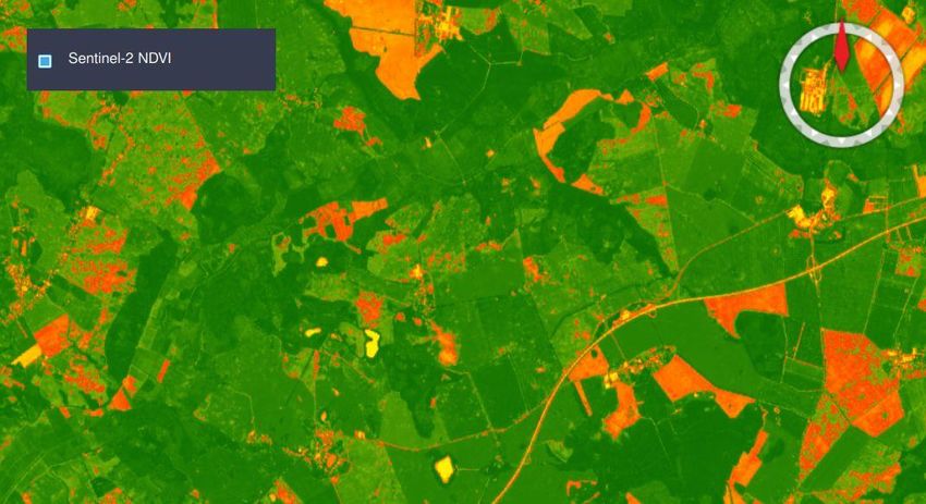
The BigDataToolbox has a WMS example based on NASA WebWorldWind. From original Sentinel-2
data, it shows an NDVI layer which is calculated on the fly with a WCPS query fragment style. This is a
unique capability of the BigDataToolbox WMS server, which allows to build flexible map visualization
without needing to persist pre-calculated layers (and thereby waste expensive disk storage on the
server).
Figure 7 WMS demo screenshot
Page 29 of 43D3.11 Big Data Toolbox Training Manual II
6. Clients
6.1 Rasdaman WSClient
WSClient is a web-client application to interact with WCS (version 2.0.1) and WMS (version 1.3.0)
compliant servers. Once rasdaman is installed it is usually accessible at
http://localhost:8080/rasdaman/ows; a publicly accessible example is available at
https://mundi.rasdaman.com/rasdaman/ows and https://ows.rasdaman.org/rasdaman/ows. The
client has three main tabs: OGC Web Coverage Service (WCS), OGC Web Map Service
(WMS) and Admin. Further on, the functionality in each tab is described in details.
6.1.1 WCS
There are sub-tabs for each of OGC WCS standard requests: GetCapabilities, DescribeCoverage,
GetCoverage, ProcessCoverages.
GetCapabilities
This is the default tab when accessing the WSClient. It lists all coverages available at the specified
WCS endpoint. Clicking on the Get Capabilities button will reload the coverages list. One can
also search a coverage by typing the first characters of its name in the text box. Clicking on a coverage
name will move to DescribeCoverage tab to view its metadata.
Figure 8 List of coverages shown on the GetCapabilities tab.
Page 30 of 43D3.11 Big Data Toolbox Training Manual II
If a coverage is geo-referenced, a checkbox will be visible in the Display footprints column,
allowing to view the coverage’s geo bounding box (in EPSG:4326) on the globe below.
Figure 9 Selected coverage footprints shown on a globe.
At the bottom the metadata of the OGC WCS service endpoint are shown. These metadata can be
changed in the Admin -> OWS Metadata Management tab. Once updated in the admin tab, click
on Get Capabilities button to see the new metadata.
Figure 10 WCS service metadata.
DescribeCoverage
Page 31 of 43D3.11 Big Data Toolbox Training Manual II
Here the full description of a selected coverage can be seen. One can type the first few characters to
search for a coverage id and click on Describe Coverage button to view its OGC WCS metadata.
Figure 11 Showing full description of a coverage.
Once logged in as admin, it’s possible to replace the metadata with one from a valid XML or JSON file.
Figure 12 Updating the metadata of a coverage.
GetCoverage
Downloading coverage data can be done on this tab (or the next one, ProcessCoverages). It’s
similiarly possible search for a coverage id in the text box and click on Select Coverage button to
view its boundaries. Depending on the coverage dimension, one can do trim or slice subsets on the
corresponding axes to select an area of interest. The output format can be selected (provided it
supports the output dimension). Finally, clicking on Get Coverage button will download the
coverage.
Page 32 of 43D3.11 Big Data Toolbox Training Manual II
Figure 13 Downloading a subset of a coverage, encoded in image/tiff.
In addition, further parameters can be specified as supported by the WCS extensions, e.g. scaling
factor, output CRS, subset of ranges (bands), etc.
ProcessCoverages
WCPS queries can be typed in a text box. Once Excute is clicked, the result will be
• displayed on the output console if it’s a scalar or the query was prefixed with image>> (for
2D png/jpeg) or diagram>> for (1D csv/json);
• otherwise it will be downloaded.
Page 33 of 43D3.11 Big Data Toolbox Training Manual II
Figure 14 Query and output areas on the ProcessCoverages tab.
DeleteCoverage
This tab allows to delete a specific coverage from the server. It is only visible when logged in the
Admin tab.
Figure 15 Deleting coverage test_DaysPerMonth.
InsertCoverage
Similarly, this tab is only visible when logged in the Admin tab. To insert a coverage, a URL pointing to
a valid coverage definition according to the WCS-T standard needs to be provided. Clicking on Insert
Coverage button will invoke the correct WCS-T request on the server.
Figure 16 Inserting a coverage given a URL pointing to a valid GML document.
Page 34 of 43D3.11 Big Data Toolbox Training Manual II
6.1.2 WMS
This tab contain sub-tabs which are related to the supported OGC WMS requests.
GetCapabilities
This tab lists the available layers on the specified server. To reload the list, click on the Get
Capabilities button. Clicking on a layer name will move to DescribeLayer tab to view its
description.
Figure 17 List of layers shown on the GetCapabilities tab.
Similar to the WCS GetCapabilities tab, it’s possible to search for layer names, or show their
footprints.
Page 35 of 43D3.11 Big Data Toolbox Training Manual II
Figure 18 Selected layer footprints shown on a globe.
DescribeLayer
Here the full description of a selected layer is shown. One can type the first few characters to search
for a layer name and click on Describe Layer button to view its OGC WMS metadata.
Figure 19 Showing full description of a layer.
Depending on layer’s dimension, one can click on show layer button and interact with axes’ sliders to
view a layer’s slice on the globe below. Click on the hide layer button to hide the displayed layer on
the globe.
Page 36 of 43D3.11 Big Data Toolbox Training Manual II
Figure 20 Showing/hiding a layer on the map.
Finally, managing WMS styles is possible on this tab. To create a style, it is required to input various
parameters along with a rasql or WCPS query fragment, which are applied on every GetMap request
if the style is active. Afterwards, click on Insert Style to insert a new style or Update Style to update
an existing style of the current selected layer. One can also delete an existing style by clicking on the
Delete button corresponding to a style name.
Page 37 of 43You can also read