R-GAP: RECURSIVE GRADIENT ATTACK ON PRIVACY
←
→
Page content transcription
If your browser does not render page correctly, please read the page content below
Published as a conference paper at ICLR 2021

R-GAP: R ECURSIVE G RADIENT ATTACK ON P RIVACY

                                  Junyi Zhu and Matthew Blaschko

                     Dept. ESAT, Center for Processing Speech and Images
                                   KU Leuven, Belgium
                 {junyi.zhu,matthew.blaschko}@esat.kuleuven.be

                                             A BSTRACT

         Federated learning frameworks have been regarded as a promising approach to
         break the dilemma between demands on privacy and the promise of learning from
         large collections of distributed data. Many such frameworks only ask collaborators
         to share their local update of a common model, i.e. gradients, instead of exposing
         their raw data to other collaborators. However, recent optimization-based gradi-
         ent attacks show that raw data can often be accurately recovered from gradients. It
         has been shown that minimizing the Euclidean distance between true gradients and
         those calculated from estimated data is often effective in fully recovering private
         data. However, there is a fundamental lack of theoretical understanding of how
         and when gradients can lead to unique recovery of original data. Our research fills
         this gap by providing a closed-form recursive procedure to recover data from gra-
         dients in deep neural networks. We name it Recursive Gradient Attack on Privacy
         (R-GAP). Experimental results demonstrate that R-GAP works as well as or even
         better than optimization-based approaches at a fraction of the computation under
         certain conditions. Additionally, we propose a Rank Analysis method, which can
         be used to estimate the risk of gradient attacks inherent in certain network ar-
         chitectures, regardless of whether an optimization-based or closed-form-recursive
         attack is used. Experimental results demonstrate the utility of the rank analysis
         towards improving the network’s security. Source code is available for download
         from https://github.com/JunyiZhu-AI/R-GAP.

1   I NTRODUCTION

Distributed and federated learning have become common strategies for training neural networks
without transferring data (Jochems et al., 2016; 2017; Konečný et al., 2016; McMahan et al., 2017).
Instead, model updates, often in the form of gradients, are exchanged between participating nodes.
These are then used to update at each node a copy of the model. This has been widely applied for
privacy purposes (Rigaki & Garcia, 2020; Cristofaro, 2020), including with medical data (Jochems
et al., 2016; 2017). Recently, it has been demonstrated that this family of approaches is susceptible
to attacks that can in some circumstances recover the training data from the gradient information
exchanged in such federated learning approaches, calling into question their suitability for privacy
preserving distributed machine learning (Phong et al., 2018; Wang et al., 2019; Zhu et al., 2019;
Zhao et al., 2020; Geiping et al., 2020; Wei et al., 2020). To date these attack strategies have
broadly fallen into two groups: (i) an analytical attack based on the use of gradients with respect to
a bias term (Phong et al., 2018), and (ii) an optimization-based attack (Zhu et al., 2019) that can in
some circumstances recover individual training samples in a batch, but that involves a difficult non-
convex optimization that doesn’t always converge to a correct solution (Geiping et al., 2020), and
that provides comparatively little insights into the information that is being exploited in the attack.
The development of privacy attacks is most important because they inform strategies for protecting
against them. This is achieved by perturbations to the transferred gradients, and the form of the
attack can give insights into the type of perturbation that can effectively protect the data (Fan et al.,
2020). As such, the development of novel closed-form attacks is essential to the analysis of privacy
in federated learning. More broadly, the existence of model inversion attacks (He et al., 2019;
Wang et al., 2019; Yang et al., 2019; Zhang et al., 2020) calls into question whether transferring

                                                   1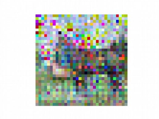
Published as a conference paper at ICLR 2021

a fully trained model can be considered privacy preserving. As the weights of a model trained
by (stochastic) gradient descent are the summation of individual gradients, understanding gradient
attacks can assist in the analysis of and protection against model inversion attacks in and outside of
a federated learning setting.
In this work, we develop a novel third family of attacks, recursive gradient attack on privacy (R-
GAP), that is based on a recursive, depth-wise algorithm for recovering training data from gradient
information. Different from the analytical attack using the bias term, R-GAP utilizes much more
information and is the first closed-form algorithm that works on both convolutional networks and
fully connected networks with or without bias term. Compared to optimization-based attacks, it
is not susceptible to local optima, and is orders of magnitude faster to run with a deterministic
running time. Furthermore, we show that under certain conditions our recursive attack can fully
recover training data in cases where optimization attacks fail. Additionally, the insights gained from
the closed form of our recursive attack have lead to a refined rank analysis that predicts which
network architectures enable full recovery, and which lead to provable noisy recovery due to rank-
deficiency. This explains well the performance of both closed-form and optimization-based attacks.
We also demonstrate that using rank analysis we are able to make small modifications to network
architectures to increase the network’s security without sacrificing its accuracy.

1.1   R ELATED W ORK

Bias attacks: The original discovery of the existence of an analytical attack based on gradients with
respect to the bias term is due to Phong et al. (2018). Fan et al. (2020) also analyzed the bias attack
as a system of linear equations, and proposed a method of perturbing the gradients to protect against
it. Their work considers convolutional and fully-connected networks as equivalent, but this ignores
the aggregation of gradients in convolutional networks. Similar to our work, they also perform a
rank analysis, but it considers fewer constraints than is included in our analysis (Section 4).
Optimization attacks: The first attack that utilized an optimization approach to minimize the dis-
tance between gradients appears to be due to Wang et al. (2019). In this work, optimization is
adopted as a submodule in their GAN-style framework. Subsequently, Zhu et al. (2019) proposed
a method called deep leakage from gradients (DLG) which relies entirely on minimization of the
difference of gradients (Section 2). They propose the use of L-BFGS (Liu & Nocedal, 1989) to
perform the optimization. Zhao et al. (2020) further analyzed label inference in this setting, propos-
ing an analytic way to reconstruct the one-hot label of multi-class classification in terms of a single
input. Wei et al. (2020) show that DLG is sensitive to initialization and proposed that the same
class image is an optimal initialization. They proposed to use SSIM as image similarity metric,
which can then be used to guide optimization by DLG. Geiping et al. (2020) point out that as DLG
requires second-order derivatives, L-BFGS actually requires third-order derivatives, which leads
to challenging optimzation for networks with activation functions such as ReLU and LeakyReLU.
They therefore propose to replace L-BFGS with Adam (Kingma & Ba, 2015). Similar to the work
of Wei et al. (2020), Geiping et al. (2020) propose to incorporate an image prior, in this case total
variation, while using PSNR as a quality measurement.

2     O PTIMIZATION -BASED G RADIENT ATTACKS ON P RIVACY (O-GAP)
Optimization-based gradient attacks on privacy (O-GAP) take the real gradients as its ground-truth
label and utilizes optimization to decrease the distance between the real gradients ∇W and the
dummy gradients ∇W0 generated by a pair of randomly initialized dummy data and dummy label.
The objective function of O-GAP can be generally expressed as:
                                                         d
                                                         X
                                         0 2
                    arg min
                         0 0
                             k∇W   − ∇W   k  =  arg min
                                                     0 0
                                                            k∇Wi − ∇W0i k2 ,                   (1)
                        x ,y                          x ,y
                                                             i=1
where the summation is taken over the layers of a network of depth d, and (x0 , y 0 ) is the dummy
training data and label used to generate ∇W 0 . The idea of O-GAP was proposed by Wang et al.
(2019). However, they have adopted it as a part of their GAN-style framework and did not realize
that O-GAP is able to preform a more accurate attack by itself. Later in the work of Zhu et al.
(2019), O-GAP has been proposed as a stand alone approach, the framework has been named as
Deep Leakage from Gradients (DLG).

                                                  2
Published as a conference paper at ICLR 2021
The approach is intuitively simple, and in practice has been shown to give surprisingly good re-
sults (Zhu et al., 2019). However, it is sensitive to initialization and prone to fail (Zhao et al.,
2020). The choice of optimizer is therefore important, and convergence can be very slow (Geip-
ing et al., 2020). Perhaps most importantly, Equation 1 gives little insight into what information
in the gradients is being exploited to recover the data. Analysis in Zhu et al. (2019) is limited
to empirical insights, and fundamental open questions remain: What are sufficient conditions for
Pd
arg minx0 ,y0 i=1 k∇Wi − ∇W0i k2 to have a unique minimizer? We address this question in Sec-
tion 4, and subsequently validate our findings empirically.
3 C LOSED -F ORM G RADIENT ATTACKS ON P RIVACY
The first attempt of closed-form GAP was proposed in a research of privacy-preserving deep learning
by Phong et al. (2018).
Theorem 1 (Phong et al. (2018)). Assume a layer of a fully connected network with a bias term,
expressed as:
Wx + b = z, (2)
where W, b denote the weight matrix and bias vector, and x, z denote the input vector and output
vector of this layer. If the loss function ` of the network can be expressed as:
` = `(f (x), y)
where f indicates a nested function of x including activation function and all subsequent layers, y
is the ground-truth label. Then x can be derived from gradients w.r.t. W and gradients w.r.t. b, i.e.:
∂` ∂` > ∂` ∂`
= x , =
∂W ∂z ∂b ∂z
∂` ∂`
x> = / (3)
∂Wj ∂bj
where j denotes the j-th row, note that in fact from each row we can compute a copy of x> .
When this layer is the first layer of a network, it is possible to reconstruct the data, i.e. x, using this
approach. In the case of noisy gradients, we can make use of the redundancy in estimating x by
averaging over noisy estimates: x̂> = j ∂W
P ∂` ∂`
j
/ ∂bj . However, simply removing the bias term can
disable this attack. Besides, this approach does not work on convolutional neural networks due to a
dimension mismatch in Equation 3. Both of these two problems have been resolved in our approach.
3.1 R ECURSIVE GRADIENT ATTACK ON PRIVACY (R-GAP)
For simplicity we derive the R-GAP in terms of binary classification with a single image as input.
In this setting we can generally describe the network and loss function as:
=:fd−1 (x)
z }| {
µ = ywd σd−1 Wd−1 σd−2 (Wd−2 φ (x)) (4)
| {z }
=:fd−2 (x)
−µ
` = log(1 + e ) (5)
where y ∈ {−1, 1}, d denotes the d-th layer, φ represents all layers previous to d − 2, and σ denotes
the activation function. Note that, although our notation omits the bias term in our approach, with
an augmented matrix and augmented vector it is able to represent both of the linear map and the
translation, e.g. Equation 2, using matrix multiplication as shown in Equation 4. So our formulation
also includes the approach proposed by Phong et al. (2018). Moreover, if the i-th layer is a convo-
lutional layer, then Wi is an extended circulant matrix representing the convolutional kernel (Golub
& Van Loan, 1996), and data x as well as input of each layer are represented by a flattened vector in
Equation 4.
3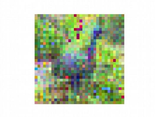
Published as a conference paper at ICLR 2021

               ∂`                                    ∂`                                        ∂`
               ∂µ
                  µ                                  ∂µ
                                                        µ                                      ∂µ
                                                                                                  µ

                               µ                                     µ                                     µ

           `: Logistic loss                    `: Exponential loss                    `: Hinge loss

                                                                                   ∂`
Figure 1: In consideration of logistic loss, exponential loss and hinge loss, ∂µ      µ is not monotonic
                                                                        −
w.r.t. µ. It is equal to 0 at µ = 0, after that it either approximates 0 , or equals to 0 after decreasing
to µ = 1.

3.1.1    R ECOVERING DATA FROM GRADIENTS
From Equation 4 and Equation 5 we can derive following gradients:
                        ∂`         ∂` >
                               = y fd−1                                                                      (6)
                       ∂wd         ∂µ

                      ∂`                    ∂`
                               =     w>
                                      d   y             σ 0
                                                          d−1 fd−2
                                                                   >
                                                                                                             (7)
                   ∂Wd−1                    ∂µ

                      ∂`                                ∂`
                               =     W>d−1     w >
                                                 d    y             σ 0
                                                                      d−1        σ 0
                                                                                  d−2 φ
                                                                                           >
                                                                                                             (8)
                   ∂Wd−2                                ∂µ
where σ 0 denotes the derivative of σ, for more details of deriving the gradients refer to Appendix H.
The first observation of these gradients is that:
                                              ∂`              ∂`
                                                   · wd =        µ                                           (9)
                                             ∂wd             ∂µ
Additionally, if σ1 , ... , σd−1 are ReLU or LeakyRelu, the dot product of the gradients and weights
of each layer will be the same, i.e.:
                         ∂`              ∂`                          ∂`              ∂`
                               · wd =          · Wd−1 = ... =             · W1 =        µ                  (10)
                       ∂wd            ∂Wd−1                         ∂W1             ∂µ
                                                                            ∂`
Since gradients and weights of each layer are known, we can obtain ∂µ          µ. If loss function ` is logistic
loss (Equation 5), we obtain:
                                              ∂`            −µ
                                                  µ=             .                                         (11)
                                              ∂µ        1 + eµ
                                                              ∂`                       ∂`
In order to perform R-GAP, we need to derive µ from ∂µ           µ. As we can see, ∂µ     µ is non-monotonic,
                            ∂`
which means knowing ∂µ µ does not always allow us to uniquely recover µ. However, even in the
case that we cannot uniquely recover µ, there are only two possible values to consider. Figure 1
            ∂`
illustrates ∂µ µ of logistic, exponential, and hinge losses, showing when we can uniquely recover µ
       ∂`
from ∂µ µ. The non-uniqueness of µ inspires us to find a sort of data that can trigger exactly the
same gradients as the real data, which we name twin data, denoted by x̃. The existence of twin data
demonstrates that the objective function of DLG could have more than one global minimum, which
explains at least in part why DLG is sensitive to initialization, for more information and experiments
about the twin data refer to Appendix B.
The second observation on Equations 6-8 is that the gradients of each layer have a repeated format:
                          ∂`         >              ∂`
                              = kd fd−1  ; kd := y                                             (12)
                         ∂wd                        ∂µ
                         ∂`            >
                                            ; kd−1 := w>             0

                              = kd−1 fd−2                 d kd      σd−1                       (13)
                      ∂Wd−1
                         ∂`
                              = kd−2 φ> ; kd−2 := W>                     0

                                                         d−1 kd−1      σd−2                    (14)
                      ∂Wd−2

                                                       4
Published as a conference paper at ICLR 2021

In Equation 12, the value of y can be derived from the sign of the gradients at this layer if the acti-
vation function of previous layer is ReLU or Sigmoid, i.e. fd−1 > 0. For multi-class classification,
y can always be analytically derived as proved by Zhao et al. (2020). From Equations 12-14 we can
see that gradients are actually linear constraints on the output of the previous layer, also the input of
the current layer. We name these gradient constraints, which can be generally described as:
                                                            ∂`
                                        Ki xi = flatten(       ),                                   (15)
                                                           ∂Wi
where i denotes i-th layer, xi denotes the input and Ki is a coefficient matrix containing all gradient
constraints at the i-th layer.

3.1.2   I MPLEMENTATION OF R-GAP
                                                 ∂`
To reconstruct the input xi from the gradients ∂W   i
                                                      at the i-th layer, we need to determine Ki or ki .
The coefficient vector ki solely relies on the reconstruction of the subsequent layer. For example
                                             0                                         0
in Equation 13, kd−1 consists of wd , kd , σd−1 , where wd is known, and kd and σd−1       are products
of the reconstruction at the d-th layer. More specifically, kd can be calculated by deriving y and
                                    0
µ as described in Section 3.1.1, σd−1   can be derived from the reconstructed fd−1 . The condition
for recovering xi under gradient constraints ki is that the rank of the coefficient matrix equals the
number of entries of the input, rank(Ki ) = |xi |. Furthermore, if this rank condition holds for
i = 1, ..., d, we are able to reconstruct the input at each layer and do this recursively back to the
input of the first layer.
The number of gradient constraints is the same as the number of weights, i.e. rows(Ki ) = |Wi |; i =
1, ..., d. Specifically, in the case of a fully connected layer we always have rank(Ki ) = |xi |, which
implies the reconstruction over FCNs is always feasible. However in the case of a convolutional
layer the matrix could possibly be rank-deficient to derive x. Fortunately, from the view of recursive
reconstruction and assuming we know the input of the subsequent layer, i.e. the output of the current
layer, there is a new group of linear constraints which we name weight constraints:
                                        Wi xi = zi ;   zi ← fi                                      (16)
For a convolution layer, the Wi we use in this paper is the corresponding circulant matrix represent-
ing the convolutional kernel (Golub & Van Loan, 1996), so we can express the convolution in the
form of Equation 16. In order to derive zi from fi , the activation function σi should be monotonic.
Commonly used activation functions satisfy this requirement. Note that for the ReLU activation
function, a 0 value in fi will remove a constraint in Wi . Otherwise, the number of weights con-
straints is equal to the number of entries in output, i.e. rows(Wi ) = |zi |; i = 1, ..., d. In CNNs
the number of weight constraints |zi | is much larger than the number of gradient constraints |Wi | in
bottom layers, and well compensate for the lack of gradient constraints in those layers. It is worth
noting that, due to the transformation from a CNN to a FCN using the circulant matrix, a CNN has
been regarded equivalent to a FCN in the parallel work of Fan et al. (2020). However, we would like
to point out that in consideration of the gradients w.r.t. the circulant matrix, what we obtain from
a CNN are the aggregated gradients. Therefore, the number of valid gradient constraints in a CNN
are much smaller than its corresponding FCN. Therefore, the conclusion of a rank analysis derived
from a FCN cannot be directly applied to a CNN.
Moreover, padding in the i-th convolutional layer increases |xi |, but also involves the same number
of constraints, so we omit this detail in the subsequent discussion. However, we have incorporated
the corresponding constraints in our approach. Based on gradient constraints and weight constraints,
we break the gradient attacks down to a recursive process of solving systems of linear equations,
which we name R-GAP . The approach is detailed in Algorithm 1.

4   R ANK ANALYSIS
For optimization-based gradient attacks such as DLG, it is hard to estimate whether it will converge
to a unique solution given a network’s architecture other than performing an empirical test. An
intuitive assumption would be that the more parameters in the model, the greater the chance of
unique recovery, since there will be more terms in the objective function constraining the solution.
We provide here an analytic approach, with which it is easy to estimate the feasibility of performing

                                                   5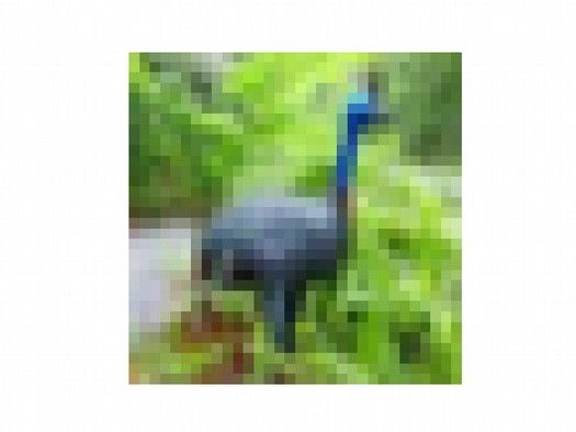
Published as a conference paper at ICLR 2021

Algorithm 1: R-GAP (Notation is consistent with Equation 6 to Equation 15)
Data: i: i-th layer; Wi : weights; ∇Wi : gradients;
Result: x1
for i ← d to 1 do
    if i = d then
          ∂`
         ∂µ µ = ∇Wi · Wi ;
         µ ← ∂µ  ∂`            ∂`
                    µ; ki := y ∂µ ; zi := µy ;
    else
         /* Derive σi0 and zi from fi . Note that xi+1 = fi .                                       */
         σi0 ← xi+1 ; zi ← xi+1 ;
         ki := (W>   i+1 ki+1 )    σi0 ;
    end
    Ki ←    ki ; ∇w
                    i := flatten(∇W
                                    i );
              Wi               zi
    Ai :=           ; bi :=           ;
              Ki             ∇w i
    xi := A†i bi // A†i :Moore-Penrose pseudoinverse
end

the recursive gradient attack, which in turn is a good proxy to estimate when DLG converges to a
good solution (see Figure 2).
Since R-GAP solves a sequence of linear equations, it is infeasible when the number of unknown
parameters is more than the number of constraints at any i-th layer, i.e. |xi | − |Wi | − |zi | > 0. More
precisely, R-GAP requires that the rank of Ai , which consists of Wi and Ki as shown in Algorithm 1,
is equal to the number of input entries |xi |. However, Ai xi = zi does not include all effective
constraints over xi . Because xi is unique to zi−1 or partly unique in terms of the ReLU activation
function, any constraint over zi−1 will limit the possible value of xi . On that note, suppose |xi−1 | =
m, |zi−1 | = n and the weight constraints at the i − 1 layer is overdetermined, i.e. Wi−1 xi−1 =
zi−1 ; m < n, rank(Wi−1 ) = m. Without the loss of generality, let the first m entries of zi−1 be
linearly independent, the m + 1, . . . , n entries of zi−1 can be expressed as linear combination of the
first m entries, i.e. Mz1,
                        i−1
                           ..., m
                                  = zm+1,
                                     i−1
                                          ..., n
                                                 . In other words, if the previous layers are overdetermined
by weight constraints, the subsequent layer will have additional constraints, not merely its local
weight constraints and gradient constraints. Since this type of additional constraint is not derived
from the parameters of the layer that under reconstruction, we name them virtual constraints denoted
by V. When the activation function is the identity function, the virtual constraints are linear and can
be readily derived. For the derivative of the activation function not being a constant, the virtual
constraints will become non-linear. For more details about deriving the virtual constraints, refer to
Appendix C. Optimization based attacks such as DLG are iterative algorithms based on gradient
descent, and are able to implicitly utilize the non-linear virtual constraints. Therefore to provide
a comprehensive estimate of the data vulnerability under gradient attacks, we also have to count
the number of virtual constraints. It is worth noticing that virtual constraints can be passed along
through the linear equation systems chain, but only in one direction that is to the subsequent layers.
Next, we will informally use |Vi | to denote the number of virtual constraints at the i-th layer, which
                           Pi−1
can be approximated by n=1 max(|zn | − |xn |, 0) − max(|xn | − |zn | − |Wn |, 0). For more details
refer to Appendix C. In practice, the real number of such constraints is dependent on the data, current
weights, and choice of activation function.
These three types of constraints, gradient, weight and virtual constraints, are effective for predicting
the risk of gradient attack. To conclude, we propose that |xi | − |Wi | − |zi | − |Vi | is a good index
to estimate the feasibility of fully recovering the input using gradient attacks at the i-th layer. We
denote this value rank analysis index (RA-i). Particularly, |xi | − |Wi | − |zi | − |Vi | > 0 indicates
it is not possible to perform a complete reconstruction of the input, and the larger this index is, the
poorer the quality of reconstruction will be. If the constraints in a particular problem are linearly
independent, |xi | − |Wi | − |zi | − |Vi | < 0 implies the ability to fully recover the input. The quality
of reconstruction of data is well estimated by the maximal RA-i of all layers, as shown in Figure 2.
In practice, the layers close to the data usually have smaller RA-i due to fewer virtual constraints.

                                                     6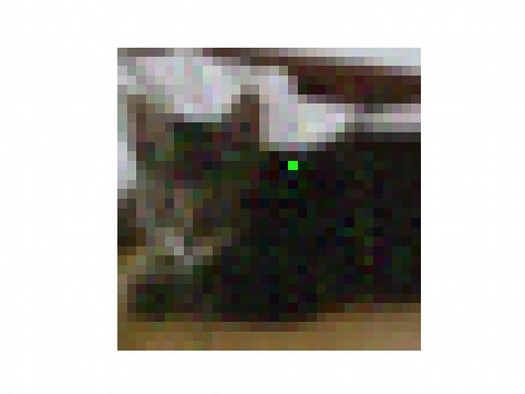
Published as a conference paper at ICLR 2021
Image Image Image Image Image
Architecture conv1 4x4@4 conv1 4x4@3 conv1 4x4@3 conv1 3x3@4 conv1 5x5@4
3364x1 fc 2523x1 fc 2523x500 fc conv2 3x3@4 conv2 4x4@4
500x1 fc 3136x1 fc 2500x1 fc
|W| = 3556 |W| = 2667 |W| = 1.26x10⁶ |W| = 3388 |W| = 3056
conv1: conv1: conv1: conv1: conv1:
Rank |x1| - |W1| - |z1| < 0 |x1| - |W1| - |z1| > 0 |x1| - |W1| - |z1| > 0 |x1| - |W1| - |z1| < 0 |x1| - |W1| - |z1| < 0
Analysis conv2: conv2:
|x2| - |W2| - |z2| > 0 |x2| - |W2| - |z2| > 0
|x2| - |W2| - |z2| - |V2| < 0 |x2| - |W2| - |z2| - |V2| > 0
DLG
Reconstruction
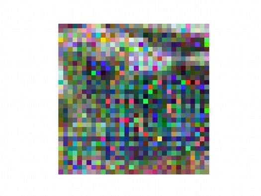
Figure 2: Estimating the privacy leakage of network through rank analysis. The critical layer for
reconstruction has been red colored. First three columns show that even though bigger network has
much more parameters denoted by |W|, which means we can collect more gradients to reconstruct
the data, but if the layer close to data is rank-deficient, we are not able to fully recover the data.
Despite that in the objective function of DLG, distance between all gradients will be reduced at
the same time, redundant constraints in subsequent layer certainly cannot compensate the lack of
constraints in previous layer. The fourth column shows that if rank-deficiency happens at the in-
termediate layer, redundant weight constraints in previous layer, i.e. virtual constraints, is able to
compensate the deficiency at the intermediate layer. If a layer is rank-deficient after taking virtual
constraints into account, fully recovery is again not possible as shown in the fifth column. However,
as the rank analysis index of last column is smaller than the one of the second and third column, the
reconstruction at the fifth column has a better quality. This figure demonstrates that rank analysis
can correctly estimate the feasibility of performing DLG, for statistic result refer to Appendix A.
On top of that we analyse the residual block in ResNet, which shows some interesting traits of the
skip connection in terms of the rank-deficiency, for more details refer to Appendix D.
A valuable observation we obtain through the rank analysis is that the architecture rather than the
number of parameters is critical to gradient attacks, as shown in Figure 2. This observation is
not obvious from simply specifying the DLG optimization problem(see Equation 1). Furthermore,
since the data vulnerability of a network depends on the layer with maximal RA-i, we can design
rank-deficiency into the architecture to improve the security of a network (see Figure 4).
5 R ESULTS
Our novel approach R-GAP successfully extends the analytic gradient attack (Phong et al., 2018)
from attacking a FCN with bias terms to attacking FCNs and CNNs1 with or without bias terms. To
test its performance, we use a CNN6 network as shown in Figure 3, which is full-rank considering
gradient constraints and weight constraints. Additionally, we report results using a CNN6-d network,
which is rank-deficient without consideration of virtual constraints, in order to to fairly compare the
performance of DLG and R-GAP. CNN6-d has a CNN6 backbone and just decreases the output
channel of the second convolutional layer to 20. The activation function is a LeakyReLU except
the last layer, which is a Sigmoid. We have randomly initialized the network, as DLG is prone to
fail if the network is at a late stage of training (Geiping et al., 2020). Furthermore, as the label
can be analytically recovered by R-GAP, we always provide DLG the ground-truth label and let it
recover the image only. Therefore the experiment actually compares R-GAP with iDLG (Zhao et al.,
2020). The experimental results show that, due to an analytic one-shot process, run-time of R-GAP
is orders of magnitude shorter than DLG. Moreover, R-GAP can recover the data more accurately,
1
via equivalence between convolution and multiplication with a (block) circulant matrix.
7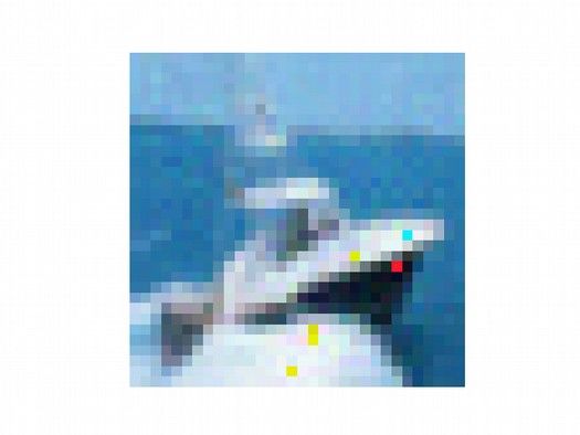
Published as a conference paper at ICLR 2021

while optimization-based methods like DLG recover the data with artifacts, as shown in Figure 3.
The statistical results in Table 1 also show that the reconstruction of R-GAP has a much lower
MSE than DLG on the CNN6 network. However, as R-GAP only considers gradient constraints and
weight constraints in the current implementation, it does not work well on the CNN6-d network.
Nonetheless, we find that it is easy to assess the quality of reconstruction of gradient attack without
knowing the original image. As the better reconstruction has less salt-and-pepper type noise. We
measure this by the difference of the image and its smoothed version (achieved by a simple 3x3
averaging) and select the output with the smaller norm. This hybrid approach which we name H-
GAP combines the strengths of R-GAP and DLG, and obtains the best results.

                      Architecture                 Origin
                         Image
                     conv1 4x4@12, /2
                     conv2 3x3@36, /2
                                                   Our
                        conv3 3x3@36             approach
                        conv4 3x3@36
                     conv5 3x3@64, /2
                       conv6 3x3@128
                         3200x1 fc                  DLG

Figure 3: Performance of our approach and DLG over a CNN6 architecture. The diagram on the
left demonstrates the network architecture on which we perform attack. The activation functions are
LeakyReLU, except the last one which is Sigmoid.

                     CNN6*             CNN6-d*              CNN6**                                       CNN6-d**
   R-GAP         0.010 ± 0.0017       1.4 ± 0.073   1.9 × 10⁻⁴ ± 7.0 × 10⁻⁵                         0.0090 ± 9.3 × 10⁻⁴
    DLG          0.050 ± 0.0014     0.053 ± 0.0016  4.2 × 10⁻⁴ ± 5.9 × 10⁻⁵                        0.0012 ± 1.8 × 10⁻⁴
   H-GAP        0.0069 ± 0.0012     0.053 ± 0.0016 1.4 × 10⁻⁴ ± 2.3 × 10⁻⁵                         0.0012 ± 1.8 × 10⁻⁴
                                *:CIFAR10 **:MNIST

Table 1: Comparison of the performance of R-GAP, DLG and H-GAP. MSE has been used to mea-
sure the quality of the reconstruction.

Moreover, we compare R-GAP with DLG on LeNet which has been benchmarked in DLG(Zhu
et al., 2019), the statistical results are shown in Table 2. Both DLG and R-GAP perform well on
LeNet. Empirically, if the MSE is around or below 1×10⁻⁴ , the difference of the reconstruction will
be visually undetectable. However, we surprisingly find that by replacing the Sigmoid function with
the Leaky ReLU, the reconstruction of DLG becomes much poorer. The condition number of matrix
A (from Algorithm 1) changes significantly in this case. Since the Sigmoid function leads to a higher
condition number at each convolutional layer, reconstruction error in the subsequent layer could be
amplified in the previous layer, therefore DLG is forced to converge to a better result. In contrast,
R-GAP has an accumulated error and naturally performs much better on LeNet*. Additionally, we
find R-GAP could be a good initialization tool for DLG. As shown in the last column of Table 2,
by initializing DLG with the reconstruction of R-GAP, and running 8% of the previous iterations,
we achieve a visually indistinguishable result. However, for LeNet*, we find that DLG reduces the
reconstruction quality obtained by R-GAP, which further shows the instability of DLG.
Our rank analysis is a useful offline tool to understand the risk inherent in certain network architec-
tures. More precisely, we can use the rank analysis to find out the critical layer for the success of

                               Condition number                                                MSE
                    conv1          conv2             conv3               DLG                  R-GAP           R-GAP→ DLG
                                                                                −8
       LeNet      1.8 × 10⁴
                                 6.1 × 10   3
                                                      32.4           3.7 × 10              1.1 × 10⁻⁴          1.1 × 10⁻⁶
                    ±2.9           ±0.3         ±2.9 × 10⁻⁴         ±8.6 × 10⁻¹⁰         ±7.8 × 10⁻⁶          ±1.1 × 10⁻⁶
       LeNet*     1.2 × 10³      1.3 × 10³            14.2           5.2 × 10⁻²           1.5 × 10⁻¹⁰          4.8 × 10⁻⁴
                    ±19.7          ±22.5             ±0.05          ±2.9 × 10⁻³          ±2.5 × 10⁻¹¹         ±9.1 × 10⁻⁵
                      LeNet* is identical to LeNet but uses Leaky ReLU activation function instead of Sigmoid

   Table 2: Comparison of R-GAP and DLG on LeNet benchmarked in DLG(Zhu et al., 2019).

                                                               8
Published as a conference paper at ICLR 2021

gradient attacks and take precision measurements to improve the network’s defendability. We report
results on the ResNet-18, where the third residual block is critical since by cutting its skip connec-
tion the RA-i increases substantially. To perform the experiments, we use the approach proposed
by Geiping et al. (2020), which extends DLG to incorporate image priors and performs better on
deep networks. As shown in Figure 4, by cutting the skip connection of the third residual block,
reconstructions become significantly poorer and more unstable. As a control test, cutting the skip
connection of a non-critical residual block does not increase defendability noticeably. Note that two
variants have the same or even slightly better performance on the classification task compared with
the backbone. In previous works (Zhu et al., 2019; Wei et al., 2020), trade-off between accuracy and
defendability of adding noise to gradients has been discussed. We show that using the rank analysis
we are able to increase the defendability of a network with no cost in accuracy.

        Image

      conv 3x3@16
                                   Origin

     residual block 1
         3x3@16                  ResNet18

     residual block 2
         3x3@16                  Variant 1

     residual block 3
       3x3@32, /2       1        Variant 2

     residual block 8
        3x3@128         2
      avgpool 4x4

      dense 128x10

Figure 4: Left: Architectures of the ResNet18 with base width 16 and two variants. Variant 1
cuts the skip connection of the third residual block. Variant 2 cuts the skip connection of the eighth
residual block. Upper right: Reconstruction examples of three networks. Lower right: Accuracy and
reconstruction error of three networks. Training 200 epochs on CIFAR10 and saving the model with
the best performance on the validation set, three networks achieve a close accuracy. Two variants
perform even slightly better. In terms of gradient attacks, MSE of reconstructions from ResNet18
and Variant 2 are similar, since Variant 2 cut the skip connection of a non-critical layer and the
RA-i does not change. Whereas, by cuting the skip connection of a critical layer, according to the
rank analysis, increases RA-i substantially. MSE of the reconstructions from Variant 1 increases by
nearly a factor of three with higher variance.

6   D ISCUSSION AND CONCLUSIONS

R-GAP makes the first step towards a general analytic gradient attack and provides a framework
to answer questions about the functioning of optimization-based attacks. It also opens new ques-
tions, such as how to analytically reconstruct a minibatch of images, especially considering non-
uniqueness due to permutation of the image indices. Nonetheless, we believe that by studying these
questions, we can gain deeper insights into gradient attacks and privacy secure federated learning.
In this paper, we propose a novel approach R-GAP, which has achieved an analytic gradient attack
for CNNs for the first time. Through analysing the recursive reconstruction process, we propose
a novel rank analysis to estimate the feasibility of performing gradient based privacy attacks given
a network architecture. Our rank analysis can be applied to the analysis of both closed-form and
optimization-based attacks such as DLG. Using our rank analysis, we are able to determine network
modifications that maximally improve the network’s security, empirically without sacrificing its
accuracy. Furthermore, we have analyzed the existence of twin data using R-GAP, which can explain
at least in part why DLG is sensitive to initialization and what type of initialization is optimal. In
summary, our work proposes a novel type of gradient attack, a risk estimation tool and advances the
understanding of optimization-based gradient attacks.

                                                  9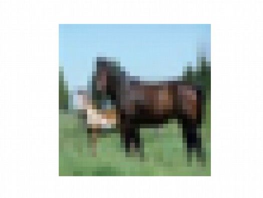
Published as a conference paper at ICLR 2021

ACKNOWLEDGEMENTS

This research received funding from the Flemish Government (AI Research Program).

R EFERENCES
Peter L Bartlett, Michael I Jordan, and Jon D McAuliffe. Convexity, classification, and risk bounds.
  Journal of the American Statistical Association, 101(473):138–156, 2006.
Emiliano De Cristofaro. An overview of privacy in machine learning. arXiv:2005.08679, 2020.
Lixin Fan, Kam Woh Ng, Ce Ju, Tianyu Zhang, Chang Liu, Chee Seng Chan, and Qiang Yang.
  Rethinking privacy preserving deep learning: How to evaluate and thwart privacy attacks. In
  Qiang Yang, Lixin Fan, and Han Yu (eds.), Federated Learning: Privacy and Incentive, pp. 32–
  50. Springer, 2020.
Jonas Geiping, Hartmut Bauermeister, Hannah Dröge, and Michael Moeller. Inverting gradients:
  How easy is it to break privacy in federated learning? In Hugo Larochelle, Marc’Aurelio Ranzato,
  Raia Hadsell, Maria-Florina Balcan, and Hsuan-Tien Lin (eds.), Advances in Neural Information
  Processing Systems 33, 2020.
Gene H. Golub and Charles F. Van Loan. Matrix Computations. Johns Hopkins University Press,
  1996.
Zecheng He, Tianwei Zhang, and Ruby B. Lee. Model inversion attacks against collaborative in-
  ference. In Proceedings of the 35th Annual Computer Security Applications Conference, ACSAC
  ’19, pp. 148–162, 2019.
Arthur Jochems, Timo M. Deist, Johan van Soest, Michael Eble, Paul Bulens, Philippe Coucke,
  Wim Dries, Philippe Lambin, and Andre Dekker. Distributed learning: Developing a predictive
  model based on data from multiple hospitals without data leaving the hospital – a real life proof
  of concept. Radiotherapy and Oncology, 121(3):459 – 467, 2016.
Arthur Jochems, Timo Deist, Issam El Naqa, Marc Kessler, Chuck Mayo, Jackson Reeves, Shruti
  Jolly, Martha Matuszak, Randall Ten Haken, Johan Soest, Cary Oberije, Corinne Faivre-Finn,
  Gareth Price, Dirk Ruysscher, Philippe Lambin, and André Dekker. Developing and validating
  a survival prediction model for nsclc patients through distributed learning across three countries.
  International Journal of Radiation Oncology*Biology*Physics, 99, 04 2017.
Diederik P. Kingma and Jimmy Ba. Adam: A method for stochastic optimization. In Yoshua Bengio
  and Yann LeCun (eds.), 3rd International Conference on Learning Representations, 2015.
Jakub Konečný, H. Brendan McMahan, Felix X. Yu, Peter Richtarik, Ananda Theertha Suresh, and
  Dave Bacon. Federated learning: Strategies for improving communication efficiency. In NIPS
  Workshop on Private Multi-Party Machine Learning, 2016.
Dong C. Liu and Jorge Nocedal. On the limited memory BFGS method for large scale optimization.
  Math. Program., 45(1–3):503–528, August 1989.
Brendan McMahan, Eider Moore, Daniel Ramage, Seth Hampson, and Blaise Aguera y Arcas.
  Communication-efficient learning of deep networks from decentralized data. In Aarti Singh and
  Jerry Zhu (eds.), Proceedings of the 20th International Conference on Artificial Intelligence and
  Statistics, volume 54 of Proceedings of Machine Learning Research, pp. 1273–1282, 2017.
L. T. Phong, Y. Aono, T. Hayashi, L. Wang, and S. Moriai. Privacy-preserving deep learning via
  additively homomorphic encryption. IEEE Transactions on Information Forensics and Security,
  13(5):1333–1345, 2018.
Maria Rigaki and Sebastian Garcia. A survey of privacy attacks in machine learning. CoRR,
 abs/2007.07646, 2020.
Z. Wang, M. Song, Z. Zhang, Y. Song, Q. Wang, and H. Qi. Beyond inferring class representatives:
   User-level privacy leakage from federated learning. In IEEE INFOCOM 2019 - IEEE Conference
   on Computer Communications, pp. 2512–2520, 2019.

                                                 10
Published as a conference paper at ICLR 2021
Wenqi Wei, Ling Liu, Margaret Loper, Ka-Ho Chow, Mehmet Emre Gursoy, Stacey Truex, and
Yanzhao Wu. A framework for evaluating client privacy leakages in federated learning. In Liqun
Chen, Ninghui Li, Kaitai Liang, and Steve Schneider (eds.), Computer Security – ESORICS, pp.
545–566. Springer, 2020.
Ziqi Yang, Jiyi Zhang, Ee-Chien Chang, and Zhenkai Liang. Neural network inversion in adver-
sarial setting via background knowledge alignment. In Proceedings of the 2019 ACM SIGSAC
Conference on Computer and Communications Security, pp. 225–240, 2019.
Yuheng Zhang, Ruoxi Jia, Hengzhi Pei, Wenxiao Wang, Bo Li, and Dawn Song. The secret revealer:
Generative model-inversion attacks against deep neural networks. In IEEE/CVF Conference on
Computer Vision and Pattern Recognition, pp. 250–258, 2020.
Bo Zhao, Konda Reddy Mopuri, and Hakan Bilen. iDLG: Improved deep leakage from gradients.
arXiv:2001.02610, 2020.
Ligeng Zhu, Zhijian Liu, and Song Han. Deep leakage from gradients. In H. Wallach, H. Larochelle,
A. Beygelzimer, F. d’Alché Buc, E. Fox, and R. Garnett (eds.), Advances in Neural Information
Processing Systems 32, pp. 14774–14784, 2019.
A Q UANTITATIVE RESULTS OF RANK ANALYSIS
A quantitative analysis of the predictive performance of the rank analysis index for the mean squared
error of reconstruction is shown in Table 3.
RA-i -484 405 405 -208 316
MSE 4.2 × 10⁻⁹ 0.056 ± 0.0035 0.063 ± 0.004 2.7 × 10⁻⁴ 0.013
±2.2 × 10⁻⁹ ±2.0 × 10⁻⁵ ±7.2 × 10⁻⁴
Table 3: Mean square error of the reconstruction over test set of CIFAR10. The corresponding
network architecture has been shown in Figure 2 in the same order. Rank analysis index (RA-i)
clearly predicts the reconstruction error. We can also regard RA-i as the security level of a network.
A negative value indicates that the gradients of the network are able to fully expose the data, i.e.
insecure, while a positive value indicates that completely recover the data from gradients is not
possible. On top of that, higher RA-i indicate higher reconstruction error, therefore the network is
more secure. According to our experiment, if the order of magnitude of MSE is equal to or less than
10−4 , we could barely visually distinguish the recovered and real data, as shown in the fourth column
of Figure 2. Note that, as the network gets deeper, DLG will become vulnerable, R-GAP will also
be effected by numerical error. Besides that, DLG is sensitive to the initialization of dummy data,
while R-GAP also needs to confirm the µ if it is not unique. Therefore, RA-i provides a reasonable
upper bound of the privacy risk rather than quality prediction of one reconstruction.
B T WIN DATA
∂` ∂`
As we know ∂µ µ is non-monotonic as shown in Figure 1, which means knowing ∂µ µ does not
always allow us to uniquely recover µ. It is relatively straightforward to show that for mono-
∂` ∂`
tonic convex losses (Bartlett et al., 2006), ∂µ µ is invertible for µ < 0, ∂µ µ ≤ 0 for µ ≥ 0,
∂` ∂`
and limµ→∞ ∂µ µ = 0. Due to the non-uniqueness of µ w.r.t to ∂µ µ, we have:
∂` ∂`
∃ x, x̃ s.t. µ 6= µ̃; µ= µ̃ (17)
∂µ ∂ µ̃
where x is the real data.
Taking the common setting that activation functions are ReLU or LeakyReLU, we can derive from
Eq. 10 that:
∂` ∂`
· Wi = · W̃i ; i = 1, . . . , d (18)
∂Wi ∂ W̃
11Published as a conference paper at ICLR 2021
if there is a W̃i is equal to Wi , whereas the corresponding x̃ is not same as x since µ 6= µ̃, we
can find a data point that differs from the true data but leads to the same gradients. We name such
data twin data, denoted by x̃. As we know the gradients and µ of the twin data x̃, by just giving
them to R-GAP, we are able to easily find out the twin data. As shown in in Figure 5, twin data is
actually proportional to the real data and smaller than it, which can also be straightforwardly derived
from Equation 6 to Equation 8. Since the twin data and the real data trigger the same gradients, by
decreasing the distance of gradients as Equation 1, DLG is suppose to converge to either of these
data. As shown in Figure 5, we initialize DLG with a data close to the twin data x̃, DLG converges to
the twin data. In the work of Wei et al. (2020), the authors argue that using an image from the same
∂` µ
∂µ
x̃ x
µ
0.51
∂` µ
∂µ
0.51 2.49 µ
-0.19
-0.19
Step
Figure 5: Twin data. The left figure demonstrates a twin data x̃, which will trigger exactly the same
gradients as the real data x does. Therefore, from the perspective of DLG, these two data are global
minimum for the objective function. The right figure shows that by adding noise to shift the twin
data a little and using it as an initialization, DLG will converge to the twin data rather than real data.
class as the real data would be the optimal initialization and empirically prove that. We want to point
out that twin data is one important factor why DLG is so sensitive to the initialization and prone to
fail with random initialization of dummy data particularly after some training steps of the network.
Since DLG converges either to the twin data or the real data depends on the distance between these
two data and the initialization, an image of the same class is usually close to the real data, therefore,
DLG works better with that. While, with respect to µ or the prediction of the network, a random
initialization is close to the twin data, so DLG converges to the twin data. However, the twin data
has extremely small value, so any noise that comes up with optimization process stands out in the
last result as shown in Figure 5.
It is worth noting that the twin data can be fully reconstructed only if RA-i < 0. In other words, if
complete reconstruction is feasible and the twin data exits, R-GAP and DLG can recover either the
twin data or real data depend on the initialization. But both of them lead to privacy leakage.
C V IRTUAL CONSTRAINTS
In this section we investigate the virtual constraints as proposed in the rank analysis. To the begin-
ning, let us derive the explicit virtual constraints from the i − 1 layer at the reconstruction of the i
layer by assuming the activation function is an identity function. The weight constraints of the i − 1
layer can be expressed as:
Wxi−1 = z;
Split W, z into two parts coherently, i.e.:
W+ z
x = + (19)
W− i−1 z−
12Published as a conference paper at ICLR 2021
Assume the upper part of the weights W+ is already full rank, therefore:
z+ = I+ z (20)
xi−1 = W−1
+ I+ z (21)
z− = I− z (22)
W− xi−1 = I− z (23)
Substituting Equation 21 into Equation 23, we can derive the following constraints over z after
rearranging:
(W− W−1
+ I+ − I− )z = 0 (24)
Since the activation function is the identity function, i.e. z = xi , the virtual constraints V that the
i-th layer has inherited from the weight constraints of i − 1 layer are:
Vxi = 0; V = W− W−1
+ I+ − I− (25)
Virtual constraints as external constraints are able to compensate the local rank-deficiency of an
intermediate layer. For other strictly monotonic activation function like Leaky ReLU, Sigmoid,
Tanh, the virtual constraints over xi can be expressed as:
−1
Vσi−1 (xi ) = 0 (26)
This is not a linear equation system w.r.t. xi , therefore it is hard to be incorporated in R-GAP. In
terms of ReLU the virtual constraints could become further more complicated which will reduce
its efficacy. Nevertheless, the reconstruction of the i-th layer must take the virtual constraints into
account. Otherwise, it will trigger a non-negligible reconstruction error later on. From this perspec-
tive, we can see that iterative algorithms like optimization-based attacks can inherently utilize such
virtual constraints, which is a strength of O-GAP.
We would like to point out that theoretically the gradient constraints also have the same effect as the
weight constraints in the virtual constraints but in a more sophisticated way. Empirical results show
that the gradient constraints of previous layers do not have an evident impact on the subsequent layer
in the O-GAP, so we have not taken it into account. The number of virtual constraints at i-th layer
Pi−1
can therefore be approximated by n=1 max(|zn | − |xn |, 0) − max(|xn | − |zn | − |Wn |, 0).
D R ANK ANALYSIS OF THE SKIP CONNECTION
If the skip connection skips one layer, for simplicity assuming the activation function is the identity
function, then the layer can be expressed as:
f = W∗ x; W∗ = W + I (27)
∗
where f is the output of this layer, the weight matrix W is clear and the number of weight con-
straints is equal to |f |. While the expression of gradients are the same as without skip connection,
since:
∇W∗ = ∇W (28)
Therefore the number of gradient constraints is equal to |W|. In other words, without consideration
of the virtual constraints, if |f | + |W| < |x| this layer is locally rank-deficient, otherwise it is full
rank. This is the same as removing the skip connection.
If the skip connection skips over two layers, for simplicity assuming the activation function is iden-
tity function, then the residual block can be expressed as:
x2 = W1 x1 ; f = W2 x2 + x1 (29)
Whereas, the residual block has its equivalent fully connected format, i.e.:
∗ W1
W1 = ; W∗2 = [W2 I] (30)
I
∗ ∗ W1 x1
x2 = W1 x1 = (31)
x1
f = W∗2 W∗1 x1 (32)
13Published as a conference paper at ICLR 2021
From the perspective of a recursive reconstruction, f is clear, so after the reconstruction of x2 , the in-
put of this block x1 can be directly calculated by subtracting W2 x2 from f as shown in Equation 29.
Back to the Equation 31 that means only x∗2 needs to be recovered. Similar to the analysis for one
layer, in terms of the reconstruction of x∗2 , the number of weight constraints is |f | and the number
of gradient constraints is |W2 |. On top of that the upper part and lower part of x∗2 are related, which
actually represents the virtual constraints from the first layer. Taking these into account, there are
|W2 | + |f | + |x2 | constraints for the reconstruction of x∗2 . However, x∗2 is also augmented compared
with x2 and the number of entries is |x1 | + |x2 |. To conclude, if |f | + |W2 | < |x1 | the residual block
is locally rank-deficient, otherwise it is full rank. Seemingly, the constraints of the last layer have
been used to reconstruct the input of the residual block due to the skip connection2 . This is an in-
teresting trait, because the skip connection is able to make the rank-deficient layers like bottlenecks
again full rank, as shown in Figure 6. It is worth noticing that the bottlenecks have been commonly
used for residual blocks. Further, downsampling residual blocks also have this characteristic of rank
condition, as the gradient constraints in the last layer are much more than the first layer due to the
number of channels.
Network w/ skip connection w/o skip connection
5x5@4
1x1@4
4x4@4
5x5@4
1x1@2
1x1@4
4x4@5
5x5@4
1x1@6
1x1@4
4x4@5
Figure 6: Comparison of optimization-based gradient attacks over architectures with or without
the skip connection. The width of blue bars represents the number of features at each layer. The
first row shows that there is no impact on the reconstruction if the skip connection skips one layer.
The second row shows if the skip connection skips a bottleneck block, which is rank-deficient, the
resulting network can still be full rank and enable full recovery of the data. The third row shows
the reconstructions of two full-rank architectures. Since the skip connection aids in the optimization
process, the quality of its reconstruction is marginally better.
E I MPROVING DEFENDABILITY OF RESNET 101
We also apply the rank analysis to ResNet101 and try to improve its defendability. However, we find
that this network is too redundant. It is not possible to decrease the RA-i by cutting a single skip
connection as was done in Figure 4. Nevertheless, we devise two variants, the first of which cuts
the skip connection of the third residual block and generates a layer that is locally rank-deficient
2
Through formulating the residual block with its equivalent sequential structure, this conclusion readily
generalizes to residual blocks with three layers.
14Published as a conference paper at ICLR 2021
and requires a large number of virtual constraints. Additionally, we devise a second variant, which
cuts the skip connection of the first residual block and reduces the redundancy of two layers. The
accuracy and reconstruction error of these networks can be found in Table 4.
RA-i Accuracy on val. MSE of reconstructions
ResNet101 −1.4 × 10⁴ 91.04% 0.96 ± 0.091
Variant 1 −1.4 × 10⁴ 90.36% 1.8 ± 0.14
Variant 2 −1.4 × 10⁴ 90.16% 1.3 ± 0.14
Table 4: Training 200 epochs on CIFAR10 and saving the model with the best performance on the
validation set, ResNet101 with base width 16 and its two variants achieve similar accuracy on the
classification task. The two modified variants which are designed to introduce rank deficiency per-
form almost as well as the original, but better protect the training data. We conduct a gradient attack
with the state-of-the-art approach proposed by Geiping et al. (2020). MSE of the reconstructions
of the two rank-deficient variants is significantly higher, which indicates that for deep networks, we
can also improve the defendability by decreasing local redundancy or even making layers locally
rank-deficient.
F R-GAP IN THE BATCH SETTING RETURNS A LINEAR COMBINATION OF
TRAINING IMAGES
It can be verified straightforwardly that R-GAP in the batch setting will return a linear combination
of the training data. This is due to the fact that in the batch setting the gradients are simply accu-
mulated. The weighting coefficients of the data in this linear mixture are dependent on the various
values of µ for the different training data (see Figure 1). Figures 7 and 8 illustrate the results vs.
batch DLG (Zhu et al., 2019) on examples from MNIST.
Origin R-GAP DLG
Figure 7: Reconstruction over a FCN3 network with batch-size equal to 2. For FCN network, R-
GAP is able to reconstruct sort of a linear combination of the input images. DLG will also works
perfectly on such architecture.
G A DDING NOISE TO THE GRADIENTS
The effect on reconstruction of adding noise to the gradients is illustrated in Figure 9.
15Published as a conference paper at ICLR 2021
Origin R-GAP DLG
Figure 8: Reconstruction over a FCN3 network with batch-size equal to 5. Sometimes DLG will
converge to a image similar to the one reconstructed by the R-GAP.
Image Image Image Image
4x4 conv1, 4 4x4 conv1, (2x4) 4x4 conv1, (4x4) 4x4 conv1, (16x4)
3364x1 fc (2x3364)x1 fc (4x3364)x1 fc (16x3364)x1 fc
Figure 9: In terms of least square as what we have used for R-GAP, overall increasing the width of
the network will involve more constraints and hence enhance the denoising ability of the gradient
attack. For O-GAP this also means a more stable optimization process and less noise in the recon-
structed image, which has been empirically proven by Geiping et al. (2020). Increasing the width
of every layer will definitely decrease the RA-i, so the quality of reconstruction has been improved.
Whereas, increasing the width of some layers may not change RA-i of a network, since the RA-i of
a network is equal to the largest RA-i among all the layers, i,e, the reconstruction will not get better.
However, it is widely believed that more parameter means less secure.
16Published as a conference paper at ICLR 2021
H D ERIVING GRADIENTS
=:fd−1 (x)
z }| {
µ = ywd σd−1 Wd−1 σd−2 (Wd−2 φ (x)) (33)
| {z }
=:fd−2 (x)
−µ
` = log(1 + e ) (34)
−µ ∂` −µ
d` = µ
dµ; = (35)
1+e ∂µ 1 + eµ
∂`
d` = ( y) · d(wd fd−1 (x)) (36)
∂µ
∂`
d` = ( y) · (d(wd )fd−1 (x) + wd d(fd−1 (x))) (37)
∂µ
∂` > ∂`
d` = yf (x) · dwd + (w> d( y)) · dfd−1 (x) (38)
∂µ d−1 ∂µ
∂` ∂` >
= yf (39)
∂wd ∂µ d−1
∂` ∂`
d` = · dwd + (w> d(
0
y)) · (σd−1 dfd−1 (x)) (40)
∂wd ∂µ
∂` ∂`
d` = · dwd + ((w> d( y)) σd−1 0
) · dfd−1 (x) (41)
∂wd ∂µ
∂` ∂`
d` = · dwd + ((w> d( y)) σd−1 0
) · (d(Wd−1 )fd−2 (x) + Wd−1 d(fd−2 (x))) (42)
∂wd ∂µ
∂` ∂`
= w>
d y 0
σd−1 >
fd−2 (43)
∂Wd−1 ∂µ
∂` ∂` > ∂`
d` = · dwd + · dWd−1 + W> d−1 ((wd (
0
y)) σd−1 ) · dfd−2 (x) (44)
∂wd ∂Wd−1 ∂µ
...
17You can also read