Survey: Convolution Neural networks in Object Detection - IOPscience

Journal of Physics: Conference Series

PAPER • OPEN ACCESS

Survey: Convolution Neural networks in Object Detection
To cite this article: Heba Hakim and Ali Fadhil 2021 J. Phys.: Conf. Ser. 1804 012095

View the article online for updates and enhancements.

 This content was downloaded from IP address 46.4.80.155 on 26/05/2021 at 17:18

ICMAICT 2020 IOP Publishing
Journal of Physics: Conference Series 1804 (2021) 012095 doi:10.1088/1742-6596/1804/1/012095

Survey: Convolution Neural networks in Object Detection

 Heba Hakim*, Ali Fadhil**
 *Department of Computers Engineering, Engineering College, University of Basrah,
 Iraq
 **Department of Electrical Engineering, Engineering College, University of Basrah,
 Iraq

 hebah.hakem@gmail.com

 Abstract. In latest years, deep neural networks were observed to be the most influential among
 all innovations in the computer vision field, generating remarkable performance on image
 classification. Convolution neural networks (CNNs) are considering as an interesting tool for
 studying vision of biological because this category of artificial vision systems shows the
 capabilities of visual recognition similar to those of human observers. By improving the
 recognition performance of these models, it appears that they become more effective in
 prediction. Recent benchmarks have shown that deep CNNs are excellent approaches for object
 recognition and detection. In this paper, we are focusing on the core building blocks of
 convolution neural networks architecture. Different object detection methods that utilize
 convolution neural networks are discussed and compared. On the other hand, there is a simple
 summary of the common CNNs architectures.

 Keywords. deep learning; computer vision; convolution neural network; object detection; object
 recognition.

1. Introduction
Computer Vision is an important computer science field that allows the computer to understand and
predict the visual input to give appropriate output in the same way that human brain does with the retinal
input (Akhtar N. et al, 2018). The Machine learning algorithms generate insight and help us make better
decisions and predictions by finding natural patterns in data. In recent year, the machine learning finds
great application in computational finance, object recognition in image, computational biology, and
energy production, natural language processing, automotive, aerospace, and manufacturing. Three kinds
of techniques are used in machine learning: (1) supervised learning, which is based on both input and
output data. This type of machine learning method develops predictive models by using classification
and regression techniques. (2) unsupervised learning, which groups and interpret data based only on
input data. A common method in unsupervised learning that is used to divide the data into group of
similar items is called clustering. (3) reinforcement learning which copies a very simple principle from
nature. It is less common than supervised learning and unsupervised learning (LeCun Y. et al., 2015 &
Kao Y. et al., 2018). Deep learning is a Machine Learning branch that is currently a very active research
field in machine learning and pattern recognition society. The main benefits of deep learning over other
 Content from this work may be used under the terms of the Creative Commons Attribution 3.0 licence. Any further distribution
 of this work must maintain attribution to the author(s) and the title of the work, journal citation and DOI.
Published under licence by IOP Publishing Ltd 1

ICMAICT 2020 IOP Publishing
Journal of Physics: Conference Series 1804 (2021) 012095 doi:10.1088/1742-6596/1804/1/012095

algorithms of machine learning are: it can create a new feature without an intervention of human from
a limited feature set located in the training data set and its ability to process unstructured data while
machine learning works only with labeled data. For the past two decade, the society is spending more
time on websites and mobile devices that make the data rapidly accumulated. Deep learning can take
advantage of this voluminous amount of data to facilitate the analytics, learning, and to make concise
conclusions (Gheisari M. et al., 2017 & Mohammadi M. et al., 2017).
 The huge successes in a wide area of deep learning applications (i.e. self-driving cars, both voice and
image recognition, etc.) makes the machine learning closer to artificial intelligence (Koohzadi M. et al,
2017). Artificial intelligence is about more than just robots and computers. With each development,
great minds all across the world are using the revolutionary capabilities of the technology to help people
in ways that, not very long ago, may have seemed like moonshots. Machine learning and artificial
intelligence are used for the blind and visually impaired people to better analyze fed data from cameras
and sensors. Many devices utilize deep learning algorithms. These devices can describe visuals in great
detail, and can give visually-impaired people independence in recognition object and navigation. In
computer vision, the major breakthrough success of deep learning for image classification problem was
introduced in 2012 by Alex Krihevsky on the Large Scale Visual Recognition Challenge (LSVRC). A
deep convolution neural network (CNN) is adopted in this approach (Krizhevsky A. et al., 2012). Ever
since then, a host of companies (like Google, Facebook, Amazon, Pinterest, Instagram) have been using
deep learning at the core of their services. This paper is organized as following: Section 2 and 3
demonstrate the concepts and the structure of convolution Neural Network. Section 4 presents the
training of the network. Section 5 describes the CNN methods for object detection and the last Section
6 describes the common CNN architectures.

2. CONVOLUTIONAL NEURAL NETWORKS INDIVIDUAL CONCEPTS
Convolutional Neural Networks (CNN) which is also called ConvNets is one type of feedforward neural
networks which is well suited for the tasks related to the computer vision field especially in object
recognition. The main advantage of CNN over neural network is its special structure as shown in Figure
1 in which sparse local connectivity between layers will reduce number of the parameter leads to faster
calculation speed and shared weight (like a kernel filter) will help capture the signal local properties
(Yan Z. et al., 2017 & Pratt H. et al., 2016).
 Convolutional Neural Networks have multiple sequential layers as the standard neural networks in a
way that the outputs of one layer are the inputs for the next layer. Most concepts of neural networks are
used on CNNs like using stochastic gradient descent and backpropagation to estimate the weights.
 CNN makes the training faster and deeper with more layers due to it uses the three major ideas: local
receptive fields, pooling and shared weights and biases which are defined below: (Zhi-Peng F. et al.,
2014 & Krebs S. et al., 2017).

Layer m+1
 feature map
 Layer m

 Layer m-1
 Figure 1 The CNN structure

2.1. Local receptive fields
When comparing CNNs with common neural networks, one of the most distinctive characteristics of the
ConvNets is the use of local receptive fields where convolutional layers input pixels will be connected
to a layer of hidden neurons. This, against traditional neural networks, won’t connect every input pixel

 2

ICMAICT 2020 IOP Publishing
Journal of Physics: Conference Series 1804 (2021) 012095 doi:10.1088/1742-6596/1804/1/012095

to every hidden neuron. Instead of that convolutional layers will only connect to a small, localized region
of the input image.
 The output volume size (number of neurons in the output volume) is controlled by 3 hyperparameters
after the size of filter (or receptive field) is chosen: the depth, stride and padding (Neena A. et al., 2017
& Dumoulin V. et al., 2018).
1) Depth of an output volume is different from depth of a network. Depth of an output volume
corresponds to the number of filters in a layer while network depth represents the number of
layers in a network.
  Stride parameter refers to the stride by which the filter moves along an input. For example, if a
 stride is set to 1 (S=1) the filter will move 1 at a time. Figure 2 illustrates an example of a 77
 input volume with 33 filter.
  Zero-padding means padding zeros around the input boarder. Zero-padding is used to match the
 input and output height and width (in early layers, the size of output volume will reduce faster)
 by applying the formula where K represents the filter size. Figure
 3 describes zero-padding. The relationship between the input and output volumes is governed
 by the following equation where Wout and Win is the output and input lengths respectively:
 W 1

 (1)
  The stride and zero-padding are also used to ensure that the output volume size will be an integer
 number.

2.2. Pooling
Another characteristic that distinguishes CNNs from the standard neural networks is the existence of
pooling layers that are used to simplify the information that arrives from the convolutional layers by
reducing it.

2.3. Shared weights and biases
The last difference between CNNs and standard neural networks is the use of unique shared weights and
bias (or also called filter) for each hidden neuron on CNNs. This means that in a given convolutional
layer, all neurons will have the same response to the same feature from the previous layer that can be
for example a vertical edge. Essentially this is done due to the high probability of the learned feature to
be useful in other parts of the image. In other words, the main consequence of sharing the bias is that
the feature can be detected by getting the translation invariance property presented on CNNs.

3. CONVOLUTIONAL NEURAL NETWORKS INDIVIDUAL CONCEPTS
The basic architecture of ConvNet (as shown in Figure 4) must have (1) convolutional layer,
(2) pooling layer, and (3) fully connected layers, as follows (LeCun Y. et al., 2015 & Yu K. et
al. 2017 & Srivastava N. et al., 2014):

 3

ICMAICT 2020 IOP Publishing
Journal of Physics: Conference Series 1804 (2021) 012095 doi:10.1088/1742-6596/1804/1/012095

 Figure 2. The convolution 33 kernel over a 77 input volume

Figure 3 The zero-padding P=2 adds two borders of zero around the input volume, this is given a 1414
volume. When convolution is applied with 55 kernel filter and S=1, the output volume will be 1010

3.1. The convolution layer
The Convolutional layer consists of a set of filters. The values of these filters are the learnable
parameters of the layer. The idea of a convolution when talking about CNNs is to extract the features
from an image preserving the spatial connection from the pixels and the learned features inside the image
with the use of small equally-sized tiles. For an input image with size MN3 and the first convolutional
layer K filters of size IJ where I

ICMAICT 2020 IOP Publishing
Journal of Physics: Conference Series 1804 (2021) 012095 doi:10.1088/1742-6596/1804/1/012095

 Figure 4 Basic CNN architecture

 This is defined as:
 ,
 , ∑ ∑ , , (2)
 ,
 where , is the output of layer , , is the weight of filter f which is applied at layer l-1.
 In other words, the filter (also known as feature detector), slides through all elements of the image
and is multiplied by each one producing the sum of multiplication that produces a single matrix named
Feature Map. The depth together with the stride will control the size of the Feature Map matrix. Figure
5 shows a convolution of a 55 image with a 33 filter matrix and stride of 1.

 Figure 5 Example of a convolution
 Additionally, an operation called ReLU (Rectified Linear Unit) is usually used as an activation
function that adds non-linearity into the CNNs allowing it to learn nonlinear models. It is an operation
on top of each pixel that replaces all negative pixels inside the feature map by zeros.This rectifier
technique is mostly used when compared with Hyperbolic Tangent or Sigmoid Functions since ReLU
improves significantly the performance of CNNs for object recognition. ReLU function σ is applied to
 , which is the input to the current neuron as seen in equation (3) to produce the output of the layer
 , in equation (4).
 , max 0, , (3)
 , , (4)

3.2. The pooling layer
As mentioned previously, pooling is one of the ConvNets distinctive concepts. The idea of the pooling
step is to reduce the dimensionality of each feature map, eliminating noisy and redundant convolutions,
and computation network yet retaining most of the important information. There are multiple types, like,

 5

ICMAICT 2020 IOP Publishing
Journal of Physics: Conference Series 1804 (2021) 012095 doi:10.1088/1742-6596/1804/1/012095

Max, Sum or Average, however the most common and preferred one is max-pooling. In max-pooling it
is defined a spatial neighborhood and gets the max unit from the feature map based on that filter
dimension that can be, for example, a 22 window. Figure 6 shows an example of max-pooling
operation, with a 22 window and stride of 2 taking the maximum of each region reducing the
dimensionality of the Feature Map.

 Figure 6. Example of max-pooling

3.3. The fully connected layer
Being one of the latest layers of a ConvNet, coming right before the output layer, the Fully Connected
layer (FC) works like a regular Neural Network at the end of the convolutional and pooling layers. Every
neuron from the layer before the FC layer is connected to every neuron on the fully connected one. The
FC Layer purposes is to use the output features from the previous layer (that can be a convolution or a
pooling layer) and classify the image based on the training dataset. Basically, the fully connected layers
of a CNN behave as a classifier with convolutional layers outputs as the classifiers input.

4. TRAINING
To achieve low error rates, it is recommended that a CNN is trained on a massive database of images.
Backpropagation is used to train the CNN by calculating a gradient that is needed in the updating of the
weights in the network. To train the CNN there are a few different steps depending on which layer that
is being trained. In this section, the backpropagation for each layer in CNN architecture is discussed
(Liu T. et al., 2015 & Wei B. et al., 2017 & LeCun Y. et al., 1998):

4.1. Backpropagation - fully connected layers
In the FC layer the backpropagation method is implemented. First, the error or cost function
denoted E y at the output layer needs to be determined by the squared error loss function as viewed
in equation (5).
 E ∑ ∑ target y (5)
 where N is the number of training examples, c is the number of classes supposed to be identified,
target is the n:th training example target of class k, and y is the actual output from the last layer for
training example n's belonging to class k.
 The partial derivative from the output layer is the derivative of the error function and this can be seen
in equation (6).
 E y
(6)
 The ( ), commonly known as delta, needs to be calculated for each input to the current neuron.

 6

ICMAICT 2020 IOP Publishing
Journal of Physics: Conference Series 1804 (2021) 012095 doi:10.1088/1742-6596/1804/1/012095

 σ′ x (7) where
σ x represents ReLU function σ is applied to x which is the input to the current neuron. When this is
done for all neurons, the errors at the previous layer needs to be calculated. This is given by equation
(8)
 ∑w (8)
 where w is the weight connected to the input x in the next layer. Then equations (7) and (8) are
repeated through all fully connected layers in the network until the input to the first fully connected
layer is reached. Hence, the gradients to all of the weights in the fully connected part of the network are
determined. This gradient is then multiplied with the negative learning rate which is added to each
corresponding weight and thus the higher reasoning, or dense layers, of the network has trained on one
training example. Equation (9) shows the change in the weight, which may be added to the old weight:
 ∆w η
(9)
 where η is the learning rate.

4.2. Backpropagation - max pooling layers
The backpropagation in the convolutional layers as shown in Figure 7 are different from that performed
in the FC layer. In the FC layers, the gradients for each weight needs to be updated for the current layer.
Since the convolutional layer shares weights, every single x , expression that includes the weight w
must be included. By applying the chain rule in the following way to compute , the gradient
component for the individual weights can be obtained. This means measurement the affection of loss
function E according to the change in a single pixel in weight kernel:
 ∑ ∑ (10)

 Where, y
(11)
 therefore, get equation (12).
 ∑ ∑ y (12) In

order to calculate the gradient, the value of must be known. This can be calculated by using the chain
rule again as in equation (13)
 σ x σ′ x (13)
 Since the error is already known at the current layer, the deltas can be calculated easily by taking the
derivative of the activation function. The activation function, which is max 0; x , can only give the
answer one or zero except for x 0 when its derivative is undefined. After this the error needs to be
propagated back to the previous layer.
 Once again this is achieved by applying the chain rule as seen in equation (14)
 ∑ ∑ ∑ ∑ w (14)
 By looking at this equation, this is a convolution where w have been flipped along both axes. It is
also important to note that this will not work for the top- and left-most values. It is therefore necessary
to pad the top and the left with zeros as illustrated in Figure 8.

 7

ICMAICT 2020 IOP Publishing
Journal of Physics: Conference Series 1804 (2021) 012095 doi:10.1088/1742-6596/1804/1/012095

 Backword

 w11 w12

  w21 w22
 11w22

 weight (w)

 11w21+12w22

 .

 . 11

 .

 . 12

 .

 . 21

 .

 . 22

 .

 .

 .

 .

 22w11

 11w21
 11w22 + 12w22 12w21

 w22 w21 11 12 11w11
 + 12w12
 11w12
  + 21w21 12w11
 w12 w11 21 22 = + 21w22
 + 22w22 + 22w21

 Rotate180(w)

 21w11
 21w12 + 22w12 22w11

 Figure 7. The basic idea of Backpropogation in convolution layers

 Figure 8 Backpropagation results with convolution

 8

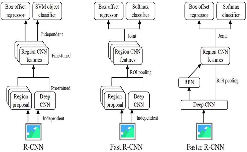
ICMAICT 2020 IOP Publishing
Journal of Physics: Conference Series 1804 (2021) 012095 doi:10.1088/1742-6596/1804/1/012095

5. DATASETS
Many image datasets have been released for training and benchmark object detection methods such as
PASCAL VOC dataset (Everingham M. et al., 2010), ImageNet dataset (Deng J. et al., 2009) and COCO
dataset (Lin T. et al., 2015). To evaluate methods in object detection, the performance metric is used
(Bashir F. et al., 2006 & Yin F. et al., 2007). The common metric used to measure the object detector
accuracy is called the mean Average Precision (mAP).

6. EVOLUTION OF CNN FOR OBJECT DETECTION
Object detection in images is one of the most direct uses of CNNs. Recognize an object in an image has
attached many challenges due to the variations that each object or the specific image could have like the
illumination or viewpoint. The meaning of object detection is recognizing and localizing objects in an
image (Zhou X. et al. 2017 & Pei T. et al., 2016).
 In 2012, Krishevsky et al. demonstrated significant performance gains on the ImageNet classification
task using a CNN (Krizhevsky A. et al., 2012), and afterward many successes could be achieved for
object detection with CNN. Different methods of object detection that uses CNNs are discussed and
compared in the following subsections.

6.1. Region-based CNN (R-CNN)
Girshick et al. proposed R-CNN method (Girshick R. et al., 2014) achieves a great accuracy of object
detection by using ConvNet. R-CNN forward pass computation has two stages. In the first one, the
regions of interest (ROIs) which represent a set of category-independent bounding boxes are generated.
These bounding boxes have a high likelihood of containing an interesting object. The region generation
proposal methods like selective search, in which the neighboring pixels with the same color or intensity
are combined to generate an object proposal, are used for generating these ROIs. There are two popular
methods: Selective search and EdgeBoxes .
 The features from each region proposal are extracted by using a convolutional network. The sub-
image within each proposal is warped to get the required size of CNN input and then fed to the
convolution neural network. After that the extraction features are input to support vector machines
(SVM) in which the final classification is provided. Figure 9 describes the R-CNN stages.
 R-CNN has several disadvantages: (1) the training is very slow due to multiple stage pipeline training
(beginning with a ConvNet for feature extraction is trained, after that the SVMs for classification are
learnt and finally a bounding box regressor is training). (2) slow speed of object detection because during
test time, feature extraction from each object proposal in all test images is done. (3) feature extraction
from each object proposal in each image required many space of storage (Girshick R. et al., 2014 & Wu
T. et al., 2017). Table 1 shows mAP that is achieved by the best R-CNNs models.
 CNN Label 1

 Label 2

 Label 3

 Input image Extract region Warped region Compute CNN Classification
 proposals features

 Figure 9 R-CNN Stages (Girshick R. et al., 2014)

 Table 1 Mean average precision (%) of (R-CNN) models.

 9

ICMAICT 2020 IOP Publishing
Journal of Physics: Conference Series 1804 (2021) 012095 doi:10.1088/1742-6596/1804/1/012095

6.2. Fast R-CNN
Fast R-CNN (Girshick R., 2015) was introduced by Girshick in 2015 to reduce the time and
computational cost spent on the R-CNN detection network, and its use enabled this algorithm to achieve
near real-time detection rates if the time spent on region proposals is ignored. Fast R-CNN enables an
end-to-end detector combining all models into a single network. In other words, the Fast R-CNN
framework trains a CNN, a classifier and a bounding box regressor in a unique model, while previously,
for example on R-CNN, a different model was used to extract features from the input image by using a
CNN, to classify with an SVM and other to predict the bounding boxes. The Fast R-CNN architecture
has some particularities starting in the input requirements taking, as usual on a ConvNet, an image and
respective object annotations but in addition a set of object proposals representing the regions of interest
(RoIs) of the images that will be used during the RoI pooling layer. Primarily the entire image is
processed with multiple convolutional and pooling layers to produce a convolutional feature map. This
first operation is one of the gains, in terms of velocity, that Fast R-CNN achieves when compared with
R-CNN because instead of running a CNN for each region of interest, it runs a single CNN for the entire
image producing at the end the mentioned feature map. After the first stage is completed, the second
stage of the framework begins, where for each object proposal a RoI pooling layer, using max pooling,
gets a small fixed size vector from the feature map. Then by a sequence of FC layers, it is mapped to a
feature vector that finally splits into two output vectors per RoI: one for the classifier (usually softmax)
to estimate the probability of each object class, while the other one with the bounding box regressor that
outputs the coordinates for each object class. Figure 10 shows the Fast R-CNN architecture.
 For each ROI Outputs:

 softmax
 FC

 Deep ROI
 ConvNet pooling FCs
 layer
 ROI
 Bbox
 projection regressor
 FC
 Input image Conv ROI feature
 feature map vector

 Figure 10 Fast R-CNN stages (Girshick R., 2015)

 The drawback of Fast R-CNN is similar to that of R-CNN that uses traditional region generation
proposal techniques such as selective search and EdgesBoxes. These become a performance bottleneck
because they are computationally expensive (Girshick R., 2015 & Jiang H. et al., 2017). The mAP scores
of the best Fast R-CNNs are shown in Table 2.

 Table 2 Mean average precision (%) of (Fast R-CNN) models.

6.3. Faster R-CNN
Faster R-CNN, introduced by Microsoft Research in 2016 (Ren S. et al., 2016), is a ConvNet based
method and it has shown very good results in object detection tasks. In this framework, the Region
Proposal Networks (RPN) is introduced.
 A separate region proposal network (RPN) is used for detecting regions from an input image that
most likely contain objects. These region proposals are fed to detection network, to make the final
decision about object existence and bounding boxes. The important thing is that the computations will
be more efficient because RPN shares convolutional layers with the object detection network. It creates

 10

ICMAICT 2020 IOP Publishing
Journal of Physics: Conference Series 1804 (2021) 012095 doi:10.1088/1742-6596/1804/1/012095

multiple region proposals that have different scales and aspect ratios by looking at both objectness scores
and map positions. RPN combined with Fast R-CNN in Faster R-CNN model is considerably faster than
the Selective search method combined with R-CNN and Fast R-CNN. Faster R-CNN architecture
merges both object detection and recognition computations back into one using a concept of Region
Proposal Network which is a small extension of original recognition network. The RPN is put before
last pooling layer and consists of convolutional layer of size 33 (where width dimension is equal to
width of preceding layer) and feeds the output of this layer into 2 layers: box-regression (reg) layer and
box-classification (cls) layer which are both implemented as a convolutional layer of dimension11 as
illustrated in Figure 11(a). The reg and cls layers outputs 4k and 2k dimensional vectors respectively,
where k stands for number of so called anchors at the processed position. Each anchor stands for a
different setting of scales and aspect ratios at which RPN is analyzing given position. By default three
different scales and three different aspect ratios are used resulting in k=9. This approach ensures
translational invariance of anchors. Reg layer estimates regression of possible bounding box of an object
and cls layer computes 2 probabilities (object or not-object) in each anchor at a given position. Outputs
of this RPN network are then fed into Fast R-CNN part of networks as shown in Figure 11(b), which
expects RoI proposals and feature maps of last convolutional layer and applies so called RoI pooling
effectively replacing last max pooling layer. RoI pooling divides each region of RoI proposal of
dimension wh into grid of size WH where W and H are parameters of a layer and performing classical
max pooling on each cell of size w/Wh/H effectively squashing features of any RoI into fixed length
vector of size WH. This RoI pooled vector is then fed into usual FC layers where the output at the end
actually consists of two different output layers, one computing probability of a given class and the other
one estimating positions of bounding box depending on found class (Ren S. et al., 2016 & Eggert C.et
al., 2017 & Lee C. et al., 2016). The mAP that is obtained by the best Faster R-CNNs are shown in Table
3.
 Table 3 Mean average precision (%) of (Faster R-CNN) models.

The model designs of R-CNN, Fast R-CNN and Faster R-CNN are illustrated by comparing the
differences in Figure 12.
 2k scores 4k coordinates k anchor boxes RPN
 2-class
 cls layer reg layer softmax

 256-d bbox
 Sliding window
 intermediate layer
 l

 Feature
 CNN
 maps

 Input image multi-class
 Sliding window  softmax
 
 
 conv feature map bbox
 Fast R-CNN

 (a (b
 Figure 11 (a) Region Proposal Network (b) Faster R-CNN stages

 11

ICMAICT 2020 IOP Publishing
Journal of Physics: Conference Series 1804 (2021) 012095 doi:10.1088/1742-6596/1804/1/012095

Figure 12 Summary of methods in the R-CNN family

6.4. You Only Look Once (YOLO):
Another object detection framework called (YOLO) is proposed by Redmon et al in 2016 (Redmon J.
et al., 2016) to use features from the entire image to predict object bounding box instead of sliding
windows on the last convolutional feature maps. Only one neural network is used to process the entire
image. This network splits image into blocks (regions) to predict bounding boxes and probabilities for
each block (region). The predicted probabilities are used to weight these bounding boxes. The YOLO
architecture in simple terms consists of an SS grid cells of classifiers and regressors. Each grid cell
consists of bounding box regression and classification heads that share the same convolutional features.
Each grid has B bounding box regression heads that predicts a bounding box each with 5 values x, y, w,
h and confidence of an object being there. Where (x, y) is the center of the bounding box relative to the
grid cell. Each grid cell also contains a classifier which predicts C conditional class probabilities as well.
So the overall final output from a YOLO network is tensor of size: SS(5*B+C).
 In other word, each grid cell is considered as a standalone system specifically focusing on a smaller
region within the input image with B regression heads, each predicting a bounding box and a confidence
which at training time must equal the intersection over union (IOU) between the predicted box and the
ground truth box if the object is present, otherwise IOU is zero. Thus in YOLO the
confidence predicted by each regression head is defined as Pr(object)*IOU . Then within each grid there
is also a classifier head that predicts C conditional probabilities per class Pr(classiobject). So Baye’s
rule is used to get equation (15):
 Pr | ∗ Pr ∗ ∗ (15)
 The overall confidence score encodes the class probabilities and how well the predicted
box fits the object. Low confidence detections can then be thresholded out leaving the strong
detections. Since neighboring grid cells will also be activated, this will result in
multiple bounding boxes around a single object. So non-maxima suppression is applied in order
to keep the strongest detection around a single object. So the speedup comes about because this
is purely feedforward whereby the system outputs SSB bounding
boxes and SSC confidence scores in one glance hence “you only look once”. This is faster
than running a regional proposal network (RPN) to get p proposals and then running
classification phase on each of the p proposals as done in other techniques. It is also faster than
methods that use a sliding window technique to scan an image at multiple locations (Redmon
J. et al., 2016 & Javad M. et al., 2017 & Ren P. et al., 2017).
 The drawback of YOLO Compared with Faster R-CNN that YOLO is less accurate. The
mAP scores of YOLO model are shown in Table 4.

 12

ICMAICT 2020 IOP Publishing
Journal of Physics: Conference Series 1804 (2021) 012095 doi:10.1088/1742-6596/1804/1/012095

 Table 4 Mean average precision (%) of (YOLO) models.

6.5. Single-Shot-Multibox-Detector (SSD)
The extension of the YOLO method is Single Shot Multibox Detector (SSD) network by W. Liu et al.
(2016) (Liu W. et al., 2016). The SSD network also predicts bounding boxes and classication in one
single feed forward but extents it with a hypercolumn approach. The hypercolumn approach is used to
combine multiple feature maps to detect objects of various sizes. The SSD network is called single shot
since both object localisation and classication are done within a single feed forward through the network.
 The network is a fully convolutional network; therefore it can be used for images with any resolution.
Two architectures are proposed in the original paper: SSD512 architecture for an input resolution of 512
x 512 pixels and SSD300 for an input resolution of 300 x 300 pixels.
 The input image passes through many convolutional layers with filters of different sizes.
After that, a 3x3 sized convolutional filter is applied on the feature map to produce a bounding
boxes set that is similar to the anchor boxes of Fast R-CNN.
 Finally, non-maximum suppression method is used to collect overlapping bounding boxes
together into one box. Non-maximum suppression looks through the boxes that contains the
same object to produce the final detections by keeping the one with the highest confidence and
discarding the others.
 The best SSD models have mAP score as shown in Table 5. This method has much worse
performance for small objects.

 Table 5 Mean average precision (%) of (SSD) models.

7. COMMON CONVENT ARCHTICTURES
Despite the fact that ConvNet history goes back to 1980s (Rumelhart D. et al., 1985), it has been in
recent years when ConvNets have gained popularity in computer vision tasks, mainly due to availability
of computational resources.

7.1. LeNet
ConvNet was in back in 1998 when the first successful ConvNet application was developed. It was
called LeNet (LeCun Y. et al., 1998) and it could classify handwritten digits. LeNet had two stacked
convolutional layers, followed by 3 FC layers. After each convolutional layer there was pooling layer.
LeNet had 340K connection and only 60K parameters because of weight sharing.

7.2. AlexNet
ConvNets became popular much later, in 2012, when AlexNet (Krizhevsky A. et al., 2012) was
introduced. AlexNet could classify images on different categories and it won ILSVRC 2012 competition
by a significant margin to the second contestant. AlexNet had deeper and spatially larger network
architecture than LeNet. It had five stacked convolutional layers, followed by three FC layers. In
addition, three pooling layers followed each of the first, second and fifth convolutional layer. The

 13

ICMAICT 2020 IOP Publishing
Journal of Physics: Conference Series 1804 (2021) 012095 doi:10.1088/1742-6596/1804/1/012095

architecture of AlexNet is illustrated in Figure 13(a). The stride on the first convolutional layer is 4. All
other convolutional layers have stride of 1. All pooling use 33 kernel and stride of 2. The last layer
outputs class probabilities for 1000 categories. AlexNet had 60M parameters. ZF Net in 2013 (Zeiler M.
et al., 2014) was an improvement to AlexNet. It had similar architecture, only difference is filter size
and stride that were smaller in the first convolutional layer. Because of this, the first and second
convolutional layer retained much more information, which in turn improved classification
performance.

7.3. VGG Net
VGG Net (Simonyan K. et al, 2015), introduced in 2014 by Simonyan and Zisserman, showed that by
using very small convolution filters (3  3) and pushing the depth of the network to 16-19 layers (see
Figure 13(b)), a significant improvement on the prior architectures could be achieved on image
recognition tasks. VGG Net placed second in the ILSVRC 2014 image recognition challenge. Since
then, VGG Net has been used successfully also in object detection, most importantly in Fast R-CNN
(Girshick R., 2015) and Faster R-CNN (Ren S. et al., 2016).

7.4. GoogleNet
GoogleNet (Szegedy C. et al, 2015), introduced by Szegedy et al., ranked first in the ILSVRC 2014
image recognition challenge. GoogleNet presented a new ConvNet architecture, where the network
consisted of Inception Modules. The key idea of Inception Module is to feed the input data
simultaneously to several convolutional layers and then concatenate outputs of each layer into a single
output. Each convolutional layer has a different filter size and they produce spatially equal sized outputs.
Because of this, a single Inception Module can process information at various scales simultaneously,
thus leading to better performance. An Inception Module can also have a pooling layer side by side with
convolutional layers. In order to avoid computational blow up, Inception Modules utilize 11
convolutional layers for dimension reduction. A typical Inception Module is described in Figure 13(c).
There are 3 convolutional layers with filter sizes 11, 33 and 55, in addition to one pooling layer with
filter size 33. Dashed volumes are 11 convolutions implementing dimension reduction. Stride of 1 is
used in every layer. The main benefit of this architecture is that both the depth and width of the network
are increased, while keeping computational complexity in control. GoogleNet have 5M parameters
(AlexNet 60M). Since introducing it, a few follow-up versions with performance improvements have
been proposed (Szegedy C. et al., 2016 & Ioffe S. et al., 2016).

 Figure 13 The architecture of (a) AlexNet (b) 16 layer VGG Net (c) a typical Inception Module

 14

ICMAICT 2020 IOP Publishing
Journal of Physics: Conference Series 1804 (2021) 012095 doi:10.1088/1742-6596/1804/1/012095

7.5. Residual Network
In 2015, He et al. introduced the Residual Network (ResNet) architecture (He K. et al., 2016), which
won the ILSVRC 2015 on image recognition. They replaced traditional stacking convolutional layers
with Residual Modules. In a single Residual Module, a couple of stacking convolutional layers is
bypassed with a skip connection. The output of the skip connection is then added to the output of the
stacking layers. Every convolutional layer in a Residual Module utilizes Batch Normalization (Ioffe S.
et al., 2015) to cope with internal covariate shift. ReLU (Nair V. et al. 2010 & Glorot X. et al. 2011) is
used for non-linearity. Two different Residual Modules, basic and bottleneck, were proposed by the
authors that is described in Figure 14. Residual Module keeps the spatial size unchanged. The purpose
of 11 convolutions in bottleneck Residual Module, before and after 33 convolution, is to reduce and
then increase (restore) dimensions, leaving the 33 layer a bottleneck with smaller input/output
dimensions.
 A typical ResNet architecture consists of a great number of stacked Residual Modules, making the
network much deeper (from tens to hundreds of layers) compared to traditional networks. The authors
of ResNet demonstrate that it is easier to optimize a very deep Residual Network than its counterpart, a
traditional network with stacking layers. With Residual Networks, the training error is much lower when
the depth increases, which in turns gives accuracy improvements. Since introducing the Residual
Network architecture, several improvements have been proposed. The authors, He et al., introduced a
new Residual Module, which further makes training easier and improves generalization (He K. et al.,
2016). Zagoruyko and Komodakis argued that very deep ResNet architectures are not needed for state-
of-the-art performance (Zagoruyko S. & Komodakis N., 2016). They decreased the depth of the network
and increased the size of a Residual Module by adding more features and convolutional layers. Their
Wide Residual Network trains faster and it outperformed previous ResNet architectures on CIFAR-10
and CIFAR-100 datasets by a distinct margin. Currently, ResNets are state-of-the-art ConvNet models
and they have been shown to perform remarkable well both in image recognition and human pose
estimation tasks.

 Figure 14 The architectures of (a) basic and (b) bottleneck Residual Modules

8. CONCLUSION
Convolution Neural Networks (ConvNets or CNNs) significantly enhances the capabilities of the
feedforward network such as MLP by inserting convolution layers. As seen, the two main advantages
of Convolution Neural Networks are: (a) parameter sharing which is reduced the computation cost and
the network complexity. (b) sparsity of connection which helps in training with smaller training sets
since each output value depends only on a small number of inputs that makes CNN translation
invariance. CNNs are the basis of all modern computer vision models. Many perceptual tasks have been
performed with help of CNNs such as handwriting recognition, traffic sign recognition, pedestrian
detection, human action recognition, object recognition, Scene parsing, Breast cancer cell mitosis
detection, etc. In this paper, many methods of object detection were discussed based on their advantages
and disadvantages. Table 6 summarizes the comparison in performance and speed between these
detection methods on PASCAL VOC 2007.

 15

ICMAICT 2020 IOP Publishing
Journal of Physics: Conference Series 1804 (2021) 012095 doi:10.1088/1742-6596/1804/1/012095

 Table 6 Detection frameworks on PASCAL VOC 2007

References
[1] Akhtar N. & Mian A., 2018. Threat of Adversarial Attacks on Deep Learning in ComputerVision:
 A Survey. IEEE Access. :14410-14430.
[2] Bashir F. & Porikli F., 2006. Performance Evaluation of Object Detection and Tracking Systems.
 Proceedings of the 9th IEEE International Workshop on Visual Surveillance and Performance
 Evaluation of Tracking and Surveillance (VS-PETS 06).
[3] Deng J., Dong W., Socher R., Li L., Li K. & Fei-Fei L., 2009. ImageNet: A Large-Scale
 Hierarchical Image Database. IEEE: Computer Vision and Pattern Recognition (CVPR). :248-
 255.
[4] Dumoulin V. & Visin F., 2018. A Guide to Convolution Arithmetic for Deep Learning.
 arXiv:1603.07285v2.
[5] Eggert C., Brehm S., Winschel A., Zecha D. & Lienhart R., 2017. A Closer Look: Small Object
 Detection in Faster R-CNN. Proceedings of the IEEE international conference on Multimedia
 and Expo (ICME). :421-426.
[6] Everingham M., Van Gool L., Williams C., Winn J. & Zisserman A., 2010. The PASCAL Visual
 Object Classes (VOC) Challenge. International Journal of Computer Vision. Springer. 88:
 303-338.
[7] Gheisari M., Wang G. & Bhuiyan M., 2017. A Survey on Deep Learning in Big Data. Proceedings
 of the IEEE International Conference on Computational Science and Engineering (CSE) and
 IEEE International Conference on Embedded and Ubiquitous Computing (EUC). :173-180.
[8] Girshick R., 2015. Fast r-cnn. Proceedings of the IEEE International Conference on Computer
 Vision (ICCV). :1440–1448.
[9] Girshick R., Donahue J., Darrell T. & Malik J., 2014. Rich Feature Hierarchies for Accurate
 Object Detection and Semantic Segmentation. Proceedings of the IEEE Conference on
 Computer vision an Pattern Recognition. :580-587.
[10] Glorot X., Bordes A. & Bengio Y., 2011. Deep sparse rectifier neural networks. Proceedings of
 the International Conference on Artificial Intelligence and Statistics (AISTATS). :315–323.
[11] He K., Zhang X., Ren S. & Sun J., 2016. Identity Mappings in Deep Residual Networks.
 arXiv:1603.05027.
[12] He K., Zhang X., Ren S. & Sun J., 2016. Deep residual learning for image recognition.
 Proceedings of the IEEE Conference on Computer Vision and Pattern Recognition (CVPR).
 :770-778.
[13] Ioffe S. & Szegedy C., 2015. Batch Normalization: Accelerating Deep Network Training by
 Reducing Internal Covariate Shift. arXiv:1502.03167.
[14] Ioffe S., Szegedy C. & Vanhoucke V., 2016. Inception-v4, Inception-resnet and The Impact of
 Residual Connections on Learning. arXiv:1602.0726.
[15] Javad M., Brendan C., Li F. & Alexander C., 2017. Fast YOLO: A Fast You Only Look Once
 System for Real-time Embedded Object Detection in Video. arXiv:1709.05943v1.
[16] Jiang H. & Learned-Miller E., 2017. Face Detection with the Faster R-CNN. Proceedings of the

 16

ICMAICT 2020 IOP Publishing
Journal of Physics: Conference Series 1804 (2021) 012095 doi:10.1088/1742-6596/1804/1/012095

 12th International Conference on Automatic Face & Gesture Recognition. :650-657.
[17] Kao Y. & Venkatachalam R., 2018. Human and Machine Learning. Springer. :1-21.
[18] Koohzadi M. & Moghadam N., 2017. Survey on Deep Learning Methods in Human Action
 Recognition. IET Computer Vision. 11: 623-632.
[19] Krebs S., Duraisamy B. & Flohr F., 2017. A survey on Leveraging Deep Neural Networks for
 Object Tracking. Proceedings of the 20th IEEE International Conference on Intelligent
 Transportation Systems (ITSC). :411-418.
[20] Krizhevsky A., Sutskever I. & Hinton G.E., 2012. Imagenet Classification with Deep
 Convolutional Neural Networks. Advances in Neural Information Processing Systems (NIPS).
 :1097–1105.
[21] LeCun Y., Bengi Y. & Hinton G., 2015. Deep learning. NAUTRE. 521: 436-444.
[22] LeCun Y., Bottou L., Bengio Y. & Haffner P., 1998. Gradient-Based Learning Applied to
 Document Recognition. IEEE. 86: 2278-2324.
[23] Lee C., Kim H. & Won K., 2016. Comparison of Faster R-CNN Models for Object Detection.
 Proceedings of the 16th IEEE International Conference on Control Automation and Systems
 (ICCAS) :107-110.
[24] Liu T., Fang Sh., Zhao Y., Wang P. & Zhang J., 2015. Implementation of Training Convolutional
 Neural Networks. arXiv:1506.01195.
[25] Lin T., Maire M., Belongie S., Bourdev L. & Girshick R., 2015. Microsoft COCO: Common
 Objects in Context. arXiv:1405.0312v3.
[26] Liu W., Anguelov D., Erhan D., Szegedy Ch., Reed S., Fu Ch. & Alexander C., 2016. SSD: Single
 Shot MultiBox Detector. arXiv:1512.02325v5.
[27] Mohammadi M. & Sorour S., 2017. Deep Learning for IoT Big Data and Streaming Analytics: A
 Survey. arXiv:1712.04301v1.
[28] Nair V. & Hinton G., 2010. Rectified Linear Units Improve Restricted Boltzmann Machines.
 Proceedings of the International Conference on Machine Learning (ICML) :807–814.
[29] Neena A. & Geetha M., 2017. A Review on Deep Convolution Neural Networks. IEEE Advanced
 Technology for Humanity. :588-592.
[30] Pei T. & Xiaoyu W., 2016. Object Proposals Detection. Proceedings of the IEEE Conference on
 Computer and Communication. :445-448.
[31] Pratt H., Coenen F., Broadbent D., Harding S. & Zheng Y., 2016. Convolutional Neural Networks
 for Diabetic Retinopathy. ELSEVIER, Procedia Computer Science. :200 – 205.
[32] Redmon J., Divvala S., Girshick R. & Farhadi A., 2016. You Only Look Once: Unified, Real-
 Time Object Detectio. Proceedings of the IEEE Conference on Computer Vision and Pattern
 Recognition (CVPR). :779-788.
[33] Ren P., Fang W. & Djahel S., 2017. A Novel YOLO-based Real-time People Counting Approach.
 Proceedings of the IEEE International Smart Cities Conference (ISC2). :1-2.
[34] Ren S., He K., Girshick R. & Sun J., 2016. Faster r-cnn: Towards real-time object detection with
 region proposal networks. Advances in Neural Information Processing Systems (NIPS). :91–
 99.
[35] Rumelhart D., Hinton G. & Williams R., 1985. Learning Internal Representations by Error
 Propagation. Tech. rep., DTIC Document.
[36] Simonyan K. & Zisserman A., 2015. Very deep convolutional networks for large-scale image
 recognition. arXiv:1409.1556.
[37] Srivastava N., Hinton G.E., Krizhevsky A. & Sutskever I., Salakhutdinov R., 2014. Dropout: A
 Simple Way to Prevent Neural Networks from Overfitting. Journal of Machine Learning
 Research (JMLR). :1929–1958.
[38] Szegedy C., Liu W., Jia Y., Sermanet P., Reed S., Anguelov D., Erhan D., Vanhoucke V. &
 Rabinovich A., 2015. Going deeper with convolutions. Proceeding of the IEEE Conference on
 Computer Vision and Pattern Recognition (CVPR). :1-9.
[39] Szegedy C., Vanhoucke V., Ioffe S. , Shlens J. & Wojna Z., 2016. Rethinking The Inception

 17

ICMAICT 2020 IOP Publishing
Journal of Physics: Conference Series 1804 (2021) 012095 doi:10.1088/1742-6596/1804/1/012095

 Architecture for Computer Vision. arXiv:1512.00567.
[40] Wei B., Sun X., Ren X. & Xu J., 2017. Minimal Effort Back Propagation for Convolutional
 Neural Network. arXiv:1709.05804v1.
[41] Wu T., Li X., Song X., Sun W., Dong L. & Li B., 2017. Interpretable R-CNN.
 arXiv:1711.05226v1.
[42] Yan Z. & Sean Zhou X., 2017. How Intelligent are Convolutional Neural Networks?.
 arXiv:1709.06126v2.
[43] Yin F., Makris D. & Velastin S., 2007. Performance Evaluation of Object Tracking Algorithms.
 Proceedings of the 10th IEEE International Workshop on Performance Evaluation of Tracking
 and Surveillance (PETS2007).
[44] Yu K. & Salzmann M., 2017. Second-order Convolutional Neural Networks.
 arXiv:1703.06817v1.
[45] Zagoruyko S. & Komodakis N., 2016. Wide Residual Networks. arXiv:1605.07146v4.
[46] Zeiler M. & Fergus R., 2014. Visualizing and understanding convolutional networks.
 Arxiv:1311.2901.
[47] Zhi-Peng F. & Yan-Ning Z., 2014. Survey of Deep Learning in Face Recognition. Proceedings
 of the IEEE International Conference on Orange Technologies. :5-8.
[48] Zhou X., Gong W., Fu W. & Du F., 2017. Application of Deep Learning in Object Detection.
 Proceedings of the 16th International Conference on Computer and Information Science
 (ICIS). :631-634.

 18