Accelerating Convolutional Networks via Global & Dynamic Filter Pruning - IJCAI
←
→
Page content transcription
If your browser does not render page correctly, please read the page content below
Proceedings of the Twenty-Seventh International Joint Conference on Artificial Intelligence (IJCAI-18)

         Accelerating Convolutional Networks via Global & Dynamic Filter Pruning

    Shaohui Lin1,2 , Rongrong Ji1,2∗ , Yuchao Li1,2 , Yongjian Wu3 , Feiyue Huang3 , Baochang Zhang4
       1
         Fujian Key Laboratory of Sensing and Computing for Smart City, Xiamen University, China
                2
                  School of Information Science and Engineering, Xiamen University, China
                        3
                          BestImage, Tencent Technology (Shanghai) Co.,Ltd, China
           4
             School of Automation Science and Electrical Engineering, Beihang University, China
                                      Contact author: rrji@xmu.edu.cn

                               Abstract                                     CNNs in real-time applications without the support of highly-
                                                                            efficient Graphic Processing Units (GPUs). As a result, the
        Accelerating convolutional neural networks has                      acceleration of convolutional networks has become emerging.
        recently received ever-increasing research focus.
                                                                               Recent works in convolutional neural network acceleration
        Among various approaches proposed in the litera-
                                                                            can be categorized into three groups, i.e., low-rank decompo-
        ture, filter pruning has been regarded as a promising
                                                                            sition, parameter quantization, and network pruning. Among
        solution, which is due to its advantage in significant
                                                                            them, network pruning has received ever-increasing research
        speedup and memory reduction of both network
                                                                            focus, which merits in limited memory footprints due to the
        model and intermediate feature maps. To this end,
                                                                            small amount of filter parameters and intermediate activation,
        most approaches tend to prune filters in a layer-
                                                                            which is highly required for memory-light online inference.
        wise fixed manner, which is incapable to dynami-
                                                                            Methods in network pruning can be further categorized into
        cally recover the previously removed filter, as well
                                                                            either non-structured or structured pruning. Non-structured
        as jointly optimize the pruned network across lay-
                                                                            pruning [LeCun et al., 1989; Hassibi and Stork, 1993; Han
        ers. In this paper, we propose a novel global & dy-
                                                                            et al., 2015a; 2015b] targets at directly pruning parameters
        namic pruning (GDP) scheme to prune redundant
                                                                            independently in each layer, which will cause irregular mem-
        filters for CNN acceleration. In particular, GDP
                                                                            ory access that adversely impacts the efficiency of online in-
        first globally prunes the unsalient filters across all
                                                                            ference. Under such a circumstance, specialized hardware
        layers by proposing a global discriminative func-                   [Han et al., 2016] or software [Liu et al., 2015; Park et al.,
        tion based on prior knowledge of each filter. Sec-
                                                                            2017] designs are required to further speedup the pruned
        ond, it dynamically updates the filter saliency all
                                                                            unstructured CNNs. Instead, structured pruning [Anwar et
        over the pruned sparse network, and then recov-
                                                                            al., 2015; Lebedev and Lempitsky, 2016; Wen et al., 2016;
        ers the mistakenly pruned filter, followed by a re-
                                                                            Li et al., 2016; Luo et al., 2017; Molchanov et al., 2017;
        training phase to improve the model accuracy. Spe-
                                                                            Hu et al., 2016] aims at directly removing filters as a whole,
        cially, we effectively solve the corresponding non-
                                                                            which is far more efficient and independent to specialized
        convex optimization problem of the proposed GDP
                                                                            hardware/software platforms. For instance, Anwar et al. [An-
        via stochastic gradient descent with greedy alter-
                                                                            war et al., 2015] introduced the structured sparsity to ei-
        native updating. Extensive experiments show that
                                                                            ther filter-wise or channel-wise convolutional filter selection,
        the proposed approach achieves superior perfor-
                                                                            based on which pruned filters with regularity by using parti-
        mance to accelerate several cutting-edge CNNs on
                                                                            cle filtering. Luo et al. [Luo et al., 2017] implicitly associ-
        the ILSVRC 2012 benchmark, comparing to the
                                                                            ated the convolutional filter in the current layer with the input
        state-of-the-art filter pruning methods.
                                                                            channel in the next layer, based on which pruned filters in the
                                                                            current layer via input channel selection of the next layer.
1       Introduction                                                           However, the existing structured pruning schemes prune
                                                                            the convolutional neural network in a layer-by-layer fixed
Convolutional neural networks (CNNs) have achieved re-
                                                                            manner, which is less adaptive, less efficient, and less effec-
markable success in various applications such as image clas-
                                                                            tive. First, in local pruning, iterative layer-wise pruning and
sification [He et al., 2016; Krizhevsky et al., 2012; Simonyan
                                                                            local fine-tuning are required, which is computational inten-
and Zisserman, 2014], object detection [Girshick et al., 2014]
                                                                            sive. Second, mistaken pruning of the salient filter is irre-
and semantic segmentation [Long et al., 2015]. However, the
                                                                            trievable, which is inadaptive and the pruned network cannot
promising performance is accompanied by significant com-
                                                                            achieve an optimal performance.
putation cost, which raises huge difficulty to deploy these
                                                                               In this paper, we present a novel global & dynamic prun-
    ∗
        Corresponding author                                                ing (GDP) scheme to prune redundant filters to address above

                                                                     2425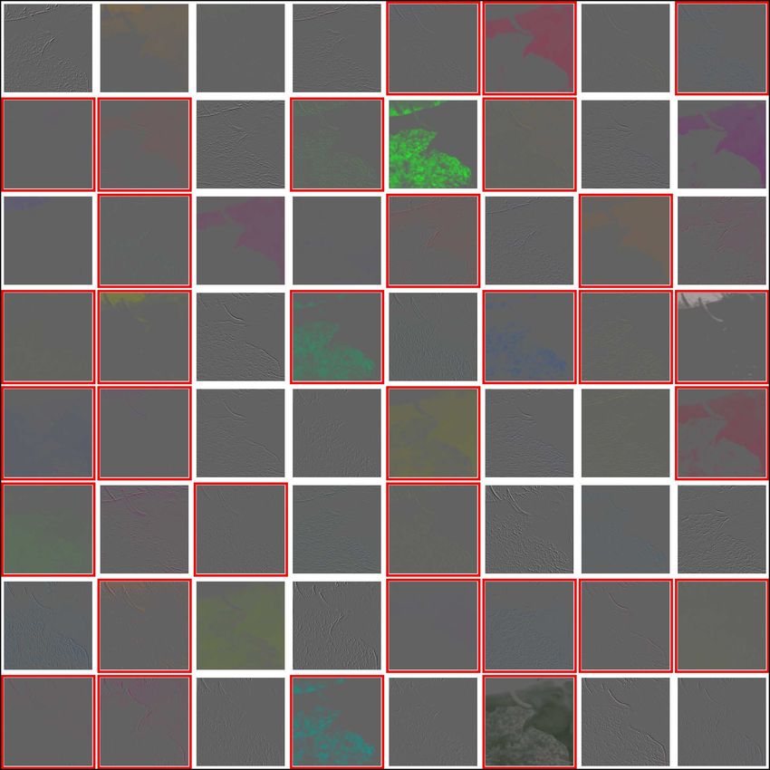
Proceedings of the Twenty-Seventh International Joint Conference on Artificial Intelligence (IJCAI-18)
              Output
FC layers                                                                                                               unimportant weights, which is determined by the second-
                      …   Pre-trained model               Intermediate              Update Parameters W*
                           with full masks                 parameters                  and reselect m                   order derivative matrix of the loss function with respect to the
                                                Global                         Dynamic                                  parameters. Recently, Han et al. [Han et al., 2015a; 2015b]
Conv Layers

                                               Pruning                         updating
                                                                                                                        proposed to prune parameters by using iterative thresholding
                  …

                                           …                               …                               …
                                                                                                                        to remove unsalient weights with small absolute values. Guo
                                                                                                                        et al. [Guo et al., 2016] pruned weights by using connection
                              …   ⊙        …                 …   ⊙     …                           ⊙
                                                                                                                        splicing to avoid incorrect pruning. However, such scheme
                                                                                               …           …
                             W*        m                    W*        m                       W*       m
Input

                                                                                                                        can only be worked in a local manner layer-by-layer. Differ-
              …

                                                                                                           1 0
                             Filters W*:       …         ⊙ : Khatri-Rao product           Global mask m:
                                                                                                                        ent from connection splicing, the proposed dynamic updating
Figure 1: An illustration of GDP. Each rectangle with color (e.g.,                                                      is conducted in a global manner, which can restore important
red rectangle) is a filter in the filter set W∗ , while a global mask                                                   filters that were mistakenly removed across all layers.
m with binary values determines the saliency of filters (i.e.,  indi-                                                      In line with our work, a few methods have been pro-
cates the corresponding filter is salient, and  is unsalient). First, a                                                posed for filter-level/channel pruning (i.e., structured prun-
pre-trained model and a full global mask are employed to initialize                                                     ing), which can reduce both network size and inference speed.
the network. Then, the redundant filters are globally pruned across                                                     Li et al. [Li et al., 2016] measured the importance of each
all layers by masking out the corresponding value as 0. Finally, it-                                                    filter by calculating the `1 -norm to prune unsalient filters to-
eratively dynamic updating of filters and global mask is done to im-
prove the accuracy of the pruned network. (Best viewed in color.)
                                                                                                                        gether with their corresponding feature maps. Hu et al. [Hu et
                                                                                                                        al., 2016] computed the Average Percentage of Zeros (APoZ)
                                                                                                                        of each filter, i.e., the percentage of zero values in the output
two issues, which can largely accelerate the pruned networks                                                            feature map associated with the corresponding filter, which
while reducing the networks accuracy loss. Unlike the pre-                                                              serves as its score to guide pruning. Lebedev et al. [Lebe-
vious schemes of layer-by-layer fixed filter pruning, our key                                                           dev and Lempitsky, 2016] and Wen et al. [Wen et al., 2016]
innovation lies in evaluating the importance/saliency of indi-                                                          utilized group sparsity regularization to prune convolutional
vidual filter globally across all network layers, upon which                                                            filters in a group-wise fashion during the training, which is
dynamically and iteratively prune and tune the network, with                                                            however less efficient since only stochastic gradient descend
the mechanism to recall filters that are mistakenly pruned in                                                           is used. Recently, a new criterion based on Taylor expan-
the previous iterations. Figure 1 demonstrates the flowchart                                                            sion has been introduced in [Molchanov et al., 2017] to glob-
of the proposed framework. In particular, we first initialize                                                           ally prune one filter and then fine-tune the pruned network.
a pre-trained convolutional network and globally mask all fil-                                                          However, it was prohibitively costly when applying to deep
ters to be equal to 1 (i.e., an external switch which determines                                                        networks, as time-consuming fine-tuning has to be done after
whether the filter is pruned). Then, we design a global dis-                                                            pruning each filter. Our method is different to all above meth-
criminative function to determine the saliency scores of indi-                                                          ods, in terms of globally removing unsalient filters across
vidual filters. Such scores guide us to globally prune the un-                                                          all layers, as well as dynamically restoring salient filters that
salient filters across all layers, which equivalently masks out                                                         were previously mislabeled removed.
unsalient filters as 0. Finally, we iteratively tune the sparse                                                             Orthogonal methods to our work include low-rank de-
network and dynamically update the filter saliency in a top-                                                            composition [Denton et al., 2014; Jaderberg et al., 2014;
down manner. By such operations, filters that are previously                                                            Lin et al., 2016; 2017; Lebedev et al., 2014; Kim et al., 2015],
masked out is possible to recalled, which significantly im-                                                             parameter quantization [Gong et al., 2014; Wu et al., 2016;
proves the accuracy of the pruned network. In terms of op-                                                              Courbariaux et al., 2015; Courbariaux and Bengio, 2016;
timization, GDP can be described as a non-convex optimiza-                                                              Rastegari et al., 2016], which have also widely used to ac-
tion problem, which is then effectively solved via the stochas-                                                         celerate convolutional networks. Low-rank decomposition
tic gradient descent with greedy alternative updating.                                                                  [Denton et al., 2014; Jaderberg et al., 2014; Lin et al., 2017;
   The proposed GDP is evaluated on the ImageNet 2012                                                                   Lebedev et al., 2014; Kim et al., 2015] typically decomposed
dataset [Russakovsky et al., 2015] and implemented on the                                                               convolutional filters into a sequence of tensor based convo-
widely-used AlexNet [Krizhevsky et al., 2012], VGG-16 [Si-                                                              lutions with fewer parameters. For parameter quantization,
monyan and Zisserman, 2014] and ResNet-50 [He et al.,                                                                   Gong et al. [Gong et al., 2014] and Wu et al. [Wu et al.,
2016]. Comparing to the state-of-the-art filter pruning meth-                                                           2016] employed product quantization over parameters to re-
ods [Wen et al., 2016; Li et al., 2016; Luo et al., 2017;                                                               duce the redundancy in the parameter space. Recently, di-
Molchanov et al., 2017; Hu et al., 2016], the proposed GDP                                                              rectly predicting the model with binary weights has been pro-
scheme achieves the superior performance by a factor of                                                                 posed in [Courbariaux et al., 2015; Courbariaux and Bengio,
2.12× GPU speedup with 1.15% Top-5 accuracy loss on                                                                     2016; Rastegari et al., 2016]. It is worth to note that, our
AlexNet, 2.17× CPU speedup with 1.45% Top-5 accuracy                                                                    scheme can be integrated with the above orthogonal methods
loss on VGG-16, and 1.93× CPU speedup with 2.16% Top-5                                                                  to further accelerate the pruned network.
accuracy loss on ResNet-50.
                                                                                                                        3     Globally Dynamic Pruning
2             Related Work                                                                                              3.1    Notations
LeCun et al. [LeCun et al., 1989] and Hassibi et al. [Hassibi                                                           CNN can be viewed as a feed-forward multi-layer architec-
and Stork, 1993] proposed a saliency measurement to remove                                                              ture that maps the input image to a certain output vector. In

                                                                                                                 2426
Proceedings of the Twenty-Seventh International Joint Conference on Artificial Intelligence (IJCAI-18)
                                                                                                 o
CNN, the convolutional layers are most time-consuming. Let                 Y1 , Y2 , · · · , YN , where Xi and Yi represent an input
us denote a set of image feature maps in the l-th layer by               and a target output, respectively. We propose to solve the fol-
Zl ∈ RHl ×Wl ×Cl with size Hl × Wl and individual maps                   lowing optimization problem:
(or channels) Cl . The feature maps can either be the in-
put of the network Z0 , or the output feature maps Zl with                                   min L Y, g X ; W ∗ , m
l ∈ [1, 2, · · · , L]. In addition, we denote individual feature                                                                     (4)
            (k)                                                                               s.t. m = h(W ∗ )
map by Zl ∈ RHl ×Wl with k ∈ [1, 2, · · · , Cl ]. The in-                                                    PL
dividual output feature map of the l-th convolutional layer                                         m 0 ≤ β l=1 Cl ,
  (k)                                                                    where L(·) is a loss function for the pruned network, e.g.,
Zl is obtained by applying the convolutional operator (∗)
to a set of input feature maps with filters parameterized by             cross-entropy loss. g X ; W ∗ , m takes the input X , the fil-
   (k)
Wl ∈ Rd×d×Cl−1 1 , i.e.,                                                 ters W ∗ and the global mask m to map to an s-dimensional
                                                                         output (s is the number of classes). h(·) is a global discrim-
                     (k)                 (k)                             inative function to determine the saliency values of filters,
                   Zl      = f (Zl−1 ∗ Wl ),                   (1)
                                                                         which depends on the prior knowledge of W ∗ . The output
where f (·) is a non-linear activation function, e.g., rectifier         entry of function h(·) is binary, i.e., to be 1 if the correspond-
linear unit (ReLU).                                                      ing filter is salient, and 0 otherwise.
   In many deep learning frameworks like Caffe [Jia et al.,                 Eq. 4 is the core function in our GDP framework, which is
2014] and Tensorflow [Abadi et al., 2016], the tensor-based              non-convex and whose solver will be introduced in Sec. 3.3.
convolution operator is reformulated as a matrix-by-matrix               β ∈ (0, 1] is a threshold to determine the sparsity of the
multiplication by lowering the input and reshaping the filters,          pruned network. The problem Eq. 4 is NP-hard, because of
such as:                                                                 the k · k0 operator. We simplify this NP-hard problem by
                   Z∗l = f (Z∗l−1 × Wl∗ ),                   (2)         bounding m on prior knowledge of W ∗ . Then, it is solved
where each row of the matrix Z∗l−1 ∈ RHl Wl ×d Cl−1 is
                                                         2
                                                                         by greedy and alternatively updating W ∗ and m by using the
related to the spatial position of the output tensor trans-              stochastic gradient descent, which will be introduced in detail
formed from the input tensor Zl−1 , and the matrix Wl∗ ∈                 in Sec. 3.3.
   2
Rd Cl−1 ×Cl is reshaped from filter Wl 2 .                               3.3   The Solver
3.2    The Proposed Pruning Scheme                                       We first investigate the constraint in Eq. 4, which can be re-
                                                                                                                         PL
                                                                         laxed by greedily selecting an amount of β l=1 Cl most
Our goal is to globally prune redundant filters. To that effect,
                                                                         important filters, which determines the global discriminative
a large network can be directly converted into a compact one
                                                                         function h based on the prior knowledge of W ∗ . Then, we
without repeatedly evaluating each filter saliency and fine-
                                                                         only need to solve the objective function in Eq. 4 through the
tuning the pruned network layer-by-layer. We introduce a
                                                                         stochastic gradient descent. Since every filter has a mask, we
global mask to temporally mask out unsalient filters in each
                                                                         update W ∗ as below:
iteration during training. Therefore, Eq. 2 can be rewritten as:
                                                                                            ∂L Y, g(X ; W ∗ , m)

                                                                              ∗       ∗
                                                                           Wl = Wl − η                             , l = 1, · · · , L, (5)

  Z∗l = f Z∗l−1 × (Wl∗ ml ) , s.t. l = 1, 2, · · · , L, (3)                                     ∂(Wl∗ ml )
                                                                                           2
                       C
where ml = 0, 1 l is a mask with binary values. mkl = 1                  where Wl∗ ∈ Rd Cl−1 ×Cl has Cl filters, η is the learning rate.
if the k-th filter is salient in the l-th layer, and 0 otherwise.        The global mask m and the filters W ∗ are updated iteratively
denotes the Khatri-Rao product operator.                                 to dynamically adapt to the pruned network. Algorithm 1
    As we argued, pruning the filters in an irretrievable/fixed          presents the detailed optimization algorithm.
way is inflexible and ineffective in practice, which will cause             In Eq. 5, we employ back-propagation to calculate the par-
severe performance loss. Note that the filter saliency may               tial L with respect to Wl∗ ml , instead of filters Wl∗ . In the
change dramatically after pruning a certain layer, as there              framework of greedy alternative updating, m depends on the
exists complex interconnections among filters [Guo et al.,               knowledge of W ∗ , and is implemented by the global discrim-
2016]. Therefore, dynamic pruning, i.e., enabling the roll-              inative function h, which can be constructed by sorting the
back of masked filters in a global perspective, is highly de-            importance of each filter and signing all entries with 0 or 1.
sired to improve the discriminability of the pruned network.             After that, all filters W ∗ are then masked by the global mask
    To better describe the objective function for the pro-               m to be updated to adapt to a newly pruned network.
posed GDP,                                                                  Comparing to the existing solvers in layer-wised pruning,
            we denote filtersCL of     ∗
                                            the entire network as
                                                                         the above solver has two following advantages:
W ∗ = W11∗ , W12∗ , · · · , WL              and a global mask as
                  PL                                                       1. The saliency evaluation of filters are global (i.e., across
                     l=1 Cl

m = 0, 1                    .n We further give a set of train-                 all layers), and the corresponding pruning is conducted

ing examples D = X = X1 , X2 , · · · , XN , Y =                                only one time, rather than layer-by-layer.
                                                                           2. We enable a dynamic updating of filters that are incor-
   1                                                                           rectly masked out, which constitutes a closed circular
    For simplicity, we discuss the problem without the bias term.
   2                                                                           procedure to improve the accuracy and flexibility of the
    These efficient implementations can take advantage of highly
optimized linear algebra packages, such as Intel MKL and BLAS.                 pruned network.

                                                                  2427
Proceedings of the Twenty-Seventh International Joint Conference on Artificial Intelligence (IJCAI-18)
Algorithm 1 The proposed global dynamic pruning scheme To facilitate discussion, the notation in Eq. 6 is simplified as:
Input: Training data D = {X , Y}, reference model W =
∆L Wlk∗ = L D, Wlk∗ = 0 − L D, W∗ .
CL (7)
{W11 , · · · , WL }, sparsity threshold β, learning rate η, thresh-
old of updating mask e, maximum iterations T .
Output: The updated parameters andPtheir binary masks W ∗ =
Therefore,
we can estimate the change of the loss
∆L Wlk∗ by approximating L D, W∗ with the first-order
CL ∗ L
{Wl1∗ , · · · , WL }, m = {0, 1} l=1 Cl .
∗
1: Initialize W by W, m = 1, and t = 0. Taylor expansion at Wlk∗ = 0:
2: repeat
∂L(D, W∗ ) k∗
3: Forward Pass: ∆L(Wlk∗ ) ≈ Wl , (8)
Choose a minibatch from D, conduct forward propagation ∂Wlk∗
and loss computation with W ∗ , m via Eq. 3.
∂L(D,W∗ )
4: Backward Pass: where the value ∂Wlk∗
is obtained via back-propagation.
∂L Y,g(X ;W ∗ ,m)
Compute the gradient of filter ∇Wl∗ by ∗
∂(Wl ml )
. k∗ 2
Since the filter Wl is a d Cl−1 -dimensional vector, we cal-
5: Update: culate the change of the loss ∆L(Wlk∗ ) by accumulating
if Mod((t + 1), e) == 0 then update m by function h(·) the product of the loss function’s gradient and the own value
based on the current W ∗ ; of filter as below3 :
Update W ∗ via Eq. 5 and the current gradient ∇Wl∗ .
R
6: t := t + 1. X ∂L(D, W∗ )
7: until convergence or t reach maximum iterations T . ∆L(Wlk∗ ) ≈ k∗
k∗
Wl,r , (9)
r=1
∂Wl,r
where R is the dimension of a filter. Therefore, we construct
To accelerate the convergence of Algorithm 1, we set a low a function to measure the saliency score of a filter, i.e., fT :
frequency for the global mask updating, which is controlled 2
Rd Cl−1 → R+ with
by the threshold e. And the global mask is not updated when
the network is in the warm-up phase (i.e., right after finishing d2 Cl−1
X ∂L(D, W∗ )
the mask updating). To explain, with a large loss of the net- fT (Wlk∗ ) = k∗
k∗
Wl,r . (10)
work in the unstable warm-up phase, frequently updating the r=1
∂W l,r
global mask cannot provide useful information to guide the The global saliency scores of all filters IndT is constructed,
network pruning. Therefore, we set e to be a large value in
the warm-up phase, which aims to slowing down the updat- are sorted by a descending order, i.e., IndT =
which
CL ∗
ing frequency of the global mask. After the warm-up phase, sort fT (W11∗ ), · · · , fT (WL ) . Therefore, each ele-
we decrease the value e to accelerate the updating of both the PL
ment mi , i = 1, 2, · · · , l=1 Cl in the global mask can be
global mask and the filter weights. For different networks, PL
constructed by taking the corresponding top-β l=1 Cl in-
the detailed setups of the threshold e are discussed in our ex- dex in the set:
periments subsequently.
L
X
i ∈ IndT [1 : β
1, Cl ],
3.4 The Global Mask mi = hi (W∗ ) = (11)
l=1
To obtain the global mask m, a global discriminative function 0, otherwise.
is further required to evaluate the importance of each filter.
We introduce a criterion to measure the contribution of filters
based on the Taylor expansion, termed TE. 4 Experiments
Taylor expansion (TE). We propose a criterion based on
Taylor expansion, which identifies and removes redundant 4.1 Experimental Settings
filters whose removal has a limited impact to the loss func- We evaluate the proposed GDP approach on AlexNet
tion. Let Wlk∗ be the k-th filter from the l-th layer, as pre- [Krizhevsky et al., 2012], VGG-16 [Simonyan and Zisser-
sented in Sec. 3.2. For notation convenience, we consider the man, 2014] and ResNet-50 [He et al., 2016] in ImageNet
global output function, which has a global mask with all en- 2012 dataset [Russakovsky et al., 2015], which contains
tries equal to 1, i.e., g(X ; W∗ , m = 1) = g(X ; W∗ ). To about 1.2M training images and 50K validation images of
consider all filters with a probability to be selected as salient 1,000 classes. Training images in the ImageNet dataset are
filters, all entries in the global mask are first set to be 1, we
have: rescaled to the size of 256 × 256, with a 224 × 224 (227 × 227
for AlexNet) crop randomly sampled from each image and its
∆L Y, g(X ; Wlk∗ )
= L Y, g(X ; Wlk∗ = 0)
horizontal flip. The accuracy is measured on the validation set
(6) using single-view testing (central patch only).
− L Y, g(X ; W∗ ) , Implementation Details. We implement our global dy-
namic pruning in Tensorflow [Abadi et al., 2016]. To get
the baseline accuracy of each network, we train AlexNet,
where L Y, g(X ; Wlk∗ = 0) evaluates the loss in the
case that the k-th
filter from the l-th layer is pruned, while
3
In practice, the entire training data is divided into M minibatch,
L Y, g(X ; W∗ ) evaluates the loss when keeping all filters. we average the ∆L(Wlk∗ ) over M .
2428Proceedings of the Twenty-Seventh International Joint Conference on Artificial Intelligence (IJCAI-18)
FLOPs% FLOPs% 57 71
Model Layer FLOPs 56 70
GDP-D GDP
Top−1 accuracy (%)
Top−1 accuracy (%)
55 69
Conv1 1 89.91M 56.25% 56.25% 54 68
53 Ori Ori
67
Conv1 2 1.85B 33.44% 42.24% 52 Scratch
66
Scratch
51 L1 L1
Conv2 1 926.45M 32.97% 41.63% 50 APoZ 65 APoZ
SSL 64 FMP
Conv2 2 1.85B 54.21% 54.21% 49
FMP 63 CP
48
Conv3 1 925.65M 51.12% 51.50% GDP−D GDP−D
47 62
GDP GDP
Conv3 2 1.85B 51.55% 52.75% 46 61
1 1.2 1.4 1.6 1.8 2 2.2 1 1.2 1.4 1.6 1.8 2 2.2
GPU speedup ratio GPU speedup ratio
Conv3 3 1.85B 98.44% 98.05%
VGG-16 (a) AlexNet acceleration (b) VGG-16 acceleration
Conv4 1 925.25M 58.79% 49.02%
Conv4 2 1.85B 35.94% 12.60% Figure 2: Comparison of different filter selection schemes for ac-
Conv4 3 1.85B 38.69% 12.56% celerating AlexNet and VGG-16. “Scratch” means that the network
Conv5 1 462.52M 46.73% 42.52% is trained from the scratch, and “Ori” denotes the original CNNs.
Conv5 2 462.52M 55.23% 79.35% GDP-D refer to global pruning filter without dynamic updating.
Conv5 3 462.52M 50.56% 87.52%
Total 15.36B 51.16% 48.03%
Speedup (ms) Top-1 Top-5
Method Hy-P FLOPs
CPU GPU Acc. Acc.
Table 1: FLOPs comparison of GDP and GDP-D, when β is set to VGG-16 - 15.5B 10,824 322 70.32% 89.42%
be 0.7. FLOPs% is the percentage of the remaining FLOPs. FMP - 4.2B 5,237 167 65.20% 84.86%
CP - 4.9B 5,618 159 67.34% 87.92%
0.7 7.5B 7,122 205 69.88% 89.16%
Speedup (ms) Top-1 Top-5 GDP 0.6 6.4B 6,680 188 68.80% 88.77%
Method Hy-P FLOPs
CPU GPU Acc. Acc. 0.5 3.8B 4,979 139 67.51% 87.95%
AlexNet - 729.7M 2,990 36 56.60% 80.12%
SSL - 559.3M 2,493 30 55.28% 78.88% Table 3: The results of accelerating VGG-16.
FMP - 434.8M 1,839 27 54.73% 78.53%
0.7 455.2M 2,252 28 56.46% 80.01%
GDP 0.6 348.2M 1,760 22 55.83% 79.64%
0.5 263.1M 1,629 17 54.82% 78.97% 4.2 Quantitative Evaluation
Table 2: Comparing different pruning methods for accelerating We compare the proposed GDP method with the state-of-the-
AlexNet. Hy-P denotes the setting of hyper-parameter and batch art filter pruning methods, including structured sparsity learn-
size is 32 (the same in the following tables). ing (SSL) [Wen et al., 2016], `1 -norm pruning (L1) [Li et al.,
2016], channel-based pruning (CP) [Luo et al., 2017], fea-
ture map based pruning (FMP) [Molchanov et al., 2017], and
VGG-16 and ResNet-50 from scratch and follow the same average percentage of zeros (APoZ) [Hu et al., 2016].
pre-processing and hyper-parameter setting as Krizhevsky et AlexNet and VGG-16 on ImageNet. Both AlexNet and
al. [Krizhevsky et al., 2012], Simonyan et al [Simonyan and VGG-16 contain several convolutional layers and 3 fully-
Zisserman, 2014] and He et al. [He et al., 2016], respectively. connected layers. We first compare our proposed GDP to
We achieve the results of each reference model as shown in five layer-wise filter pruning methods on GPU speedup and
Table 2, Table 3 and Table 4. We solve the optimization Eq. 4 Top-1 accuracy. As shown in Figure 2, the results reveal three
by running on NVIDIA GTX 1080Ti GPU with 128GB of key observations: (1) Without dynamic updating (GDP-D),
RAM. All models are trained for a total of 30 epochs with layer-wise pruning (e.g., L1 and APoZ) performs better than
batch sizes of 128, 32 and 32 for AlexNet, VGG-16 and global pruning. To explain, GDP-D prunes many filters with
ResNet-50, respectively. The learning rate is set to an initial potential inter-relation at once, which leads to a significant
value of 0.001 and then scaled by 0.1 throughout 10 epochs. accuracy loss even with global fine-tuning. Instead, local
The weight decay is set to be 0.0005 and the momentum is fine-tuning is repeatedly utilized in L1, APoZ, CP and FMP
set to be 0.9. To re-train the pruned network, we use an initial to reduce the accuracy loss, after each layer is pruned. How-
learning rate of 0.0001 for a total of 20 epochs, with a con- ever, repeating local fine-tuning is pretty time-consuming and
stant dropping factor of 10 throughout 10 epochs. In terms of seriously affects the pruning efficiency. For example, prun-
threshold e, we use different values for different CNNs. More ing each layer of VGG-16 in L1, APoZ and CP requires lo-
specifically, e = 3 for the first 10 epochs, e = 2 for the sec- cal fine-tuning with average 10 epochs, which requires 130
ond 10 epochs and e = 1 for the remaining epochs is used for epochs in total to finish pruning the entire network, which is
AlexNet. When training VGG-16 and ResNet-50, we use the 6.5 times and 2.5 times more epochs than GDP-D and GDP,
same value of e = 2 for the first 20 epochs and e = 1 for the respectively. (2) We randomly initialize the model with the
remaining 10 epochs. In terms of hyper-parameter β, we vary same number of filters per layer to GDP and train it from
β in the set of {0.5, 0.6, 0.7} with 3 values to select the best scratch, which achieves not as good accuracy as L1, APoZ
trade-off between speedup rate and classification accuracy. and GDP. This result explicitly verifies that the initialization
Evaluation Protocols. The Top-1 and Top-5 classification of deep model is pretty critical for non-convex optimization.
accuracy on the validation set are employed as the evalua- (3) Dynamic updating is very effective to improve the net-
tion protocol. We further measure the speedup ratio under the work’s discriminability in GDP. Compared to GDP-D, GDP
batch size of 32 to select the trade-off between speedup ra- employs the dynamic updating to iteratively tune the filters
tio and classification accuracy in a single-thread Intel Xeon in a retrievable way, which can restore the salient filters with
E5-2620 CPU and NVIDIA GTX TITAN X GPU. misjudgement and correspondingly improve the classification
2429Proceedings of the Twenty-Seventh International Joint Conference on Artificial Intelligence (IJCAI-18)
7 70
GDP−0.7
6 GDP−0.6
Top−1 accuracy (%)
60
Training data loss
GDP−0.5
5
50
4
40
3
30 GDP−0.7
2 GDP−0.6
GDP−0.5
1 20
0 2 4 6 8 10 12 0 5 10 15 20 25 30
Iteration number x 10
5 Epoch
(a) The training loss and testing Top-1 accuracy using GDP to prune VGG-16 at different β
4.5 70
Fine−tuning(GDP−0.7)
4 Fine−tuning(GDP−0.6) 69
Top−1 accuracy (%)
Training data loss
3.5 Fine−tuning(GDP−0.5)
68
3
2.5 67
2
66
1.5 Fine−tuning(GDP−0.7)
65 Fine−tuning(GDP−0.6)
1
Fine−tuning(GDP−0.5)
0.5 64
0 1 2 3 4 5 6 7 8 0 2 4 6 8 10 12 14 16 18 20
Iteration number 5
x 10 Epoch
(b) The training loss and testing Top-1 accuracy for fine-tuning the pruned network by GDP at different β
Figure 3: Comparison of different β for pruning VGG-16 via GDP scheme.
Speedup (ms) Top-1 Top-5
Method Hy-P FLOPs
CPU GPU Acc. Acc.
better comparison, SSL [Wen et al., 2016] employs the filter-
ResNet-50 - 3.86B 9,822 345 75.13% 92.30% wise sparsity regularization and achieves a limited computa-
CP
- 2.44B 5,999 278 72.04% 90.67% tion reduction, i.e., about 170M FLOPs reduction with 1.2×
- 1.71B 5,253 246 71.01% 90.02%
0.7 2.24B 6,616 279 72.61% 91.05%
CPU speedup, but obtains 1.32% loss in Top-1 accuracy. As
GDP 0.6 1.88B 5,821 261 71.89% 90.71% for FMP [Molchanov et al., 2017], their motivation is simi-
0.5 1.57B 5,012 242 70.93% 90.14% lar to our TE mask, but with totally different filter selection
and training designs. Our GDP prunes the filters at once in a
Table 4: The results of accelerating ResNet-50.
retrievable way, while FMP prunes one filter permanently at
a time. As shown in Table 2, GDP achieves higher Top-1/5
accuracy with more FLOPs reduction than FMP. As for CP
accuracy of the pruned network. For example, GDP performs [Luo et al., 2017], it conducts a greedy local channel selec-
3.9% higher in Top-1 accuracy than GDP-D when pruning tion to prune the channel with the smallest channel approx-
VGG-16 with about 2.32× speedup. Moreover, GDP tends to imated error. As shown in Table 3, CP yields a final pruned
prune more filters in the layers with high computation com- network with 3.16× FLOPs reduction, 1.9× CPU speedup
plexity, which leads to the reduction of FLOPs and the in- and a 1.5% loss in Top-5 accuracy. Compared to CP, GDP is
crease of CNN speedup. For example, as shown in Table 1, faster to prune the redundant filters in a global manner with-
GDP prunes more filters on the middle layers of VGG-16 out intermediate feature responses, and achieve better perfor-
with high computation complexity (e.g., Conv4 1, Conv4 2 mance with about 4× FLOPs reduction, 2.17× CPU speedup
and Conv4 3), while GDP-D tends to prune more filters on and a 1.47% Top-5 accuracy loss.
the last layers (e.g., Conv5 2 and Conv5 3). By equipping ResNet-50 on ImageNet. ResNet-50 is a more compact
with the dynamic updating, GDP achieves the best perfor- structure with less redundancy than AlexNet and VGG-16.
mance to prune both AlexNet and VGG-16 comparing to all Since significantly smaller FLOPs are located in the last layer
filter pruning schemes. For AlexNet, GDP achieves 1.1% and the projection shortcut layer, we only prune the first two
higher in Top-1 accuracy than FMP at the about 1.63× GPU layers of each residual block and leave the last layer and the
speedup. For VGG-16, the speedup rate is increased by a projection shortcut layer unchanged, as to match the dimen-
factor of 2.32× with 67.51% Top-1 accuracy in GDP, com- sion of output. In fact, FLOPs in the last convolutional layer
pared to 2.03× with 67.37% Top-1 accuracy in CP. Specifi- can be significantly reduced, since large number of channels
cally, the detailed changed process of training loss and testing as the input have been reduced, which is caused by pruning
Top-1 accuracy using GDP scheme to prune VGG-16 is pre- the number of filter in the second convolutional layer. As
sented in Figure 3. The figure shows that GDP converges to a shown in Table 4, GDP achieves better performance in terms
high accuracy after 30 epochs, and we can further improve the of pruning ResNet-50. With the increase number of filter
classification of the pruned network by a simple fine-tuning. pruning, (i.e., the value of β is from 0.7 to 0.5), FLOPs can be
Subsequently, GDP is also compared to several state-of- significantly reduced via GDP, but with slight increase in Top-
the-art filter pruning methods about FLOPs reduction, CPU 5 accuracy loss. Compared to CP, GDP achieves the higher
and GPU speedup, which is shown in Table 2 and Table 3. For Top-5 accuracy (90.14% in GDP vs. 90.02% in CP) with
2430Proceedings of the Twenty-Seventh International Joint Conference on Artificial Intelligence (IJCAI-18)
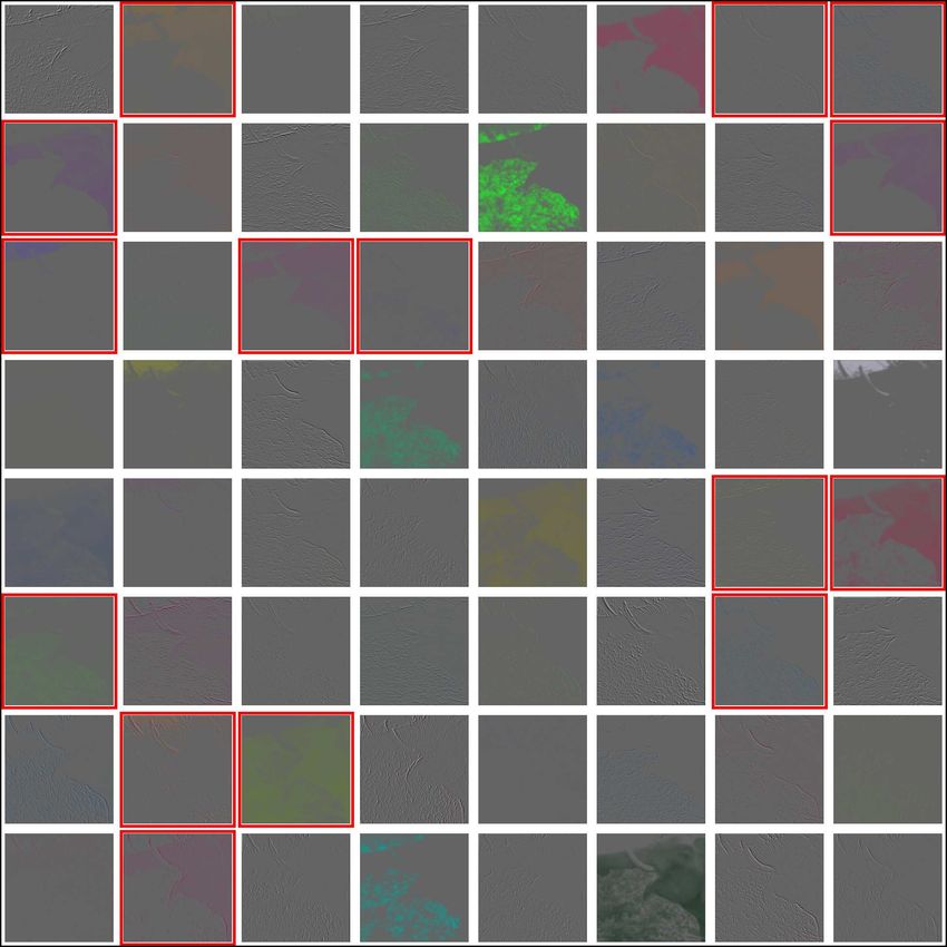
shown in Figure 4(b). After 30 epochs, the network is con-
vergent to adaptively obtain the salient filters and their masks
by dynamic updating. In Figure 4(c), several number of fil-
ters, masks and output feature maps are different with the
ones after the first updating, which indicates that the saliency
of filters were mistakenly judged in the beginning, but were
successfully updated during the dynamic updating.
(a) Epoch 0
5 Conclusion
This work presents a global dynamic pruning (GDP) scheme
to prune redundant filters for CNN acceleration. We employ
a global discriminative function based on prior knowledge of
each filter to globally prune the unsalient filters across all lay-
ers. To decrease accuracy loss caused by incorrect globally
pruning, we dynamically update the filter saliency all over
the pruned sparse network. Specially, we further handle the
corresponding non-convex optimization problem of the pro-
posed GDP, which is effectively solved via stochastic gradient
descent with greedy alternative updating. In experiments, the
(b) Epoch 1
proposed GDP achieves superior performance to accelerate
various cutting-edge CNNs on ILSVRC-12, comparing to the
state-of-the-art filter pruning methods.
Acknowledgments
This work is supported by the National Key R&D Pro-
gram (No.2017YFC0113000, and No.2016YFB1001503),
the Natural Science Foundation of China (No.U1705262,
No.61772443, No.61402388 and No.61572410), the Post
(c) Epoch 30 Doctoral Innovative Talent Support Program under Grant
BX201600094, the China Post-Doctoral Science Foundation
Figure 4: Dynamically update filters, masks and output feature maps under Grant 2017M612134, Scientific Research Project of
on the first layer of VGG-16. Left: filters and masks, Right: output
feature maps. In the left column, each rectangle contains filter and
National Language Committee of China (Grant No. YB135-
mask, in which the black one indicates the mask is unchanged, and 49), and Natural Science Foundation of Fujian Province,
the red one presents the filter and mask are updated. In addition, the China (No. 2017J01125 and No. 2018J01106).
mask is a smaller rectangle, in which indicates the corresponding
filter is salient, and is unsalient. In the right column, the feature References
maps changed correspondingly are shown in the red boxes.
[Abadi et al., 2016] Martı́n Abadi, Ashish Agarwal, Paul
Barham, Eugene Brevdo, Zhifeng Chen, Craig Citro,
a higher CPU and GPU speedup (5,012ms CPU and 242ms Greg S Corrado, Andy Davis, Jeffrey Dean, Matthieu
GPU online inference in GDP vs. 5,253ms CPU and 246ms Devin, et al. Tensorflow: Large-scale machine learn-
GPU online inference in CP). To explain, dynamic updating ing on heterogeneous distributed systems. arXiv preprint
in GDP significantly improves the discriminability and gen- arXiv:1603.04467, 2016.
eralization of the pruned network. [Anwar et al., 2015] Sajid Anwar, Kyuyeon Hwang, and
Wonyong Sung. Structured pruning of deep convolutional
4.3 Visualization of Dynamic Updating neural networks. arXiv preprint arXiv:1512.08571, 2015.
Quantitatively, we have testified the effectiveness of dynamic [Courbariaux and Bengio, 2016] M. Courbariaux and
updating in our global pruning scheme. To show the pro- Y. Bengio. Binarynet: Training deep neural networks
cess of dynamic updating, we visualize filters, masks and out- with weights and activations constrained to+ 1 or-1. arXiv
put feature maps of the first convolutional layer for VGG-16 preprint arXiv:1602.02830, 2016.
by using the proposed GDP method and setting β to be 0.5,
as presented in Figure 4. Before pruning the filters (i.e., the [Courbariaux et al., 2015] M. Courbariaux, Y. Bengio, and
masks all equal to 1), low-level features (e.g., edge, color and J. David. Binaryconnect: Training deep neural networks
corner detectors of various directions) can be found among with binary weights during propagations. In NIPS, 2015.
the listed filters and output feature maps, as shown in Fig- [Denton et al., 2014] Emily L Denton, Wojciech Zaremba,
ure 4(a). After the first-round mask updating, the network is Joan Bruna, Yann LeCun, and Rob Fergus. Exploiting
pruned temporarily by selecting the salient filters based on linear structure within convolutional networks for efficient
TE, and then is updated to adapt to the pruned network, as evaluation. In NIPS, pages 1269–1277, 2014.
2431Proceedings of the Twenty-Seventh International Joint Conference on Artificial Intelligence (IJCAI-18)
[Girshick et al., 2014] Ross Girshick, Jeff Donahue, Trevor Speeding-up convolutional neural networks using fine-
Darrell, and Jitendra Malik. Rich feature hierarchies for tuned cp-decomposition. arXiv preprint arXiv:1412.6553,
accurate object detection and semantic segmentation. In 2014.
CVPR, pages 580–587, 2014. [LeCun et al., 1989] Yann LeCun, John S Denker, Sara A
[Gong et al., 2014] Yunchao Gong, Liu Liu, Ming Yang, Solla, Richard E Howard, and Lawrence D Jackel. Op-
and Lubomir Bourdev. Compressing deep convolu- timal brain damage. In NIPS, 1989.
tional networks using vector quantization. arXiv preprint [Li et al., 2016] Hao Li, Asim Kadav, Igor Durdanovic,
arXiv:1412.6115, 2014. Hanan Samet, and Hans Peter Graf. Pruning filters for ef-
[Guo et al., 2016] Yiwen Guo, Anbang Yao, and Yurong ficient convnets. arXiv preprint arXiv:1608.08710, 2016.
Chen. Dynamic network surgery for efficient dnns. In [Lin et al., 2016] Shaohui Lin, Rongrong Ji, Xiaowei Guo,
NIPS, pages 1379–1387, 2016. and Xuelong Li. Towards convolutional neural networks
[Han et al., 2015a] Song Han, Huizi Mao, and William J compression via global error reconstruction. In IJCAI,
Dally. Deep compression: Compressing deep neural net- pages 1573–1759, 2016.
work with pruning, trained quantization and huffman cod- [Lin et al., 2017] Shaohui Lin, Rongrong Ji, Chao Chen, and
ing. CoRR, abs/1510.00149, 2, 2015. Feiyue Huang. Espace: Accelerating convolutional neural
[Han et al., 2015b] Song Han, Jeff Pool, John Tran, and networks via eliminating spatial & channel redundancy. In
William Dally. Learning both weights and connections for AAAI, pages 1424–1430, 2017.
efficient neural network. In NIPS, pages 1135–1143, 2015. [Liu et al., 2015] Baoyuan Liu, Min Wang, Hassan Foroosh,
[Han et al., 2016] Song Han, Xingyu Liu, Huizi Mao, Jing Marshall Tappen, and Marianna Pensky. Sparse convolu-
tional neural networks. In CVPR, pages 806–814, 2015.
Pu, Ardavan Pedram, Mark A Horowitz, and William J
Dally. Eie: efficient inference engine on compressed deep [Long et al., 2015] Jonathan Long, Evan Shelhamer, and
neural network. In ISCA, 2016. Trevor Darrell. Fully convolutional networks for seman-
tic segmentation. In CVPR, pages 3431–3440, 2015.
[Hassibi and Stork, 1993] Babak Hassibi and David G Stork.
Second order derivatives for network pruning: Optimal [Luo et al., 2017] Jianhao Luo, Jianxin Wu, and Weiyao Lin.
brain surgeon. In NIPS, 1993. Thinet: A filter level pruning method for deep neural net-
work compression. In ICCV, 2017.
[He et al., 2016] Kaiming He, Xiangyu Zhang, Shaoqing
[Molchanov et al., 2017] Pavlo Molchanov, Stephen Tyree,
Ren, and Jian Sun. Deep residual learning for image recog-
nition. In CVPR, pages 770–778, 2016. Tero Karras, Timo Aila, and Jan Kautz. Pruning convo-
lutional neural networks for resource efficient inference.
[Hu et al., 2016] Hengyuan Hu, Rui Peng, Yu-Wing Tai, and In ICLR, 2017.
Chi-Keung Tang. Network trimming: A data-driven neu- [Park et al., 2017] Jongsoo Park, Sheng Li, Wei Wen, Ping
ron pruning approach towards efficient deep architectures.
Tak Peter Tang, Hai Li, Yiran Chen, and Pradeep Dubey.
arXiv preprint arXiv:1607.03250, 2016.
Faster cnns with direct sparse convolutions and guided
[Jaderberg et al., 2014] Max Jaderberg, Andrea Vedaldi, and pruning. In IJCAI, 2017.
Andrew Zisserman. Speeding up convolutional neu- [Rastegari et al., 2016] M. Rastegari, V. Ordonez, J. Red-
ral networks with low rank expansions. arXiv preprint mon, and A. Farhadi. Xnor-net: Imagenet classification
arXiv:1405.3866, 2014. using binary convolutional neural networks. arXiv preprint
[Jia et al., 2014] Yangqing Jia, Evan Shelhamer, Jeff Don- arXiv:1603.05279, 2016.
ahue, Sergey Karayev, Jonathan Long, Ross Girshick, Ser- [Russakovsky et al., 2015] Olga Russakovsky, Jia Deng,
gio Guadarrama, and Trevor Darrell. Caffe: Convolutional Hao Su, Jonathan Krause, Sanjeev Satheesh, Sean Ma,
architecture for fast feature embedding. In ACM MM, Zhiheng Huang, Andrej Karpathy, Aditya Khosla, Michael
pages 675–678. ACM, 2014. Bernstein, Alexander C. Berg, and Li Fei-Fei. Ima-
[Kim et al., 2015] Yong-Deok Kim, Eunhyeok Park, geNet Large Scale Visual Recognition Challenge. Inter-
Sungjoo Yoo, Taelim Choi, Lu Yang, and Dongjun Shin. national Journal of Computer Vision (IJCV), 115(3):211–
Compression of deep convolutional neural networks for 252, 2015.
fast and low power mobile applications. arXiv preprint [Simonyan and Zisserman, 2014] Karen Simonyan and An-
arXiv:1511.06530, 2015. drew Zisserman. Very deep convolutional networks
[Krizhevsky et al., 2012] Alex Krizhevsky, Ilya Sutskever, for large-scale image recognition. arXiv preprint
and Geoffrey E Hinton. Imagenet classification with deep arXiv:1409.1556, 2014.
convolutional neural networks. In NIPS, 2012. [Wen et al., 2016] Wei Wen, Chunpeng Wu, Yandan Wang,
[Lebedev and Lempitsky, 2016] Vadim Lebedev and Victor Yiran Chen, and Hai Li. Learning structured sparsity in
Lempitsky. Fast convnets using group-wise brain damage. deep neural networks. In NIPS, 2016.
In CVPR, pages 2554–2564, 2016. [Wu et al., 2016] Jiaxiang Wu, Cong Leng, Yuhang Wang,
[Lebedev et al., 2014] Vadim Lebedev, Yaroslav Ganin, Qinghao Hu, and Jian Cheng. Quantized convolutional
Maksim Rakhuba, Ivan Oseledets, and Victor Lempitsky. neural networks for mobile devices. In CVPR, 2016.
2432You can also read