Hallucinating Saliency Maps for Fine-Grained Image Classification for Limited Data Domains
←
→
Page content transcription
If your browser does not render page correctly, please read the page content below
Hallucinating Saliency Maps for Fine-Grained Image Classification for
                                                                    Limited Data Domains

                                                Carola Figueroa-Flores1,2 , Bogdan Raducanu 1 , David Berga 1 and Joost van de Weijer 1
                                                                                          1 Computer Vision Center

                                                                                        Edifici “O” - Campus UAB
                                                                                    8193 Bellaterra (Barcelona), Spain
                                                                       2 Department of Computer Science and Information Technology

                                                                                       Universidad del Bı́o Bı́o, Chile
                                                                    {cafigueroa, bogdan, dberga, joost}@cvc.uab.es, cfiguerf@ubiobio.cl
arXiv:2007.12562v2 [cs.CV] 30 Oct 2020

                                         Keywords:      Fine-grained image classification, Saliency detection, Convolutional neural networks

                                         Abstract:      It has been shown that saliency maps can be used to improve the performance of object recognition systems,
                                                        especially on datasets that have only limited training data. However, a drawback of such an approach is that it
                                                        requires a pre-trained saliency network. In the current paper, we propose an approach which does not require
                                                        explicit saliency maps to improve image classification, but they are learned implicitely, during the training
                                                        of an end-to-end image classification task. We show that our approach obtains similar results as the case
                                                        when the saliency maps are provided explicitely. We validate our method on several datasets for fine-grained
                                                        classification tasks (Flowers, Birds and Cars), and show that especially for domains with limited data the
                                                        proposed method significantly improves the results.

                                         1    INTRODUCTION                                                fication of semantic parts using either explicit annota-
                                                                                                          tion [Zhang et al., 2014, Lin et al., 2015, Zhang et al.,
                                                                                                          2016a, Ding et al., 2019, Du et al., 2020] or weak la-
                                             Fine-grained image recognition has as objec-
                                                                                                          beling [Zheng et al., 2017,Fu et al., 2017,Wang et al.,
                                         tive to recognize many subcategories of a super-
                                                                                                          2020]. The main disadvantage of these approaches
                                         category. Examples of well-known fine-grained
                                                                                                          was that they required two different ’pipelines’, for
                                         datasets are Flowers [Nilsback and Zisserman, 2008],
                                                                                                          detection and classification, which makes the joint op-
                                         Cars [Krause et al., 2013] and Birds [Welinder et al.,
                                                                                                          timization of the two subsystems more complicated.
                                         2010]. The challenge of fine-grained image recog-
                                                                                                          Therefore, more recent approaches are proposing end-
                                         nition is that the differences between classes are of-
                                                                                                          to-end strategies with the focus on improving the fea-
                                         ten very subtle, and only the detection of small highly
                                                                                                          ture representation from intermediate layers in a CNN
                                         localized features will correctly lead to the recogni-
                                                                                                          through higher order statistics modeling [Cai et al.,
                                         tion of the specific bird or flower species. An ad-
                                                                                                          2017, Wang et al., 2018a].
                                         ditional challenge of fine-grained image recognition
                                         is the difficulty of data collection. The labelling of               One recent approach which obtained good fine-
                                         these datasets requires experts and subcategories can            grained recognition results, especially with only few
                                         be very rare which further complicates the collection            labeled data is proposed in [Flores et al., 2019]. The
                                         of data. Therefore, the ability to train high-quality im-        main idea is that a saliency image can be used to
                                         age classification systems from few data is an impor-            modulate the recognition branch of a fine-grained
                                         tant research topic in fine-grained object recognition.          recognition network. We will refer to this technique
                                             Most of the state-of-the-art general object classi-          as saliency-modulated image classification (SMIC).
                                         fication approaches [Wang et al., 2017, Krizhevsky               This is especially beneficial when only few labeled
                                         et al., 2012] have difficulties in the fine-grained recog-       data is available. The gradients which are backprop-
                                         nition task, which is more challenging due to the fact           agated are concentrated on the regions which have
                                         that basic-level categories (e.g. different bird species         high saliency. This prevents backpropagation of gra-
                                         or flowers) share similar shape and visual appearance.           dients of uninformative background parts of the im-
                                         Early works have focused on localization and classi-             age which could lead to overfitting to irrelevant de-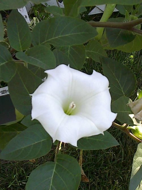
Step I: Training on Imagenet                        Step II: Finetuning on a fine-grained dataset
                                                                                        Approach A                               Approach B

            Saliency            RGB                               Saliency             RGB                        Saliency    RGB
            Branch             Branch                             Branch              Branch                      Branch     Branch

                                   Initialize weights:                                         Finetuning:

                                   Random initialization                                       Finetuned layers

                                   Pretrained network                                          Frozen layers

Figure 1: Overview of our method. We process an RGB input image through two branches: one branch extracts the RGB
features and the other one is used to learn saliency maps. The resulting features are merged via a modulation layer, which
continues with a few more convolutional layers and a classification layer. The network is trained in two steps.

tails. A major drawback of this approach is that it                                  tion using a subset from ImageNet validation dataset.
requires an explicit saliency algorithm which needs to                               During this process, the saliency branch will learn
be trained on a saliency dataset.                                                    to identify which regions are more discriminative.
    In order to overcome the lack of sufficient data for                             In a second phase, we initialize the weights of the
a given modality, a common strategy is to introduce                                  saliency branch with these pre-trained weights. We
a ’hallucination’ mechanism which emulates the ef-                                   then train the system end-to-end on the fine-grained
fect of genuine data. For instance, in [Hoffman et al.,                              dataset using only the RGB images. Results show that
2016], they use this ’hallucination’ strategy for RGB-                               the saliency branch improves fine-grained recognition
D object detection. A hallucination network is trained                               significantly, especially for domains with few training
to learn complementary RGB image representation                                      images.
which is taught to mimic convolutional mid-level fea-                                    We briefly summarize below our main contribu-
tures from a depth network. At test time, images are                                 tions:
processed jointly through the RGB and hallucination
networks, demonstrating an improvement in detection                                    • we propose an approach which hallucinates
performance. This strategy has been adopted also for                                     saliency maps that are fused together with the
the case of few-shot learning [Hariharan and Girshick,                                   RGB modality via a modulation process,
2017, Wang et al., 2018b, Zhang et al., 2019]. In this
case, the hallucination network has been used to pro-                                  • our method does not require any saliency maps
duce additional training sample used to train jointly                                    for training (like in these works [Murabito et al.,
with the original network (also called a neta-learner).                                  2018, Flores et al., 2019]) but instead is trained
                                                                                         indirectly in an end-to-end fashion by training the
    In this paper, we address the major drawback of                                      network for image classification,
SMIC, by implementing a hallucination mechanism
in order to remove the requirement for providing                                       • our method improves classification accuracy on
saliency images for training obtained using one of the                                   three fine-grained datasets, especially for domains
existing algorithms [Bylinskii et al., ]. In other words,                                with limited data.
we show that the explicit saliency branch which re-
quires training on a saliency image dataset, can be re-                                  The paper is organized as follows. Section II is
placed with a branch which is trained end-to-end for                                 devoted to review the related work in fine-grained im-
the task of image classification (for which no saliency                              age classification and saliency estimation. Section III
dataset is required). We replace the saliency image                                  presents our approach. We report our experimental
with the input RGB image (see Figure 1). We then                                     results in Section IV. Finally, Section V contains our
pre-train this network for the task of image classifica-                             conclusions.
2     RELATED WORK                                         (using a random jigsaw patch generator) and after-
                                                           wards fuse them together. Some other works intro-
                                                           duce an attention mechanism. For instance, [Zheng
2.1    Fine-grained image classification                   et al., 2017] propose a novel part learning approach by
                                                           a multi-attention convolutional neural network (MA-
A first group of approaches on fine-grained recogni-       CNN) without bounding box/part annotations. MA-
tion operate on a two-stage pipeline: first detecting      CNN jointly learns part proposals (defined as multi-
some object parts and then categorizing the objects        ple attention areas with strong discrimination ability)
using this information.                                    and the feature representations on each part. Simi-
     The work of [Huang et al., 2016] first localizes      lar approaches have been in reported in [Sun et al.,
a set of part keypoints, and then simultaneously pro-      2018, Luo et al., 2019]. In [Ding et al., 2019], they
cesses part and object information to obtain highly        propose a network which learns sparse attention from
descriptive representations. Mask-CNN [Wei et al.,         class peak responses (which usually corresponds to
2018] also aggregates descriptors for parts and objects    informative object parts) and implements spatial and
simultaneously, but using pixel-level masks instead of     semantic sampling. Finally, in [Ji et al., 2020], the au-
keypoints. The main drawback of these models is the        thors present an attention convolutional binary neural
need of human annotation for the semantic parts in         tree in a weakly-supervised approach. Different root-
terms of keypoints or bounding boxes. To partially         to-leaf paths in the tree network focus on different
alleviate this tedious task of annotation, [Xiao et al.,   discriminative regions using the attention transformer
2015] propose an weakly-supervised approach based          inserted into the convolutional operations along edges
on the combination of three types of attention in or-      of the tree. The final decision is produced as the sum-
der to guide the search for object parts in terms of       mation of the predictions from the leaf nodes.
’what’ and ’where’. A further improvement has been             In another direction, some end-to-end frameworks
reported in [Zhang et al., 2016b], where the authors       aim to enhance the intermediate representation learn-
propose and approach free of any object / part anno-       ing capability of a CNN by encoding higher-order
tation. Their method explores a unified framework          statistics. For instance in [Gao et al., 2016] they cap-
based on two steps of deep filter response picking.        ture the second-order information by taking the outer-
On the other hand, [Wang et al., 2020] propose an          product over the network output and itself. Other
end-to-end discriminative feature-oriented Gaussian        approaches focuses on reducing the high feature di-
Mixture Model (DF-GMM) to learn low-rank feature           mensionality [Kong and Fowlkes, 2017] or extract-
maps which alleviates the discriminative region diffu-     ing higher order information with kernelized mod-
sion problem in high-level feature maps and thus find      ules [Cai et al., 2017]. In [Wang et al., 2018a], they
better fine-grained details.                               learn a bank of convolutional filters that capture class-
     A second group of approaches merges these two         specific discriminative patches without extra part or
stages into an end-to-end learning framework which         bounding box annotations. The advantage of this ap-
optimize simultaneously both part localization and         proach is that the network focuses on classification
fine-grained classification. This is achieved by first     only and avoids the trade-off between recognition and
finding the corresponding parts and then comparing         localization.
their appearance [Wang et al., 2018a]. In [Xie et al.,         Regardless, most fine-grained approaches use the
2017], their framework first performs unsupervised         object ground-truth bounding box at test time, achiev-
part candidates discovery and global object discovery      ing a significantly lower performance when this in-
which are subsequently fed into a two-stream CNN in        formation is not available. Moreover, automatically
order to model jointly both the local and global fea-      discovering discriminative parts might require large
tures. In [Chen et al., 2019], they propose an approach    amounts of training images. Our approach is more
based on ’Destruction and Construction Learning’           general, as it only requires image level annotations
whose purpose is to force the network to understand        at training time and could easily generalize to other
ç¡‘the semantics of each region. For destruction, a re-   recognition tasks.
gion confusion mechanism (RCM) forces the classifi-
cation network to learn from discriminative regions.
For construction, the region alignment network re-         2.2    Saliency estimation
stores the original region layout by modeling the se-
mantic correlation among regions. A similar idea           Initial efforts in modelling saliency involved multi-
has been pursued in [Du et al., 2020], where they          scale representations of color, orientation and inten-
propose a progressive training strategy to encourage       sity contrast. These were often biologically inspired
the network to learn features at different granularities   such as the well-known work by Itti et al. [Itti et al.,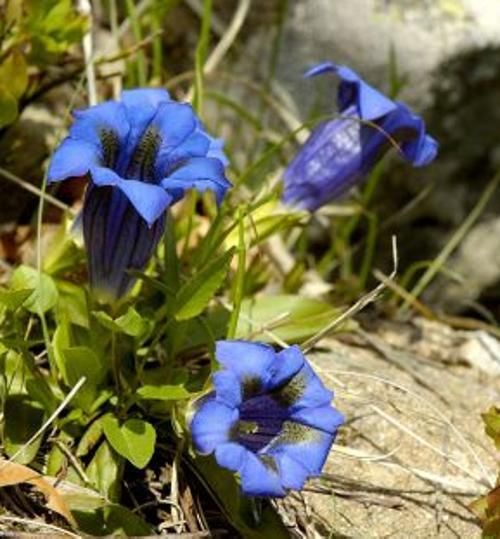
1998]. From that model, a myriad of models were             generate the saliency map from the same RGB im-
based on handcrafting these features in order to obtain     age. Both branches are combined using a modula-
an accurate saliency map [Borji and Itti, 2013, Bylin-      tion layer (represented by the × symbol) and are then
skii et al., 2015], either maximizing [Bruce and Tsot-      processed by several shared layers of the joint branch
sos, 2005] or learning statistics of natural images         which finally ends up with a classification layer. The
[Torralba et al., 2006, Harel et al., 2007]. Saliency       RGB branch followed by the joint branch resembles
research was propelled further by the availability of       a standard image classification network. The novelty
large data sets which enabled the use machine learn-        of our architecture is the introduction of the saliency
ing algorithms [Borji, 2018], mainly pretrained on ex-      branch, which transforms the generated saliency im-
isting human fixation data.                                 age into a modulation image. This modulation image
    The question of whether saliency is important for       is used to modulate the characteristics of the RGB
object recognition and object tracking has been raised      branch, putting more emphasis on those characteris-
in [Han and Vasconcelos, 2010]. Latest methods              tics that are considered important for the fine-grained
[Borji, 2018] take advantage of end-to-end convolu-         recognition task. In the following sections we pro-
tional architectures by finetuning over fixation predic-    vide the details of the network architecture, the op-
tion [Kümmerer et al., 2016, Pan et al., 2017, Cornia      eration of the modulation layer, and finally, how our
et al., 2018]. But the main goal of these works was         saliency map is generated. We explain our model us-
to estimate a saliency map, not how saliency could          ing AlexNet [Krizhevsky et al., 2012] as the base clas-
contribute to object recognition. In this paper instead,    sification network, but the theory could be extended
we propose an approach which does not require ex-           to other convolutional neural network architectures.
plicit saliency maps to improve image classification,       For instance, in the experimental results section, we
but they are learned implicitly, during the training of     also consider the ResNet-152 architecture [He et al.,
an end-to-end image classification task. We show that       2016].
our approach obtains similar results as the case when
the saliency maps are provided explicitely.                 3.2    Hallucination of saliency maps from
                                                                   RGB images

3     PROPOSED METHOD                                       The function of the visual attention maps is to fo-
                                                            cus on the location of the characteristics necessary to
    Several works have shown that having the saliency       identify the target classes, ignoring anything else that
map of an image can be helpful for object recognition       may be irrelevant to the classification task. There-
and fine-grained recognition in particular [Murabito        fore, given an input RGB image, our saliency branch
et al., 2018, Flores et al., 2019]. The idea is twofold:    should be able to produce a map of the most salient
the saliency map can help focus the attention on the        image locations useful for classification purposes.
relevant parts of the image to improve the recogni-             To achieve that, we apply a CNN-based saliency
tion, and it can help guide the training by focusing        detector consisting of four convolutional layers
the backpropagation to the relevant image regions. In       (based on the AlexNet architecture)1 . The output
[Flores et al., 2019], the authors show that saliency-      from the last convolutional layer, i.e. one with 384
modulated image classification (SMIC) is especially         dimensional feature maps with a spatial resolution of
efficient for training on datasets with few labeled data.   13 × 13 (for a 227 × 227 RGB input image), is fur-
The main drawback of these methods is that they re-         ther processed using a 1 × 1 convolution and then a
quire a trained saliency method. Here we show that          function of activation ReLU. This is to calculate the
this restriction can be removed and that we can hal-        saliency score for each ”pixel” in the feature maps of
lucinate the saliency image from the RGB image. By          the previous layer, and to produce a single channel
training the network for image classification on the        map. Finally, to generate the input for the subsequent
imageNet dataset we can obtain the saliency branch          classification network, the 13 × 13 saliency maps are
without human groundtruth images.                           upsampled to 27 × 27 (which is the default input size
                                                            of the next classification module) through bilinear in-
3.1    Overview of the Method                               terpolation. We justify the size of the output maps by
                                                            claiming that saliency is a primitive mechanism, used
                                                            by humans to direct attention to objects of interest,
The overview of our proposed network architecture
                                                            which is evoked by coarse visual stimuli. Therefore,
is illustrated in Figure 1. Our network consists of
two branches: one to extract the features from an              1 Wevary the number of convolutional layers in the ex-
RGB image, and the other one (saliency branch) to           perimental section and found four to be optimal.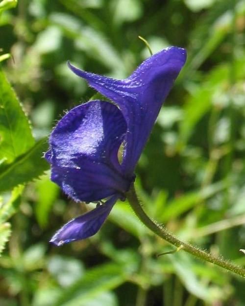
our experiments (see section IV) show that 13 × 13
feature maps can encode the information needed to 92
detect salient areas and drive a classifier with them. 91
3.3 Fusion of RGB and Saliency 90
Branches 89
Consider an input image I(x, y, z), where z = {1, 2, 3} 88
indicate the three color channels of the image. Also
1
2
3
4
e
lin
consider a saliency map s(x, y). In Flores et al. [Flo-
-
-
-
-
nv
nv
nv
nv
se
Co
Co
Co
Co
Ba
res et al., 2019], a network h (I, s) was trained which
performed image classification based on the input im- Figure 2: Graph shows the classification accuracy on Flow-
age I and the saliency map s. Here, we replace the ers for various number of layers in the saliency branch. Best
results are obtained with four convolutional layers. Baseline
saliency map (which was generated by a saliency al-
refers to the method without saliency branch.
gorithm) by a hallucinated saliency map h (I, s̊ (I)).
The hallucinated saliency map s̊ is trained end-to-end
and estimated from the same input image I without 92
the need of any ground truth saliency data.
The combination of the hallucinated saliency map 91
s̊ , which is the output of the saliency branch, and the
90
RGB branch is done with modulation. Consider the
output of the ith layer of the network, l i , with dimen- 89
sion wi × hi × zi . Then we define the modulation as
88
lˆi (x, y, z) = l i (x, y, z) · s̊ (x, y) , (1)
resulting in the saliency-modulated layer lˆi . Note that
l-2
l-2
3
4
e
in
v-
v-
oo
oo
l
on
on
se
eP
rP
rC
rC
Ba
a single hallucinated saliency map is used to modulate
fte
or
fte
fte
f
A
Be
A
A
all i feature maps of l.ˆ
In addition to the formula in Eq. (1) we also intro- Figure 3: Graph shows the classification accuracy on Flow-
ers. Various points for fusing the saliency and RGB branch
duce a skip connection from the RGB branch to the
are evaluated. Best results are obtained when fusion is
beginning of the joint branch, defined as placed before the pool-2 layer. Baseline refers to the
lˆi (x, y, z) = l i (x, y, z) · (s̊ (x, y) + 1) . (2) method without saliency branch.
This skip connection is depicted in Figure 1 (+ sym- 3.4 Training on Imagenet and
bol). It prevents the modulation layer from com-
pletely ignoring the features from the RGB branch.
fine-tuning on a target dataset
This is inspired by this work [Flores et al., 2019] that
found this approach beneficial when using attention As can be seen in Figure 1, the training of our ap-
for network compression. proach is divided into two steps: first, training on Im-
We train our architecture in an end-to-end manner. agenet and second, fine-tuning on a target dataset.
The backpropagated gradient for the modulation layer Step 1: Training of saliency branch on Imagenet.
into the image classification branch is equal defined As explained above, the aim of the saliency branch
as: is to hallucinate (generate) a saliency map directly
∂L ∂L from an RGB input image. This network is con-
= · (s̊ (x, y) + 1) , (3)
∂l i ∂lˆi structed by initializing the RGB branch with pre-
where L is the loss function of the network. We can trained weights from Imagenet. The weights of the
see that the saliency map modulates both the forward saliency branch are initialized randomly using the
pass (see Eq. (2)) as well as the backward pass in the Xavier method (see Figure 1, left image). The net-
same manner; in both cases putting more weight on work is then trained selectively, using the ImageNet
the features that are on locations with high saliency, validation set: we allow to train only the layers corre-
and putting less weight on the irrelevant features. We sponding to the saliency branch (depicted by the sur-
show in the experiments that this helps the network rounding dotted line) and freeze all the remaining lay-
train more efficiently, also on datasets with only few ers (depicted through the continuous line boxes).
labeled samples. The modulation prevents the net- Step 2: Fine-tuning on a target dataset. In this step,
work from overfitting to the background. we initialize the RGB branch with the weights pre-
#train images                   1      2      3       5       10     15      20      25     30      K      AVG
           Baseline-RGB                  31.8   45.8    53.1    63.6    72.4   76.9    81.2    85.1   87.2    87.8    68.3
 Flowers

           Baseline-RGB + scratch SAL    34.3   48.9    54.3    65.9    73.1   77.4    82.3    85.9   88.9    89.1    70.0
           SMIC [Flores et al., 2019]∗   37.6   51.9    57.1    68.5    75.2   79.7    84.9    88.2   91.2    92.3    72.7
           Approach A                    36.9   51.3    56.9    67.8    74.9   78.4    82.9    88.1   90.9    92.0    72.0
           Approach B                    37.3   51.7    57.2    68.7    75.6   78.7    83.8    88.4   91.7    92.5    72.6
           Baseline-RGB                   4.1    7.8    11.7    17.3    25.5   31.1    38.5    42.2   47.2    60.0    28.5
           Baseline-RGB + scratch SAL     5.9   10.7    14.4    19.1    27.4   32.9    38.5    44.0   48.7    61.5    30.3
           SMIC [Flores et al., 2019]∗    9.3   14.0    18.0    22.8    30.0   34.7    40.4    46.0   50.0    61.4    32.7
 Cars

           Approach A                     9.3   14.3    17.4    22.3    28.4   35.3    39.7    45.7   50.1    61.9    32.4
           Approach B                     9.8   15.1    18.4    22.9    28.8   35.1    39.9    45.8   49.7    62.9    32.8
           Baseline-RGB                   9.1   13.6    19.4    27.7    37.8   44.3    48.0    50.0   54.2    57.0    34.8
           Baseline-RGB + scratch SAL    10.4   14.9    20.3    28.3    38.6   43.9    46.9    48.4   50.7    55.7    35.8
           SMIC [Flores et al., 2019]∗
 Birds

                                         13.1   18.9    22.2    30.2    38.7   44.3    48.0    50.0   54.2    57.0    37.7
           Approach A                    11.8   18.3    22.1    29.3    39.1   44.4    47.8    49.7   53.1    56.5    37.2
           Approach B                    12.9   18.7    22.7    29.7    39.4   44.1    48.2    49.9   53.9    57.7    37.7
Table 1: Classification accuracy for Flowers, Cars, and Birds dataset (results are the average over three runs), using AlexNet
as base network. Results are provided for varying number of training images, from 1 until 30; K refers to using the number
of training images used in the official dataset split. The rightmost column shows the average. The ∗ indicates that the method
requires an explicit saliency method. Our method (Approach B) obtains similar results as SMIC but without the need of a
pretrained saliency network trained on a saliency dataset.

trained from Imagenet and the saliency branch with                  • Birds: CUB200 has 11.788 images of 200 differ-
the corresponding pre-trained weights from Step 1.                    ent bird species [Welinder et al., 2010].
The weights of the top classification layer are initial-            • Cars: the CARS-196 dataset in [Krause et al.,
ized randomly, using the Xavier method. Then, this                    2013] contains 16,185 images of 196 car classes.
network is then further fine-tuned on a target dataset,
selectively. We distinguish two cases:                            Network architectures.                We evaluate our
                                                                  approach using two network architectures:
 • Approach A: We freeze the layers of the saliency               Alexnet [Krizhevsky et al., 2012] and Resnet-
   branch and we allow all the other layers layers in             152 [He et al., 2016]. In both cases, the weights were
   the network to be trained. This process is depicted            pretrained on Imagenet and then finetuned on each
   by the continuous line surrounding the saliency                of the datasets mentioned above. The networks were
   branch and the dotted line for the rest (see the Fig-          trained for 70 epochs with a learning rate of 0.0001
   ure 1, middle image).                                          and a weight decay of 0.005. The top classification
 • Approach B: We allow all layers to be trained.                 layer was initialized from scratch using Xavier
   Since we consider training on datasets with only               method [Glorot and Bengio, 2010].
   few labels this could results in overfitting, since it         Evaluation protocol. To validate our approach,
   requires all the weights of the saliency branch to             we follow the same protocol as in [Flores et al.,
   be learned (see the Figure 1, right image) .                   2019]. For the image classification task, we train
In the experiments we evaluate both approaches to                 each model with subsets of k training images for
training the network.                                             k ∈ {1, 2, 3, 5, 10, 15, 20, 25, 30, K}, where k is the to-
                                                                  tal number of training images for the class. We keep 5
                                                                  images per class for validation and 5 images per class
                                                                  for test. We report the performance in terms of accu-
4          EXPERIMENTS                                            racy, i.e. percentage of correctly classified samples.
                                                                  We show the results as an average over three runs.
4.1         Experimental Setup
                                                                  4.2    Fine-grained Image Classification
Datasets. To evaluate our approach, we used three                        Results
standard datasets used for fine-grained image classifi-
cation:                                                           Optimal depth and fusion saliency branch: First
 • Flowers: Oxford Flower 102 dataset [Nilsback                   we evaluate the saliency branch with a varying num-
   and Zisserman, 2008] has 8.189 images divided                  ber of convolutional layers. The results are presented
   in 102 classes.                                                in Figure 2. We found that four convolutional layers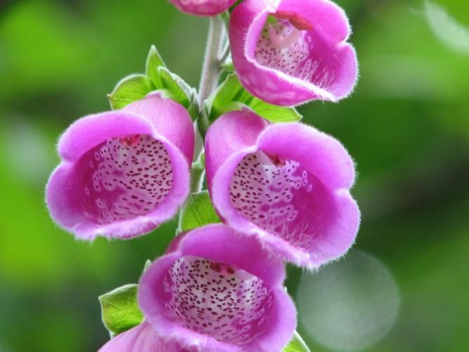
#train images                  1       2       3       5      10      15      20      25      30      K      AVG
           Baseline-RGB                  39.0    60.1    68.0    82.5   89.0    92.0    92.1    93.3    94.2    95.4    80.3
 Flowers

           Baseline-RGB + scratch SAL    40.1    63.8    69.7    83.9   89.7    91.9    92.9    93.8    95.1    97.1    81.8
           SMIC [Flores et al., 2019]∗   42.6    64.2    70.9    85.5   90.9    92.7    94.0    95.0    97.0    97.8    83.1
           Approach A                    42.4    64.5    70.7    85.2   90.3    92.4    93.3    94.3    96.5    97.9    82.8
           Approach B                    42.7    64.5    71.0    85.1   90.4    92.5    93.1    94.7    96.8    98.1    82.9
           Baseline-RGB                  30.9    45.8    53.1    62.7   70.9    73.9    79.9    88.7    89.2    90.7    68.6
           Baseline-RGB + scratch SAL    33.8    46.1    54.8    63.8   71.7    74.9    80.9    88.1    89.1    91.0    69.4
           SMIC [Flores et al., 2019]∗   34.7    47.9    55.2    64.9   72.1    75.8    82.1    90.0    91.1    92.4    70.6
 Cars

           Approach A                    34.1    47.0    56.3    64.7   71.9    75.3    81.7    89.0    90.8    91.7    70.2
           Approach B                    34.0    47.5    55.4    64.7   71.8    75.5    81.9    89.3    91.0    92.1    70.3
           Baseline-RGB                  24.9    35.3    44.1    53.3   63.8    71.8    75.7    79.3    82.9    83.7    61.5
           Baseline-RGB + scratch SAL    26.3    36.1    45.2    53.9   64.3    72.1    76.3    79.9    83.1    83.4    62.1
           SMIC [Flores et al., 2019]∗
 Birds

                                         28.1    37.9    46.8    55.2   65.3    73.1    77.0    82.9    84.4    86.1    63.7
           Approach A                    26.9    36.9    46.1    54.2   64.9    72.8    77.1    81.4    83.4    84.8    62.9
           Approach B                    27.1    37.0    46.2    54.9   65.4    72.8    77.1    81.3    83.8    85.1    63.1
Table 2: Classification accuracy for Flowers, Cars, and Birds dataset (results are the average over three runs), using ResNet152
as base network. Results are provided for varying number of training images, from 1 until 30; K refers to using the number
of training images used in the official dataset split. The rightmost column shows the average. The ∗ indicates that the method
requires an explicit saliency method. Our method (Approach B) obtains similar results as SMIC but without the need of a
pretrained saliency network trained on a saliency dataset.

led to a significant increase in performance. In addi-             the SMIC approach, where an additional algorithm is
tion, we look at the best RGB branch layer to perform              needed to generate the salience map. It is therefore
the fusion of the saliency branch and the RGB branch.              advantageous to also finetune the saliency branch on
The results are presented in Figure 3. It is found to be           the target data even when we only have a few labeled
optimal to fuse the two branches before the Pool-2                 images per class.
layer for AlexNet2 . Based on these experiments, we                    In Table 2, we show the same results but now for
use four convolutional layers in the saliency branch               ResNet152. One can see that the results improve sig-
and fuse before the second pool layer for the remain-              nificantly, especially for Cars results improve a lot.
der of the experiments and for all datasets.                       The same general conclusions can be drawn : Ap-
    Evaluation on scarce data domain: As de-                       proach B obtains better results than Approach A and
scribed in section III, we consider two alternative                the method obtains similar results as SMIC but with-
ways to train the saliency branch on the target dataset:           out the need of a pretrained saliency network.
keeping the saliency branch fixed (Approach A) or al-              Qualitative results: Table 3 shows some qualitative
lowing it to finetune (Approach B). In this section,               results for the case when the pretrained version of
we compare these two approaches with respect to                    our approach predicts the correct label, meanwhile the
the Baseline-RGB and Baseline-RGB + scratch SAL                    Baseline-RGB fails. Alternatively, in Table 4 depicts
(where Saliency branch is initialized from scratch                 the opposite case: the Baseline-RGB predicts the cor-
without pretraining on Imagenet). In addition, we                  rect label of the test images, meanwhile the pretrained
compare to the SMIC method of Flores et al. [Flo-                  version of our approach fails. In both cases, the
res et al., 2019] who also reports results for small               saliency images have been generated using our Ap-
training datasets. We do not compare to other fine-                proach B. A possible explanation for the failures in
grained methods here, because they do not report                   this latter case could be that the saliency images are
results when only considering few labeled images.                  not able to capture the relevant region of the image
The experiments are performed on Flowers, Cars and                 for fine-grained discrimination. Thus, the salience-
Birds datasets and can be seen in Table 1. The aver-               modulated layer focuses on the wrong features for the
age improvement of accuracy of our Approach A and                  task.
B with respect the Baseline-RGB is 3.7% and 4.3%,
respectively for the Flowers dataset; 3.9% and 4.3%,
respectively for the Cars dataset; and 2.4% and 2.9%,              CONCLUSIONS
respectively for the Birds dataset. Our Approach B
is especially advantageous when we compare it with
                                                                       In this work, we proposed a method to improve
      2 In
       a similar study, we found that for Resnet-152 the           fine-graned image classification by means of saliency
optimal fusion is after the forth residual block.                  maps. Our method does not require explicit saliency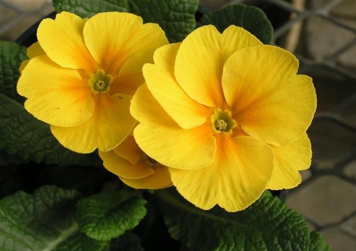
Table 3: Some success examples on Flowers: when the pre-
diction done by Baseline-RGB fails to infer the right label REFERENCES
for some test images, but the prediction by our approach
is correct. Example image contains image of the wrongly Borji, A. (2018). Saliency prediction in the deep learn-
predicted class. ing era: Successes, limitations, and future challenges.
.
Input Image Our Saliency Example Image
arXiv, arXiv:1810.03716.
Borji, A. and Itti, L. (2013). State-of-the-art in visual atten-
tion modeling. IEEE Transactions on Pattern Analysis
and Machine Intelligence, 35(1):185–207.
Bruce, N. D. B. and Tsotsos, J. K. (2005). Saliency based
Predicted (Baseline-RGB): StemlessGentian on information maximization. In Proceedings of the
Predicted (Our Approach B): Moonkshood 18th International Conference on Neural Information
Ground Truth: Moonkshood Processing Systems, NIPS’05, pages 155–162, Cam-
bridge, MA, USA. MIT Press.
Bylinskii, Z., DeGennaro, E., Rajalingham, R., Ruda, H.,
Zhang, J., and Tsotsos, J. (2015). Towards the quan-
Predicted (Baseline-RGB): Watercress
titative evaluation of visual attention models. Vision
Predicted (Our Approach B): Primula
Research, 116:258–268.
Ground Truth: Primula Bylinskii, Z., Judd, T., Borji, A., Itti, L., Durand, F.,
Oliva, A., and Torralba, A. Mit saliency benchmark.
http://saliency.mit.edu/.
Cai, S., Zuo, W., and Zhang, L. (2017). Higher-order in-
tegration of hierarchical convolutional activations for
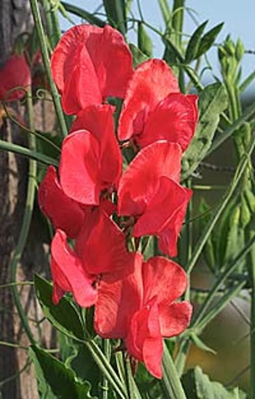
Predicted (Baseline-RGB): Sweet Pea fine-grained visual categorization. In Proc. of ICCV,
Predicted (Our Approach B): Snap dragon pages 511–520.
Ground Truth: Snap dragon
Chen, Y., Bai, Y., Zhang, W., and Mei, T. (2019). Destruc-
tion and construction learning for fine-grained image
Table 4: Some failure examples on Flowers: when the pre-
recognition. In Proc. of CVPR, pages 5157–5166.
diction done by our method fails to infer the right label for
some test images, but the prediction by Baseline-RGB is Cornia, M., Baraldi, L., Serra, G., and Cucchiara, R. (2018).
correct. Example image contains image of the wrongly pre- Predicting Human Eye Fixations via an LSTM-based
dicted class. Saliency Attentive Model. IEEE Transactions on Im-
. age Processing, 27(10):5142–5154.
Input Image Our Saliency Example Image
Ding, Y., Zhou, Y., Zhu, Y., Ye, Q., and Jiao, J. (2019). Se-
lective sparse sampling for fine-grained image recog-
nition. In Proc. of ICCV, pages 6599–6608.
Du, R., Chang, D., Bhunia, A., Xie, J., Ma, Z., Song, Y.-Z.,
Predicted (Baseline-RGB): Thorn Apple and Guo, J. (2020). In Proc. of ECCV, pages 1–16.
Predicted (Our Approach B): Arum Lily Flores, C. F., Gonzalez-Garcia, A., van de Weijer, J., and
Ground Truth: Thorn Apple Raducanu, B. (2019). Saliency for fine-grained ob-
ject recognition in domains with scarce training data.
Pattern Recognition, 94:62–73.
Fu, J., Zheng, H., and Mei, T. (2017). Look closer to see
better: Recurrent attention convolutional neural net-
Predicted (Baseline-RGB): Foxglove
work for fine-grained image recognition. In Proc. of
Predicted (Our Approach B): Sweet Pea
CVPR, pages 4438–4446.
Ground Truth: Foxglove
Gao, Y., Beijbom, O., Zhang, N., and Darrell, T. (2016).
Compact bilinear pooling. In Proc. of CVPR, pages
maps, but they are learned implicitely during the 317–326.
training of an end-to-end deep convolutional network. Glorot, X. and Bengio, Y. (2010). Understanding the dif-
We validated our method on several datasets for fine- ficulty of training deep feedforward neural networks.
grained classification tasks (Flowers, Birds and Cars). In International Conference on Artificial Intelligence
We showed that our approach obtains similar results and Statistics, pages 249–256.
as the SMIC method [Flores et al., 2019] which re- Han, S. and Vasconcelos, N. (2010). Biologically plausi-
quired explicit saliency maps. We showed that com- ble saliency mechanisms improve feedforward object
bining RGB data with saliency maps represents a sig- recognition. Vision Research, 50:2295—-2307.
nificant advantage for object recognition, especially Harel, J., Koch, C., and Perona, P. (2007). Graph-based vi-
for the case when training data is limited. sual saliency. In Schölkopf, B., Platt, J. C., and Hoff-
man, T., editors, Advances in Neural Information Pro-
cessing Systems 19, pages 545–552. MIT Press.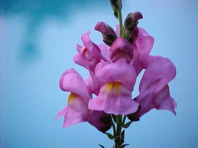
Hariharan, B. and Girshick, R. (2017). Low-shot visual             Torralba, A., Oliva, A., Castelhano, M. S., and Hender-
       recognition by shrinking and hallucinating features. In          son, J. M. (2006). Contextual guidance of eye move-
       Pro. of ICCV, pages 3018–3027.                                   ments and attention in real-world scenes: The role of
He, K., Zhang, X., Ren, S., and Sun, J. (2016). Deep                    global features in object search. Psychological Re-
       residual learning for image recognition. In IEEE Con-            view, 113(4):766–786.
       ference on Computer Vision and Pattern Recognition,         Wang, F., Jiang, M., Qian, C., Yang, S., Li, C., Zhang, H.,
       pages 770–778.                                                   Wang, X., and Tang, X. (2017). Residual attention
Hoffman, J., Gupta, S., and Darrell, T. (2016). Learning                network for image classification. In IEEE Conference
       with side information through modality hallucination.            on Computer Vision and Pattern Recognition, pages
       In Proc. of CVPR, pages 826–834.                                 3156–3164.
Huang, S., Xu, Z., Tao, D., and Zhang, Y. (2016). Part-            Wang, Y., Morariu, V. I., and Davis, L. S. (2018a). Learn-
       stacked cnn for fine-grained visual categorization. In           ing a discriminative filter bank within a cnn for fine-
       IEEE Conference on Computer Vision and Pattern                   grained recognition. In Proc. of CVPR, pages 4148–
       Recognition, pages 1173–1182.                                    4157.
Itti, L., Koch, C., and Niebur, E. (1998). A model of              Wang, Y.-X., Girshick, R., Hebert, M., and Hariharan, B.
       saliency-based visual attention for rapid scene anal-            (2018b). Low-shot learning from imaginary data. In
       ysis. IEEE Transactions on Pattern Analysis and Ma-              Proc. of CVPR, pages 7278–7286.
       chine Intelligence, 20(11):1254–1259.                       Wang, Z., Wang, S., Yang, S., Li, H., Li, J., and Li, Z.
                                                                        (2020). Weakly supervised fine-grained image classi-
Ji, R., Wen, L., Zhang, L., Du, D., Wu, Y., Zhao, C., Liu, X.,
                                                                        fication via guassian mixture model oriented discrim-
       and Huang, F. (2020). Attention convolutional binary
                                                                        inative learning. In Proc. of CVPR, pages 9749–9758.
       neural tree for fine-grained visual categorization. In
       Proc. of CVPR, pages 10468–10477.                           Wei, X.-S., Xie, C.-W., Wu, J., and Shen, C. (2018).
                                                                        Mask-cnn: Localizing parts and selecting descriptors
Kong, S. and Fowlkes, C. (2017). Low-rank bilinear pool-                for fine-grained bird species categorization. Pattern
       ing for fine-grained classification. In Proc. of CVPR,           Recognition, 76:704 – 714.
       pages 365–374.
                                                                   Welinder, P., Branson, S., Mita, T., Wah, C., Schroff, F.,
Krause, J., Stark, M., Deng, J., and Fei-Fei, L. (2013).                Belongie, S., and Perona, P. (2010). Caltech-UCSD
       3d object representations for fine-grained categoriza-           Birds 200. Technical Report CNS-TR-2010-001, Cal-
       tion. In 4th IEEE Workshop on 3D Representation and              ifornia Institute of Technology.
       Recognition, at ICCV, pages 1–8.
                                                                   Xiao, T., Xu, Y., Yang, K., Zhang, J., Peng, Y., and Zhang,
Krizhevsky, A., Sutskever, I., and Hinton, G. E. (2012). Im-            Z. (2015). The application of two-level attention
       agenet classification with deep convolutional neural             models in deep convolutional neural network for fine-
       networks. In Advances in Neural Information Pro-                 grained image classification. In Proc. of CVPR, pages
       cessing Systems, pages 1097–1105.                                842–850.
Kümmerer, M., Wallis, T. S. A., and Bethge, M. (2016).            Xie, G.-S., Zhang, X.-Y., Yang, W., Xu, M., Yan, S., and
       Deepgaze ii: Reading fixations from deep fea-                    Liu, C.-L. (2017). Lg-cnn: From local parts to global
       tures trained on object recognition. arXiv preprint              discrimination for fine-grained recognition. Pattern
       arXiv:1610.01563.                                                Recognition, 71:118–131.
Lin, D., Shen, X., Lu, C., and Jia, J. (2015). Deep                Zhang, H., Xu, T., Elhoseiny, M., Huang, X., Zhang, S., El-
       lac: deep localization, alignment and classification for         gammal, A., and Metaxas, D. (2016a). Spda-cnn: Uni-
       fine-grained recognition. In Proc. of CVPR, pages                fying semantic part detection and abstraction for fine-
       1666–1774.                                                       grained recognition. In IEEE Conference on Com-
Luo, W., Yang, X., Mo, X., Lu, Y., Davis, L., Li, J., Yang,             puter Vision and Pattern Recognition, pages 1143–
       J., and Lim, S.-N. (2019). Cross-x learning for fine-            1152.
       grained visual categorization. In Proc. of ICCV.            Zhang, H., Zhang, J., and Koniusz, P. (2019). Few-shot
Murabito, F., Spampinato, C., Palazzo, S., Pogorelov, K.,               learning via saliency-guided hallucination of samples.
       and Riegler, M. (2018). Top-down saliency detection              In Proc. of CVPR, pages 2770–2779.
       driven by visual classification. Computer Vision and        Zhang, N., Donahue, J., Girshick, R., and Darrell, T. (2014).
       Image Understanding, 172:67–76.                                  Part-based r-cnns for fine-grained category detection.
Nilsback, M.-E. and Zisserman, A. (2008). Automated                     In European Conference on Computer Vision, pages
       flower classification over a large number of classes. In         834–849.
       Sixth Indian Conference on Computer Vision, Graph-          Zhang, X., Xiong, H., Zhou, W., Lin, W., and Tian, Q.
       ics & Image Processing, pages 722–729.                           (2016b). Picking deep filter responses for fine-grained
Pan, J., Canton, C., McGuinness, K., O’Connor, N. E., Tor-              image recognition. In Proc. of CVPR, pages 1134–
       res, J., Sayrol, E., and Giro-i Nieto, X. a. (2017). Sal-        1142.
       gan: Visual saliency prediction with generative adver-      Zheng, H., Fu, J., Mei, T., and Luo, J. (2017). Learning
       sarial networks. In arXiv.                                       multi-attention convolutional neural network for fine-
Sun, M., Yuan, Y., Zhou, F., and Ding, E. (2018). Multi-                grained image recognition. In Proc. of ICCV, pages
       attention multi-class constraint for fine-grained image          5209–5217.
       recognition. In Proc. of ECCV, pages 834–850.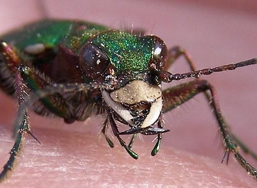
You can also read