Market effiency in Finnish harness horse racing - Keskustelualoitteita #65 - Niko Suhonen - UEF ...
←
→
Page content transcription
If your browser does not render page correctly, please read the page content below
Keskustelualoitteita #65
            Joensuun yliopisto, Taloustieteet

Market effiency in Finnish harness horse racing

                 Niko Suhonen

               ISBN 978-952-219-283-7
                  ISSN 1795-7885
                       no 65
Market Efficiency in
Finnish Harness Horse Racing
Niko Suhonen *
University of Joensuu
(niko.suhonen@joensuu.fi)
August 2009
Abstract
The paper analyzes the efficiency of the betting markets in Finnish
harness horse racing. We first present the basic properties of the
betting markets. We focus on the organization structures, the market
efficiency, and the well-known inefficiencies. Next we review
different methods to test the market efficiency. An alternative method
proposed based on actual and on theoretical net returns is introduced.
Finally the betting market efficiency is tested with different tests using
database accumulated from the Finnish harness horse race tracks.
Robustness of results is controlled with bootstrap methods. The results
imply that the markets are semi-strong efficient and characterised by
the favourite long-shot bias. However, consistent evidence for other
game market anomalies like end of the day effect or gambler’s fallacy
is not found.
*
I thank Mika Linden, Timo Kuosmanen, and Tuukka Saarimaa for their helpful comments and suggestions. I also wish
to thank Jani Saastamoinen for providing data. Financial support from Yrjö Jahnsson Foundation, Finnish Cultural
Foundation, and The Finnish Foundation for Gaming Research is gratefully acknowledged.
11. Introduction
Gaming is a large business, and the general attitudes for gambling have been liberated from the
curtain of sin. Nowadays, betting is more acceptable and it can be seen as entertainment. However,
the political discussion about the market structures in gaming is passionate. Typically, in many
European countries gaming is organized by full legal monopolies. However, the pressure to open
the market for free competition widens everyday.
Free competition in the betting markets may lead to richer gambling menus and even lower prices at
least in some gambles. On the other hand, gaming and its problems, such as gambling addictions,
may easier be controlled by a monopoly. However, we do not take policy approach. Instead, we
examine how gamblers behave in these markets.
Our first aim is to briefly discuss market efficiency conditions and different testing methods in
betting markets. Secondly, we introduce an alternative testing method in which the confidence
intervals for net return rates are calculated with bootstrap methods to secure more appropriate
statistical testing. Finally, we test how efficient the Finnish harness horse race betting markets are.
The paper is organized as follows. In section 2, we take a look at some the key properties of betting
markets such as the organization structures, the market efficiency, and the well-known
inefficiencies. Next, we present the methods used to test the betting market efficiency. Section 4
includes descriptions of our dataset and assumptions. In section 5, we introduce our method. The
empirical results from the different test types are presented in section 6. The last section concludes
the paper.
2. Market Efficiency in Betting Markets
2.1 How Betting Markets Work?
There are a lot of similarities between financial markets and gambling markets. For instance, both
of these markets have a large number of investors or bettors that have an opportunity to access the
set of information, which may help to predict an outcome of the game. However, there are also
differences. In the gambling markets bettors do not have an opportunity to sell their ‘ticket’ in a
secondary market. Moreover, gambling markets constitute an environment that has targeted
investments and fast profit clearance. This is different compared to the financial markets at least
some of them. For a more precise discussion of similarities between gambling and financial
markets, see e.g. Sauer (1998).
2Although financial and gambling markets are analogous, there exists one conceptual difference: the
enjoyment of gambling. Gambling brings positive (enjoyment) consumption for the gamblers and
they are also prepared to pay for it. However, in both markets gamblers try also to maximize
(minimize) their profits (losses) or utility.
As consumption of gambling is part of gambling, the gambling markets include both the demand
and supply side. Gamblers are the consumers that ask for the gambling service. Typically the
bookies offer game opportunities based on some sport event or in lotteries. Bookies will return the
gamblers an amount of money that is dependent, at least at some level, on the probability of the
outcome. There are two main traditions to organize the supply side: pari-mutuel and bookmaker
mechanism. In pari-mutuel system (or totalizator) gamblers’ winning bets share the pool of all bets.
Thus, the pool shares constitute the odds for every possible outcome and the odds determine the
payoffs for the gambler. However, the odds are not directly contractual after betting. For instance, if
the gambler bets five minutes before closing time, it is possible that the odd varies because of the
other gamblers’ betting behaviour. Therefore, the final odd and the payoff are fixed when the
betting is closed. In the pari-mutuel system, the operator takes a share of the pool to cover the costs,
taxes and profits. This is the so-called take-out rate and it decreases the odds and payoffs.
Therefore, the established pari-mutuel system is risk-free for the operator. Actually the bettors
gamble against each other.
The bookmaker system operates somewhat differently. In this system, the bookmaker offers fixed-
odds to the bettor. This means that the bettors know for sure their possible payoffs after
participating, although the bookmaker can offer different odds after gamblers’ decision. For this
reason, if the betting volumes go ahead in some direction, the bookmaker tries to equalize the
betting volumes by changing the odds. Therefore, even the bookmaker offers odds independently,
the decisions are affected by the gamblers betting behaviour. Due to the bookmaker system, the
operator has some risk and bettors gamble directly against the bookie. Similarly as in the pari-
mutuel system, the bookmaker’s take-out rate decreases the odds.
In general, both systems are used in horse race track betting. For instance, pari-mutuel system is
used in the North America, France, Germany, Japan, Hong Kong and Finland. Respectively, the
betting markets are organized by a bookmaking system at least in the Great Britain and Australia.
As the odds are inversed winning probabilities adjusted by the take-out rate, the probabilities reflect
market information. Odds in the pari-mutuel system equal the gamblers’ subjective probabilities.
3Contrary to this, the bookmaker’s odds reflect both his own and gamblers’ estimations of winning
probabilities. This builds up the simultaneous supply and demand for a game price in ex-ante sense.
If all available information used efficiently this “market price” is close to the true ex-post odds, i.e.
a market is expected to operate efficiently. Now, as we have historical information concerning the
past game outcomes and odds related to particular horses, we can test in ex-post sense how correct
these market estimations have been. Thus we can test how efficient or unbiased the horse race
betting markets are.
2.2 Definition of Market Efficiency
For now on, we discuss the pari-mutuel horse race track betting in which the market information
plays a crucial role. Thus, the odds and the bettor’s subjective probabilities refer to the gambling
market’s estimates of each horse’s chance of winning the race and these odds can be used to
analyze the betting market efficiency. Market efficiency has several concepts and definitions. Next
we proceed with the definition by Thaler & Ziemba (1988). The following three definitions of the
market efficiency (ME) seem appropriate 1 .
1. Weak ME: Does the subjective probability predict the objective probability?
2. Semi-strong ME: Do some systematic bets have positive expected value?
3. Strong ME: Does every bet have the same expected value?
In finance, market efficiency analysis is based on the following conditional (rational) expectation
hypothesis
Pt 0+1 = E[ Pt +E1 | Ωt ] ,
where Pt 0+1 is the observed market price at next period and E[ Pt +E1 | Ωt ] is conditional expectation
(prediction) for it based on the relevant present and past market information Ωt . The efficiency
condition is also formulated in following way E[ Pt 0+1 − E[ Pt +E1 | Ωt ]] = 0 , i.e. no systematic prediction
errors exist. In the context of game markets we can give a similar example that illustrates the basic
relation between subjective probability and objective probability. The market efficiency conditions
1 (ME1) and 3 (ME3) can be analyzed with the following simple regression model
1
In fact, Thaler and Ziemba (1988) used only conditions 2 and 3. However, we added the condition 1 for a logical
clarification.
4Objective probabilityi ,t = β 0 + β1Subjective probabilityi ,t + ε i ,t , (2.1)
where E[ε i ,t ] = 0 for ∀i, t .
The condition ME1 is almost trivial as subjective and objective probabilities are highly correlated.
Thus, if β1 > 0 , then we can say that the implicit odds predict in average the true winner in the
correct direction. Condition ME3 is more informative. If every bet has the same expected value or
each bet’s expected value is known, then the subjective probability should predict the objective
probability without bias for ∀i , i.e. β 0 = 0 and β1 = 1 . Equation (2.1) does not give a direct answer
to condition ME2. However if it is possible to reach a positive expected value with systematic
betting then β 0 ≠ 0 and β1 > 0 .
Testing the betting market efficiency seems to be straightforward but the main problem is to have
an appropriate estimate for the objective probability in horse race betting. For instance, the lotto
game and the horse race betting differ fundamentally from each other 2 . However, if we have
enough historical data from the horse race betting for a particular horse, we can estimate the
objective probabilities that give us some tools to make comparisons. In Section 3, we discuss the
estimation methods in details.
2.3 Well-known Inefficiencies
The best-known and documented inefficiency in the gambling markets is the Favourite-longshot
Bias: the favourites are under-bet while the long-shots are overbet (FLB for short)3 . As a result, if
gamblers bet systematically for the favourites, they do not lose as much as gamblers that prefer the
longshots. In the pari-mutuel system, this phenomenon clearly reflects the gamblers’ behaviour.
However, FLB is also manifested in the bookmaker market as well, and, therefore, it is probably
affected by both the demand and supply side elements. For the survey of FLB, see, for instance,
Thaler & Ziemba (1988), Sauer (1998), Coleman (2004).
We illustrate by a Finnish horse racetrack dataset how FLB contributes to the gambler’s expected
returns. Figure 1 shows that the rate of net return (RR) on betting horses with high odds (60-70) is
2
The most lotto games use the pari-mutuel system but the objective probabilities for every winning outcome are known.
Thus, in theory, it is possible to calculate the exact payoff for every outcome if we have information about gamblers
betting behaviour.
3
The bias was first noted by Griffith (1949).
5between -40% and -50%, and betting of favourite yields losses only about -15%. Theoretical loss –
the take out rate - is about -20%.
Figure 1. Odds and the rate of net returns.
The Finnish data illustrates very well race track studies around the world from the 1950s to the
present day, with very few exceptions. Ziemba (2008) notices that FLB has slightly weakened in the
course of time. However, there is no evidence that FLB has vanished from the racetracks (i.e., the
markets have come efficient in the long run). Note that Kanto et al. (1992) have previously studied
Finnish horse racetrack betting. They used a dataset from Teivo racetrack in Tampere that covered
40 racing days from the autumn 1986 to the summer 1987 with a total of 395 harness races.
However, they used a double betting dataset instead of a win betting data to analyse FLB. 4 They
found evidence for FLB.
Formally, FLB is valid in the Equation (2.1) when β 0 < 0 and β1 > 1 . Thus, the large probabilities
are over weighted and the small probabilities are under weighted. However, although FLB is
generally accepted, Busche & Hall (1988) found that FLB is not valid in Hong Kong. Busche
(1994) confirmed this by dataset from Japan and Hong Kong. These results are important because
4
Double bets means that the gamblers have to choose two horses finishing first and second irrespective order and it is
identical quinella betting in the North America.
6Busche & Hall (1988) actually found evidence for the opposite: the large probabilities are under
weighted and the small probabilities are over weighted (i.e. β 0 > 0 and β1 < 1 ).
What explains bettor’s systematic behaviour? Two main explanations have emerged in the
literature. Bettors have 1) a risk-love utility function, and/or 2) a biased view of probabilities. Note
also that Shin (1991, 1992, 1993) showed that the presence of insiders can generate FLB in the
betting markets. 5
If the gamblers (in representative sense) are risk-lovers, they prefer to bet for horses that have a
small probability of winning, i.e. a high payoff. Thus, they are prepared to pay more to generate
their utility or enjoyment compared to the risk-aversive or risk neutral gamblers, which are not
willing to participate the gamble at all (in that case, the word ‘bias’ is somewhat misleading.)
Weizman (1965) estimated utility function for an average expected utility maximizer. He found that
the convex utility function explains gamblers’ behaviour, consistent with the assumption of a risk-
love attitude. After Weiztman (1965), for instance, Ali (1977), Golek & Tamarkin (1998) and
earlier mentioned Kanto et al. (1992) confirmed the risk-love attitude utility function.
Alternatively if bettors have misperceptions of probabilities in the sense that they undervalue the
high probabilities and overvalue the small ones, favourite-longshot bias results are obtained. This
was Griffith’s (1949) explanation for the phenomenon. Note that the Prospect Theory (Kahneman &
Tversky 1992, 1979) takes the biased view of probabilities as a fact. Thus, it can be argued that
FLB has nothing to do with risk attitude. The question is about the misperception of probabilities.
To make a difference between these two approaches is difficult. Snowberg & Wolfers (2007)
showed by their win betting dataset that the both approaches are justified. CARA utility function
with risk-love fits the data reasonably well. Similarly, estimating a probability weighting function
proposed by the Prospect Theory fits the data equally well. 6 Thus, there is nothing in the win
betting data that allows the econometrician to distinguish between risk-love and misperception.
However Snowberg & Wolfers (2007) used the win betting data and the exacta (two horses
finishing in exact order), trifecta (three horses finishing in exact order), and quinella (the gamblers
have to choose two horses finishing first and second irrespective order) datasets also in their
5
See more explanations, e.g., Sauer (1998).
6
Although the Prospect Theory suggest two parameter weighting function, they used one parameter function by Prelec
(1998) in estimation.
7analysis. Although these datasets have similar problems as the win betting data, their comparison is
illuminating. Thus, Snowberg & Wolfers (2007) estimated first both the risk-love model and the
misperception model with the win betting data. Then they predicted the exacta, quinella and trifecta
datasets’ records with these models and compared fitted models with true records. As a result, they
noticed that FLB is consistent being driven by the misperception rather than the risk-love model.
Moreover, they argued that the results suggest that non-expected utility theories (e.g., the Prospect
Theory) are a promising candidate for explaining racetrack bettor behaviour.
However, efficiency test values can be harmed also by other type inefficiencies. End of the Day
Effect (EDE) is interesting, although not extensively documented, regularity. In EDE gamblers’
behaviour changes to more aggressive in the last races of the day. In practice, this means that FLB
is especially strong in the last races (see McGlothlin 1956, Ali 1977, and Asch et al. 1982). This is
consistent with the assumption of the Prospect Theory that bettors are loss-aversive and risk-lover
below the reference point. Most bettors are losing in the end of the day and the last races give the
opportunity to win back their money. However, Snowberg & Wolfers (2007) does not confirm EDE
in their large dataset.
Gambler’s Fallacy (GM). The bias is an incorrect belief of the probability of an independent event
when the event has recently occurred many times. This is well documented in experiments and in
real gambling markets as well. For instance, Clotfelter & Cook (1991) noticed that in the lotto
gambling, gamblers rarely chose the number which occurred in the previous round. Croson &
Sundali (2005) conducted the field experiment in casinos (roulette) and found the evidence that
supports the assumption of the gambler’s fallacy. In the case of pari-mutuel horse race betting, the
gambler’s fallacy hypothesis can be stated as follows. Bettors underestimate the probability of the
favourite horse if it has won the previous race. Metzger (1985) conducted a study in which she
validated some support of the gambler’s fallacy: betting on the favourites decreases with the length
of their run of success. Moreover, Terrell & Farmer (1996) used the dog race data. They noticed
that betting for the winning dog from the previously track will even constitute a profitable betting
strategy.
83. Methods of Testing Inefficiency
3.1 Basic Definitions and Notations
The following definitions are employed. The odds, Oi , are derived from the gambler’s bets in each
race. Thus, Oi for the horse i can be written as
−1
⎛ b ⎞
Oi = ⎜ ni ⎟ (1 − τ 0 ) , (3.1)
⎜ ∑ bi ⎟
⎝ i =1 ⎠
∑ b is the sum of bets for all n horses, and τ 0 is the take-
n
where bi is all bets for the horse i , i =1 i
out rate. Respectively, the average or representative subjective probability for horse i is
⎛ 1 ⎞
ρi = ⎜ ⎟ (1 − τ 0 ) . (3.2)
⎝ Oi ⎠
The rate of net return for a one-euro bet is
E ( Ri ) = pi Oi − 1 , (3.3)
where pi is the true winning probability of horse i . Now, if the subjective probability and the true
probability are equal, then the rate of net return is the take-out rate ( −τ 0 ), and the strong market
efficiency condition 3 is established. However, to test this condition we need, like the bettors need,
an unbiased estimate of objective probability.
3.2 Different Methods of Estimating (In)efficiency
There are three different techniques to tackle the issue: 1) grouping by favourite positions, 2)
grouping by the pari-mutuel odds, and 3) regressing the net return by the odds. These are the
methods used since the 1950’s. Next we briefly review these methods.
Grouping by favourite positions. The method was first used by Ali (1977). First, we rank horses
into groups (h) by the favourite position in every race: the favourite horse is group one, and so on.
Second, suppose that π h is an objective winning probability for a horse, which was included in
9group h . The objective probability for group 1 (the favourite) is calculated by dividing all winning
cases of group 1 with all races. Formally, it can be represent by
∑
m
j =1
Y jh
πh = , h = 1, 2,..., H (3.4)
m
where Y jh = 1 , when a horse in group h wins the race j , and otherwise zero. A number of races is
m . Notice that Y jh is a Bernoulli variable. Because the races are independent, Y jh is Binomially
distributed. Moreover, the estimators of expectation and variance of Binomial distribution have the
following unbiased properties: E (Y jh ) = π h and Var (Y jh ) = π h (1 − π h ) / m . Furthermore, the
subjective probability in each group h can be calculated by
∑ ρ jh
m
j =1
ρh = , h = 1,..., H . (3.5)
mh
The test for gambling biases is H 0 : ρ h − π h = 0 for all h = 1,..., H , i.e. are the subjective and
objective probabilities in different groups equal. We can approximate the Binomial distribution by
the Normal distribution if the observation sample is large enough. According to the the Central
Limit Theorem
ρh − π h
zh = ∼ N (0,1) . (3.6)
π h (1 − π h ) / m
While this technique is very simple there are also problems in using it. First, the subjective and the
objective probabilities have distributions of their own, and they have also distribution specific
standard errors. However, in Eq. (3.6) we have assumed that the subjective probability is a constant.
Second, we assume that the favourite positions in all races are Bernoulli variables. However, there
are high variations in the race circumstances (e.g., jockey, contenders, weather etc.). Basically, the
nature of probability estimation for a horse is something else than, for instance, estimating objective
probability of heads in an experimental coin toss trial. The violation of random experiment
10assumption may bias the objective probability estimate and its standard error 7 . However, the
problem of variations of objective probability can be partly avoided by using odds segments.
Grouping by the pari-mutuel odds. This is the approach first used by Griffith (1949), and followed
by, for instance, Snyder (1978), and Jullien & Salanie (2000). The basic structure of the method is
close to favourite position analysis but now all information on the odds is used. We divide the
betting data (horses) into ‘nearby’ equal-sized groups by the odds levels (e.g. 1.0-1.5), and the
objective probability is the proportion of horses with odds group that won their races (similarly as
in Eq. (3.4)). 8 The benefit of this method is that the variation of the odds is now controlled.
Respectively, the subjective probability is calculated similarly as in Eq. (3.5) while the rank is
changed to the odds group. Now we can use estimates of the objective and the subjective
probabilities to analyze the regression model (Eq. (2.1)). Thus, if we use estimates of the favourite
grouping process, we have H number of observations. Similarly, the grouping method by the odds
gives us number of observations that are equal to the number of odds group chosen. However, Ali
(1977) noticed, and Busche & Hall (1988) later discussed, that identity of a single horse is lost in
above practices, i.e. in the odds group includes several horses but only one win. Thus, the estimate
of the objective probability is somewhat undervalued. Moreover, the aggregation in both methods
may introduce a bias as well.
Regressing the net return by the odds. Vaughan Williams & Paton (1998) responded to the critique
of the grouping methods by regressing the net return by the odds. In this analysis, the actual return
for a unit stake on each horse is calculated. In practice, if the horse loses, the return is equal to -1
euros and, in turn, if the horse wins, the return is equal to the net return Ri = Oi − 1 . Therefore we do
not need to make any groups and avoid the problems of categorizing. However, the dependent
variables, the net returns, are left-censored at -1. Consequently, the OLS estimates are biased and
Censored or Tobit estimation is more appropriate alternative. Moreover, the returns for horses
within a given race are not independent. Because of this the clustered Tobit estimation by race is
used. In this context the regression model is
Rij = α 0 + α1Oij + uij , (3.7)
7
We will discuss this topic more precisely in the next section.
8
The procedure of building the odds groups seems not to affect the results. For instance, Gandar et al. (2001) conclude
that results were similar if they used even-sized odds categories or even numbers of horses in each odds category.
11where Rij is the actual net return to a unit bet on the i th horse in the j th race, Oij is the horse’s
odds, and uij is an error term with zero expectations. Because of the take-out rate, the net returns
are expected to be negative with all odds level according to the condition ME2. That is, we have
α 0 < 0 . In addition, the existence of FLB indicates that the net returns are lower (higher) for higher
(lower) odds levels of horses implying that α1 < 0 .
4. Alternative Approach to Examine (In)efficiency
4.1 Background and Motivation
The categorisation procedures, especially favourite position method, may produce some bias and
measurement errors in the probability estimates. To motive our alternative method we illustrate the
problems found above as clearly as possible with our Finnish dataset. In the favourite position
method the variation of odds does not matter, therefore, calculating the rate of net return by this
information is somewhat ambiguous. Remember that subjective probabilities are based on odds
information but the objective probabilities are not.
Figure 2a presents favourites (rank 1) odds distribution in all races. Respectively, Figure 2b shows
odds distribution for the favourite which have actually won the race.
3,600 2,000
3,200
2,800 1,600
2,400
1,200
2,000
1,600
800
1,200
800 400
400
0 0
1 2 3 4 5 6 7 1 2 3 4 5 6 7
Odds Win Odds
Figure 2a. Odds distribution of rank 1. Figure 2b. Win odds distribution of rank 1.
We can notice that both distributions are slightly skewed to the right but with a larger extension for
the win odds distribution. This is obvious because horses with low odds win more probably.
However, as we know that the objective probability is the ratio of number of wins with a favourite
12position to number of races, the win odds distribution is redundant. Thus, the rate of net return
calculated only by favourite odds information will lead to biased results. 9
Note that if we use the odds grouping method, the variation of odds can be controlled with odds
intervals. A thin (wide) interval will minimize (maximize) the variation. Consequently, with the thin
margin the bias is low, although not completely vanishing. Alternatively, we can simply calculate
all bets on the favourite and compare this with the actual winning returns. Formally this may be
written as
Sum of Bets on Rank (h) − Sum of Rank (h) Returns
E ( Rh ) = . (4.1)
Sum of Bets on Rank (h)
Thus, the problems mentioned above can be handled to some extension. However, the questions
“What is the true relation between the objective and the subjective probability” still remains.
Naturally, it would be appropriate that there were not any controversial arguments, for instance, on
the definition of objective probability even FLB is an evident phenomenon irrespective of
measurement method. Next, we show that an alternative method that will end up at the same
conclusion, but from a different point of view.
4.2 Alternative Approach
The previous aggregation methods were based on estimating the probabilities. In turn, our approach
focuses on the returns of bettors, and indirectly ignores the probabilities. We still keep with the
favourite position method but instead estimating the objective probabilities, we estimate the
theoretical value of return of the horse based on historical horse racing results.
To understand the procedure consider the win odds (average), WOh , in every rank category h. The
win odds are actually materialized and we have a vector of win odds for each rank. Moreover, these
different win odds categories have their own distributions like in Figure 2b. Consequently, the
expected rate of net return for 1 euro bet for rank h can be written as
E ( Rh ) = π hWOh − 1 , (4.2)
πh
9
Note that calculating the rate of net return by E ( Rh ) = (1 − τ 0 ) − 1 , is biased as well.
ρh
13which constitutes a parallel result with the Eq. (4.1). Note that the objective probability does not
affect win odds WOh . The probability is constant by nature because bettors cannot influence it.
Contrary to this, the win odds are directly affected by bettors.
The approach leads to questions: Are winning odds line with theoretical assumptions of market
efficiency? The answer to this question is two fold. Firstly, if we assume that bettors behave as
rational risk neutral gamblers with unbiased view of probabilities, their expected loss or rate of net
return is −τ 0 . This should be valid in every rank category. That is
E ( R1 ) = E ( R2 ) = ... = E ( RH ) = −τ 0 . (4.3)
Secondly, according to this assumption, the theoretical or objective (average) of win odds in every
category can be calculated by Eq. (4.2)
1 −τ 0
WO*h = . (4.4)
πh
Next we illustrate the idea in Figure 3 10 . Figure shows how the market efficiency conditions are
determined with win odds procedure. First, actual win increases with the theoretical value,
condition ME1 is valid. Second, if the actual wins do not exceed break-even, condition ME2 is
effective also. Finally, when the wins are higher for favourites (grey area) and lower for longshot
(black area) than for the theoretical win odds, the condition ME3 ( β 0 = 0 and β1 = 1 ) is
systematically violated. The FLB result is evident.
Our testing strategy is whether the theoretical win odds are equal to actual win odds in each rank
category. Typically, we could test the equality of theoretical wins and the win odds by using
information on the win odds’ standard errors and normal distribution assumption. In that case, our
hypothesis can be written as
H 0 : WOh* = WOh
H1 : WOh* ≠ WOh .
10
The idea to Figure 3 is adapted from the Busche & Hall (1988).
14Figure 3. The market efficiency conditions with win odds.
Now, a confidence interval based on WOh as described above is
WOh − z1−α / 2 [ se(WOh )] < WOh* < WOh + z1−α / 2 [ se(WOh )] , (4.5)
where se( WOh ) is the standard error and z1−α / 2 is the value from the N(0,1) distribution with excess
of probability 1 − α / 2 . The usual values for α are 0.10, 0.05 and 0.01. H 0 is rejected if
WOh exceeds the upper limit or is less than the lower limit.
However, as we saw in Figure 2b the win odds are not normally distributed. This rises the question
of the appropriate confidence intervals of equality tests. Thus, the conventional statistical
interference can be misleading. To secure the robustness of the results, we estimate the confidence
intervals for each rank category by Bootstrap, and particularly with the percentile method. First, we
compute 10,000 bootstrapped samples from the win odds data by randomly sampling with
15replacement. For each bootstrapped sample, we compute mean, WOˆ hb , and sort them from the
smallest to the largest value. Consequently, the 99 % confidence interval can then be estimated
simply by selecting the bootstrapped statistics at the low 0.5-th and high 99.5-th percentiles.
Furthermore, in a two-tailed test,
H 0 : WOh* = WOh is rejected if WOh* ≤ WOˆ hb ,low or WOh* ≥ WOˆ hb ,high .
According to the bootstrapped confidence intervals, we can calculate confidence intervals to the
actual rate of net returns which can be written as
π hWOˆ hb ,low − 1 = E ( Rhlow ) and (4.6)
π hWOˆ hb ,high − 1 = E ( Rhhigh ) . (4.7)
Finally, if the take-out rate −τ 0 is between the above confidence intervals, the condition ME3 and
Eq. 4.3 are established.
5. Data Descriptions and Necessary Assumptions
Our dataset is provided by Suomen Hippos (the Finnish Trotting and Breeding Association)
WebSite with computer programme. In Finland, Suomen Hippos has a monopoly, by law, to
organize pari-mutuel betting in horse racing (harness), and the total yearly turnover is over 140
million euros. There are 44 racetracks in Finland and the main track of the country, Vermo, is
situated in Helsinki, and it hosts over 60 race events every year. The gambling menu covers the
traditional Win, Show and Quinella betting types that can be bet on every race. Trifecta, as well as
Superfecta, can be bet on particular races. There is possible off-track betting. Moreover, betting on
almost every race in Finland via the internet is possible. The tote’s take-out rate on average is 20.97
% (calculated from the dataset).
The dataset includes win betting information and consists of horse race runs in Finland from
3.1.2002 to 19.7.2007. On the whole, the data includes 27,595 harness races, and the total number
of included horses is 345,308. Thus, our data contains odds for the horses in every race and
information on the exact finishing order of horses. We dropped out the races in which numbers of
running horses was under ten. Moreover, if the take-out rate was an obvious outlier (i.e. too high or
16low), we dropped also the race out of the data. The data does not contain any information about the
characteristics of an individual bettor or average amounts of the bet per race per person. Therefore
we assume an agent or a bettor that typifies all the bettors, the so-called representative bettor. 11
6. Results
6.1 FLB with Different Tests
We replicated different test types for FLB by using Finnish dataset. First, the results of grouping by
favourite positions test (Eq. 4.6) are shown in Table 1. The results confirm the FLB. Favourites are
under bet while long-shots are over bet. The cross point is in the 4th and 5th ranked horse, in which
the difference between the objective and the subjective probability is not statistical significant.
These results are line with the previous studies.
Table 1. Objective and subjective probabilities by favourite position.
Rank No. races No. wins Average Odds Subjective Objective Standard z-value
Probability Probability Deviation ( ρh − π h )
1 27595 9734 2.71 0.3260 0.3527 0.002876 -9.31***
2 27595 4865 4.96 0.1731 0.1763 0.002294 -1.42*
3 27595 3359 7.23 0.1185 0.1217 0.001968 -1.63*
4 27595 2460 9.74 0.0886 0.0891 0.001715 -0.31
5 27595 1863 12.66 0.0690 0.0675 0.001510 0.97
6 27595 1419 16.08 0.0550 0.0514 0.001330 2.66***
7 27595 1040 20.31 0.0442 0.0377 0.001146 5.68***
8 27595 901 25.52 0.0357 0.0327 0.001070 2.84***
9 27595 691 32.41 0.0287 0.0250 0.000941 3.87***
10 27595 480 42.04 0.0227 0.0174 0.000787 6.73***
11 23774 359 51.19 0.0186 0.0151 0.000791 4.41***
12 17383 204 58.93 0.0159 0.0117 0.000817 5.08***
13 10707 123 63.16 0.0144 0.0115 0.001030 2.85***
14 8815 79 73.03 0.0121 0.0090 0.001004 3.15***
15 6077 45 81.60 0.0105 0.0074 0.001100 2.80***
16 2602 15 88.29 0.0094 0.0058 0.001484 2.45*
* Indicates that the difference is significant at the 10 % level, ** at the 5 %, *** at the 1 %.
Note that rank positions are in logical order, i.e., number of winnings decrease monotonically with
the rank positions. This is, indeed, a necessary assumption for the method but at the same time it
supports validity of the ME1 condition. Moreover, since we have a data on the exact finishing
order for every horse, we can check the link between rank and finishing position (e.g. did the horse
ranked 4th really finished the line in 4th place). In most cases the rank positions predicted finishing
positions quite accurately. The finishing positions were slightly distorted at the top places. This is
11
Naturally, racetrack bettors have heterogeneous preferences and information.
17due to the fact that in the harness races disqualifications and interrupts are very common. However,
there does not seem to be any systemic violations that prevent the use of rank positions method.
As the grouping by odds positions method leads to the identical results, we do not present the exact
results in here. However, we made regression on objective probabilities implied by Eq.(2.1). We
used the data from the grouping by odds position. Results from the regression are shown in Table 2
Table 2. OLS estimates of the probabilities.
Dependent Variable: Objective Probability with the restrictions β 0 = 0 and β1 = 1
Coefficient Std. Lower 99 % Upper 99 %
Error Confidence Interval Confidence Interaval
Constant -0.0122** 0.00193 -0.01700 -0.00749
Subjective Probability 1.1376** 0.01433 1.10227 1.17295
No. Obs. 29
R2 0.99
** Significant at the 1 % level.
The analysis gives clear and unambiguous answers to market efficient conditions ME1 and ME3.
Bettors’ subjective probability valuations predict actual outcomes. However, the strong efficiency is
violated. Subjective expectations do not equal the objective outcomes, and the markets are
systemically characterised by FLB.
Next we Tobit regress net returns on odds (i.e. Eq. 4.7). Our main findings are presented in Table 3.
Table 3. Clustered Tobit regression estimates for net returns.
Dependent Variable: Net Return
Coefficient Std. Error Slope
Constant -21.30** 0.3792 -
Odds -0.4878** 0.0048 -0.0606
No. Obs. 345308
Clusters 27595
Standard Error 20.93
Log-Likelihood -176196.4
Note: Standard errors are Huber/White robust estimates. ** Significant at the 1 % level.
Now, constant is negative ( α 0 < 0 ). Thus, at the first place it indicates that there is no opportunity
of systematic winning strategy and the take-out rate makes betting unprofitable for the gambler.
Moreover, the second estimate is also negative ( α1 < 0 ). Therefore, when the odds increase the net
18returns decrease. FLB is evident by this method as well. Note that Tobit estimates require adjusting
before they can be interpreted as marginal effects. The correct marginal effect (slope) is estimated
following Greene (2003). Slope is -0.061. It suggests that an increase in the odds of one unit
decreases the expected net return of one-euro bet by six cents. The Tobit regression method gives
answer also to the condition ME2. There are not systematic bets that have a positive expected
value. For the comparison, Gandar et al. (2001) examined New-Zealand thoroughbred pari-mutuel
horse races (117,775 observations), and their results were similar to ours. Thus there seems not to
be any cultural differences in results.
In summary, Finnish horse race betting markets are efficient in semi-strong level: odds reflect the
outcomes of the races and there is not opportunity to make any profits by simply systematically
betting without extended information. However, the assumption of the strong efficiency condition
EM3 is rejected and the market is characterised by FLB.
6.2 Market Efficiency with Alternative Method
Next, we present our results of testing FLB that is based on the alternative method. Table 4 includes
basic information about estimates and bootstrapped confidence intervals.
Table 4. Actual win odds, theoretical win odds, and confidence intervals.
Bootstrapped Bootstrapped Bootstrapped Bootstrapped
Win Lower 99 % Upper 99 % RR Lower RR Upper
Win Theoretical Conf. Conf. Actual 99% Conf. 99% Conf. Sum of
Rank Odds Odds Interval Interval RR Interval Interval Wins
1 2.41 2.24 2.38 2.43 -0.151* -0.159 -0.143 23426.1
2 4.52 4.48 4.48 4.57 -0.203 -0.211 -0.194 22004.3
3 6.56 6.49 6.48 6.64 -0.202 -0.211 -0.192 22026.4
4 8.82 8.87 8.68 8.96 -0.214* -0.226 -0.201 21694.1
5 11.17 11.71 10.98 11.37 -0.246* -0.259 -0.232 20811.2
6 13.90 15.37 13.61 14.21 -0.285* -0.300 -0.269 19726.7
7 17.35 20.97 16.90 17.83 -0.346* -0.363 -0.328 18045.2
8 21.69 24.20 20.99 22.43 -0.292* -0.315 -0.267 19538.6
9 26.68 31.56 25.70 27.79 -0.332* -0.357 -0.304 18436.8
10 32.71 45.43 31.08 34.45 -0.431* -0.459 -0.401 15699.2
11 41.35 52.34 38.96 43.87 -0.376* -0.412 -0.338 14843
12 46.91 67.34 43.53 50.65 -0.449* -0.489 -0.406 9569.9
13 50.44 68.79 45.72 55.32 -0.421* -0.475 -0.364 6204
14 62.49 88.18 56.09 69.15 -0.440* -0.497 -0.380 4937.1
15 74.98 106.72 66.39 82.85 -0.445* -0.508 -0.387 3374.2
16 79.55 137.09 66.61 91.55 -0.541* -0.616 -0.472 1193.3
Note: Table 1 shows other information about ranking procedure (e.g., number of races and wins). The confidence
intervals for the rate of net return are calculated by the bootstrapped win odds intervals as mentioned in Section 4.2.
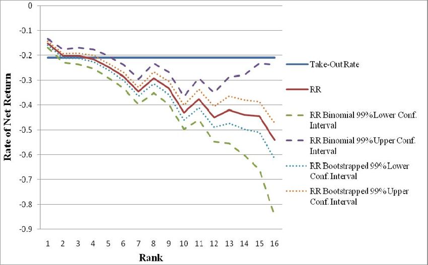
19The theoretical rate of net return or take-out rate is -0.209, and it fits only the bootstrapped
confidence interval of the groups two and three. Clearly, FLB is true regardless the method but the
alternative method is more precise compared to the favourite position method with binomial
distribution assumptions. Figure 4 illustrates the difference between the tests with the confidence
intervals of the rate of net returns. The intervals of the rate of net returns calculated by the Binomial
distribution assumptions are wider than the bootstrapped ones. However, we adhere to our method
and test other efficiencies as well. 12
Figure 4. Binomial and bootstrapped confidence intervals of the rate of net returns.
End of the Day Effect. Next we test for the end of day effect. We did the same calculations as above
but only information of day’s last races was used. Table 5 shows the results. The confidence
intervals for the rate of net return are calculated by the bootstrapped win odds intervals in the all
races.
12
We also compared the bootstrapped confidence intervals and the Normal distribution confidence intervals based on
win odds information. Surprisingly, the results were very similar. The exact results are shown in Appendix 1.
20Table 5. Winning odds, the net rate of returns and confidence intervals for the day’s last race.
RR Last Bootstrapped RR Lower Bootstrapped RR Upper
Rank No. Wins Win Odds Race 99% Confidence Level 99% Confidence Level
1 1089 2.48 -0.142(H) -0.159 -0.143
2 522 4.52 -0.251(L) -0.211 -0.194
3 360 6.58 -0.248(L) -0.211 -0.192
4 278 8.84 -0.220 -0.226 -0.201
5 218 11.00 -0.238 -0.259 -0.232
6 180 14.10 -0.194(H) -0.300 -0.269
7 134 16.62 -0.293(H) -0.363 -0.328
8 120 21.30 -0.188 (H) -0.315 -0.267
9 104 26.99 -0.109 (H) -0.357 -0.304
10 53 31.24 -0.474 (L) -0.459 -0.401
Notes: 1) H (L) means that the rate of net returns for the last race is higher (lower) than on average.
2) The total number of the last races was 3149.
The rate of net return is higher for the favourite and the ‘longshots’ (e.g., 6th and 7th rank) compared
to the rate of net return of all the races. Thus, the returns of the last races are dispersed and there is
not clear tendency. This might be due to small number of observations and heterogeneity of data.
For this reason, let us consider the last two races. Table 6 presents our findings.
Table 6. Winning average odds, the rate of net returns and confidence intervals for the day’s last
two races
RR Last Bootstrapped RR Lower Bootstrapped RR Upper
Rank No. Wins Win Odds Race 99% Confidence Level 99% Confidence Level
1 2163 2.43 -0.166(L) -0.159 -0.143
2 1066 4.55 -0.229(L) -0.211 -0.194
3 729 6.50 -0.247(L) -0.211 -0.192
4 560 9.06 -0.194(H) -0.226 -0.201
5 435 11.10 -0.232 -0.259 -0.232
6 341 14.26 -0.227(H) -0.300 -0.269
7 261 17.18 -0.287(H) -0.363 -0.328
8 245 21.41 -0.166(H) -0.315 -0.267
9 173 27.42 -0.246(H) -0.357 -0.304
10 124 31.44 -0.380(H) -0.459 -0.401
Notes: 1) See Table 5. 2) The total number of the two last races was 6290.
Again, the results indicate that rates of net return are lower for favourites than on average. The rates
of net return are dispersed more equally now. Therefore, according to our data, we conclude that
there is no meaningful end of the day effect in the Finnish horse race betting markets.
21Gambler’s Fallacy. We tested for the influence of the favourite winner of the previous races in
betting behaviour. Table 7 shows the main results.
Table 7. The rate of net returns for the favourite when the previous won by the favourite.
Bootstrapped Bootstrapped RR
No. No. Win RR Lower 99% Upper 99%
Win Horse Races Wins Odds RR Confidence Level Confidence Level
Previous Favourite 7519 2717 2.40 -0.133(H) -0.159 -0.143
Two Previous Favourite 2052 751 2.35 -0.141(H) -0.159 -0.143
Three Previous Favourite 560 200 2.40 -0.141(H) -0.159 -0.143
Notes: See Table 5 and 6.
The results are interesting. The favourite winner of previous races increases the rate of net returns
for the favourite bet. This gives some support to the gambler’s fallacy assumption. On the other
hand, the favourite winner of two and three previous races decreases the returns for the favourite bet
compared to the favourite winner of first race. Thus, this rejects the gambler’s fallacy assumption
that the rate of net returns systematically increases when favourites win the races one after another.
Moreover, we also tested how the returns are influenced by wins of ‘similar’ horses in the previous
race. ‘Similar’ means here the rank was the same in different races (e.g. the 3th positioned horse
won the two races straight). The rate of net return was -0,206, thus there is no tendency for
gambler’s fallacy.
On general level the results imply that the Finnish horse betting markets are semi-strong efficient
and FLB assumption cannot rejected. However, the bias is not strong enough for profitable bettings.
Moreover, it is not possible to make profits by using some other theoretical and/or empirical
regularity, for instance, end of the day effect or gambler’s fallacy strategies. In fact, we claim that
Prospect Theory assumptions like the loss aversive or risk-love behaviour ‘in below of the reference
point’ do not seem to be evident in our data.
7. Conclusions and Discussion
We tested efficiency of gambling markets in Finland by a large dataset from harness horse races. In
order to test efficiency market hypotheses we used several methods that have been presented in
literature. We also shortly discussed the weak and strong points of different methods. An new
alternative method was presented also. It was based on the actual winning odds and the theoretical
assumptions of the winnings. In this approach we calculated confidence intervals to the rate of net
returns by Bootstrap method for the more appropriate statistical testing. The results imply that
22markets are semi-strong efficient and characterised by FLB. However, the meaningful evidence for
other ‘anomalies’ as end of the day effect or gambler’s fallacy was not found. This is a minor
drawback for predictions from the Prospect Theory.
The weakness of our testing approach is that we do not have information concerning the individual
betting behaviour (e.g., amount of bets). The observed biases are not grounded with individual
betting behaviour. It can be assumed that bettors may distribute their total sum of bets on different
horses. In that case, the long-shots can be over-bets because of the minimum bet constrain (which is
used at least in Finnish horse racetrack) 13 . Although this creates some bias in betting volumes the
betting behaviour could still be biased and driven by misperception of probabilities. However this is
question of future research based on the individual betting data.
We suggest that our results concerning FLB in the horse racetrack cover also other type of gambles
in Finland as well. In Finland, for instance, RAY (Finland’s Slot Machine Association) has a full
legal monopoly to organize the casino table games in the game halls and in the clubs (restaurants).
Therefore, the organization can determine game prices (e.g., the take-out rate) without competition
and conduct price discrimination. For instance, European roulette is typically a game with the same
take-out rate regardless of betting strategy. Usually it is -0,027. However, in Finland the take-out
rate of betting favourites (e.g., black or red) is also -0,027, but the take-out rate of betting longshot
(e.g., single number) is -0,162. The difference is remarkable. It is not know why RAY offers these
prices. On explanation is that that the customers, for whatever reasons, are prepared to pay more for
longshots than favourites. Thus, from the bookmaker’s point of view, the information on the
gambler’s behaviour or on the market inefficiencies can be used, for instance, in planning the new
gamble menus or setting up the rules of gambles. On the other hand, it would be appropriate to
inform the gamblers about the observed game facts.
13
We thank Timo Kuosmanen for this insight.
23References
Ali M. M. (1977) Probability and Utility Estimates for Racetrack Bettors. Journal of Political
Economy 85, pp. 803 – 15
Asch, P., Malkiel, B. & R. E. Quandt (1982) Racetrack Betting and Informed Behavior. Journal of
Financial Economics 10, pp. 187 – 94
Busche, K. & C. D. Hall (1988) An exception to the Risk Preference Anomaly. Journal of Business
61, pp. 337 – 346
Busche, K. (1988) Efficient Market Results in an Asian Setting. In Efficiency of Racetrack Betting
Markets, (eds.) (2008) Hausch, D. B., Lo, L. SY & W. T. Ziemba, World Scientific Publishing Co.
Pte. Ltd., Singapore
Clotfelter, C. T. & P. J. Cook (1991) The “Gambler’s Fallacy” in Lottery Play. Working Paper No.
3769. National Bureau of Economic Research. Cambridge, USA
Coleman, L. (2004) New Light on the Longshot Bias. Applied Economics 36, pp. 315 – 26
Croson, R. & J. Sundali (2005) The Gambler’s Fallacy and Hot Hand: Empirical Data from
Casinos. The Journal of Risk and Uncertainty, 30 pp. 195 – 209
Gandar, J. M., Zuber, R. A. & R. S. Johnson (2001) Searching for the Favourite-Longshot Bias
Down Under: an Examination of the New Zealand Pari-Mutuel Betting Market. Applied Economics
33, pp. 1621 – 29
Goleck, J. & M. Tamarkin (1998) Bettors Love Skewness, Not Risk, at the Horse Track. Journal of
Political Economy 106, pp. 205 – 25
Greene, W. H. (2003) Econometric Analysis, 5th ed. Pearson Education Lnc., New Jersey.
Griffith, R. M. (1949) Odds Adjustment by American Horse-Race Bettors. American Journal of
Psychology 62, pp. 290 – 94
Hausch, D. B., Lo, L. SY & W. T. Ziemba (eds.) (2008) Efficiency of Racetrack Betting Markets.
World Scientific Publishing Co. Pte. Ltd., Singapore
Jullien, B. & B. Salanié (2000) Estimating Preferences Under Risk: The Case on Racetrack Bettors.
Journal of Political Economy 108, pp. 503 – 30
Kahneman, D. & A. Tversky (1979) Prospect Theory: An Analysis of Decision under Risk.
Econometrica 47, pp. 263 – 91
Kanto, A.J., Rosenqvist G. & A. Suvas (1992) On Utility Function Estimation of Racetrack Bettors.
Journal of Economic Psychology 13, pp. 491– 98
Metzger, M. A. (1985) Biases in Betting: An Applications of Laboratory Findings. In Efficiency of
Racetrack Betting Markets, (eds.) (2008) Hausch, D. B., Lo, L. SY & W. T. Ziemba, World
Scientific Publishing Co. Pte. Ltd., Singapore
24McGlothlin, W. H. (1956) Stability of choices among uncertain alternatives. American Journal of
Psychology 69, pp. 604 – 15
Prelec, D. (1998) The Probability Weighting Function. Econometrica 66, pp. 497 – 527
Sauer, R. D. (1998) The Economics of Wagering Markets. Journal of Economic Literature 36, pp.
2021 – 64
Shin, H. S. (1991) Optimal Odds Against Insider Traders. Economic Journal 101, pp. 1179 – 85
Shin, H. S. (1992) Prices of State-Contingent Claims with Insider Traders, and the Favorite-
Longshot Bias. Economic Journal 102, pp. 426 – 35
Shin, H. S. 1993) Measuring the Incidence of Insider Trading in a Market for State-Contingent
Claims. Economic Journal 103, pp. 1141 – 53
Snowberg, E. & J. Wolfers (2008) Examining Explanations of a Market Anomaly: Preferences or
Perceptions? In D.B. Hausch & W.T. Ziemba (eds.) (2008), Handbook of Sports and Lottery
Markets, North Holland, Amsterdam
Snyder, W. W. (1978) Horse Racing: Testing the Efficient Markets Model. The Journal of Finance
33, pp. 1109 – 18
Suomen Hippos (2007), http://www.hippos.fi/hippos/tulokset/ (Readed 17.8.2007)
Terrell. D. & A. Farmer (1996) Optimal Betting and Efficiency in Parimutuel Betting Markets with
Information Costs. The Economic Journal 106, pp. 846 – 68
Thaler, R. H. & W. T. Ziemba (1988) Anomalies – Parimutuel Betting Markets, Racetracks and
Lotteries. Journal of Economic Perspectives 2, pp. 161 – 74
Vaughan Williams, L. & D. Paton (1998) Why Are Some Favourite-Longshot Biases Positive and
Other Negative? Applied Economics 30, pp. 1505 – 12
Weiztman, M. (1965). Utility Analysis and Group Behavior: An Empirical Study. Journal of
Political Economy 73, pp.18 – 26
25Appendix 1. The confidence intervals of the rate of net returns based on different approaches.
Binomial RR Binomial RR
Actual Rate Normal Dist. RR Normal Dist. RR Lower 99% Upper 99% Bootstrapped RR Bootstrapped RR
of Net Lower 99% Upper 99% Confidence Confidence Lower 99% Upper 99%
Rank Return Confidence Level Confidence Level Level Level Confidence Level Confidence Level
1 -0.151 -0.159 -0.143 -0.169 -0.133 -0.159 -0.143
2 -0.203 -0.211 -0.194 -0.229 -0.176 -0.211 -0.194
3 -0.202 -0.212 -0.192 -0.235 -0.168 -0.211 -0.192
4 -0.214 -0.226 -0.202 -0.253 -0.175 -0.226 -0.201
5 -0.246 -0.259 -0.232 -0.289 -0.202 -0.259 -0.232
6 -0.285 -0.301 -0.270 -0.333 -0.237 -0.300 -0.269
7 -0.346 -0.363 -0.329 -0.397 -0.295 -0.363 -0.328
8 -0.292 -0.316 -0.268 -0.352 -0.232 -0.315 -0.267
9 -0.332 -0.358 -0.306 -0.397 -0.267 -0.357 -0.304
10 -0.431 -0.461 -0.401 -0.497 -0.365 -0.459 -0.401
11 -0.376 -0.413 -0.338 -0.460 -0.291 -0.412 -0.338
12 -0.449 -0.492 -0.407 -0.548 -0.351 -0.489 -0.406
13 -0.421 -0.476 -0.365 -0.555 -0.287 -0.475 -0.364
14 -0.440 -0.499 -0.381 -0.602 -0.278 -0.497 -0.380
15 -0.445 -0.507 -0.382 -0.658 -0.232 -0.508 -0.387
16 -0.541 -0.617 -0.466 -0.846 -0.237 -0.616 -0.472
1You can also read