Did Spillovers From Europe Indeed Contribute to the 2010 U.S. Flash Crash? - No. 622 / January 2019 - Dnb
←
→
Page content transcription
If your browser does not render page correctly, please read the page content below
No. 622 / January 2019

Did Spillovers From Europe Indeed
Contribute to the 2010 U.S. Flash Crash?
David-Jan Jansen
Did Spillovers From Europe Indeed Contribute to the 2010 U.S. Flash
Crash?

David-Jan Jansen *

* Views expressed are those of the authors and do not necessarily reflect official positions
of De Nederlandsche Bank.

                                                                De Nederlandsche Bank NV
Working Paper No. 622                                           P.O. Box 98
                                                                1000 AB AMSTERDAM
January 2019                                                    The Netherlands
Did Spillovers From Europe Indeed
               Contribute to the 2010 U.S. Flash Crash?*
                                     David-Jan Jansen a
               a
                   De Nederlandsche Bank, Amsterdam, The Netherlands

                                This version: January 2019

Abstract

Using intraday data, we study spillovers from European stock markets to the U.S.
in the hours before the flash crash on 6 May 2010. Many commentators have
pointed to negative market sentiment and high volatility during the European
trading session before the Flash Crash. However, based on a range of vector
autoregressive models, we find no robust evidence that spillovers increased at that
time. On the contrary, spillovers on 6 May were mostly smaller than in the
preceding days, during which there was great uncertainty surrounding the Greek
sovereign debt crisis. The absence of evidence for spillovers underscores the
difficulties in understanding the nature of flash events in financial markets.

Keywords: flash crash, spillovers, financial stability, connectedness.
JEL classifications: G15, N22, N24.

* This paper benefitted from discussions with Sweder van Wijnbergen as well as from research
assistance by Jack Bekooij. Any errors and omissions remain my responsibility. Views expressed in
the paper do not necessarily coincide with those of de Nederlandsche Bank or the Eurosystem.
Author e-mail: djansenresearch@gmail.com.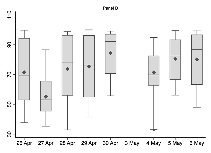
2

1         Introduction
The 2010 U.S. Flash Crash served as a sharp reminder of the potential fragility of
the international financial system. On 6 May 2010, around 2:30 in the afternoon,
U.S. equity markets started showing extraordinary large declines.1 Within minutes,
the Dow Jones had lost more than 6% of its value. For some individual securities,
the declines were even stronger, with some trades being executed at prices as low
as a penny. It was only after a brief trading halt at 2:45 p.m. that financial
markets recovered (CFTC-SEC, 2010). The Flash Crash also had large international
repercussions. In Canada, the equity index declined by more than 3% (IIROC, 2010).
On Latin American equity exchanges, prices of individual stocks declined by up to
10% (Jansen, 2018). The importance of understanding why this crash occurred
was further underlined by a number of subsequent flash events. For instance, U.S.
Treasury yields showed extraordinary volatility after market open on 15 October
2014; the British pound suddenly lost 6% against the U.S. dollar on 7 October 2016;
and the euro unexpectedly dropped by 3% against the dollar on Christmas Day
2017.
        Although finding a root cause for the 2010 Flash Crash proved difficult, a number
of contributing factors have been suggested. A joint staff report by the Commodity
Futures Trading Commission and the Securities and Exchange Commission iden-
tified the activation of a sell algorithm for E-Mini contracts — index futures con-
tracts based on the S&P 500 — as the immediate trigger for the crash (CFTC-SEC,
2010). From the E-Mini market, the crash then spilled over to the rest of the U.S.
financial system (see, e.g., Madhavan (2011), Kirilenko et al. (2017), or Menkveld
and Yueshen (2017)). Also, some papers have pointed to adverse developments in
order flow dynamics in the days before the crash (Easley, López de Prado, and
O’Hara, 2011, 2012).2 Furthermore, U.S. authorities prosecuted a London-based
trader who, in 2016, pleaded guilty to repeated attempts of trying to manipulate
the market for E-Mini contracts (Department of Justice, 2016).
    1
        Times in this paper are, unless indicated otherwise, denoted in Eastern Daylight Time (EDT).
    2
        Their measure for order flow toxicity has, however, been the subject of some debate. See
Andersen and Bondarenko (2014) and Easley et al. (2014).
3
This paper contributes to the literature on the origins of the flash events by
studying the possible role of spillovers from Europe to the U.S. in the hours before
the 2010 Flash Crash. As observers already noted at the time, the European trading
session on 6 May had been an extremely nervous one.3 First and foremost, financial
markets were closely following social and political developments in Greece, where the
lingering sovereign debt crisis was reaching a crucial stage. On 2 May, the Interna-
tional Monetary Fund and the European Union had reached an agreement with the
Greek government on a e110 billion financial support package. However, this agree-
ment required Greece to make rigorous adjustments to its government finances.4
These adjustments, such as reductions in government wages and pensions, had led
to severe social unrest. On 6 May, the Greek parliament was scheduled to debate
the fiscal adjustment measures, with a crucial vote being expected sometime during
the evening in Greece. That same day, there would also be fierce debates in the
German parliament, which was divided regarding Germany’s sizeable contribution
to the financial support package.
A second reason why European markets were nervous was a growing fear of
contagion from the Greek sovereign debt crisis to the rest of Europe. Primarily,
markets worried about high levels of government debt in Spain, Italy, Portugal, and
Ireland. Spreads on credit default swaps for these countries’ government debt had
been widening considerably. In addition, markets were nervous about the strength
of banking sectors in these countries, given the large exposures to their home coun-
tries’ government debt. More broadly, market participants started thinking about
contagion to the banking sectors of other European countries. For instance, various
French financial institutions came under scrutiny for their exposures to Greek gov-
ernment debt. A ratings report by Moody’s, released during the European morning
trading session of 6 May, suggested that sovereign risk contagion could also affect
the U.K. banking sector.
3
These descriptive paragraphs build on CFTC-SEC (2010) and news reports by CNN (Twin,
2010), the Financial Times, (Nolan, 2010), the Guardian (Roberts, 2010), the New York Times
(Bowley, 2010), and the Wall Street Journal (Lauricella and McKay, 2010).
4
For details, see https://www.imf.org/en/News/Articles/2015/09/28/04/53/
socar050210a, URL last accessed on 19 October 2018.4 A third factor driving market sentiment on 6 May was the upcoming mone- tary policy decision by the European Central Bank. The ECB’s Governing Council was meeting in Lisbon that day, and the ECB would announce its latest monetary policy decision at 13:45 CEST (07:45 EDT). Markets were especially interested in ECB President Trichet’s remarks at the subsequent press conference. There was some speculation that the ECB would end up buying government bonds to contain the sovereign debt crisis. However, at the press conference, Trichet immediately indicated that such a step had not even been discussed. Overall, market reactions to the ECB decisions were negative, as investors were disappointed with what was seen as complacency by the ECB. A final factor adding to the news flow on 6 May was the general election in the United Kingdom. Prime Minister Gordon Brown had called for this election in early-April. Various polls were indicating that it would be a close contest between Brown’s Labour Party and the Conservatives led by David Cameron. In the end, neither party was able to win an absolute majority. Throughout the day, however, the market reaction to election news was muted, and dynamics in U.K. equity prices were primarily driven by news on the sovereign debt crisis. Given the intense news flow and the predominantly negative sentiment in the European trading session, there is good reason to study spillovers from Europe to the U.S. in the hours before the Flash Crash. To do so, this paper uses the approach proposed by Diebold and Yilmaz (2009). Their idea is to start by estimating vector autoregressive models, before subsequently running forecast-error variance decom- positions to measure spillovers. Such an approach is especially useful when the key issue is not necessarily to determine whether any spillovers are due to interdepen- dence or contagion (cf. Forbes and Rigobon, 2002). To estimate spillovers, this paper uses minute-by-minute data on stock market indices in Europe and the U.S. In terms of research design, the paper compares intraday spillovers, both for returns and volatility, on 6 May with those during the preceding two weeks of market trad- ing. These intraday spillovers can be estimated by making use of the two-hour time window during which U.S. and European trading hours overlap each business day.
5

    This paper concludes that spillovers from European stock markets to the U.S.
did not increase in the hours before the 2010 Flash Crash. During the two-hour time
window on 6 May where European and U.S. trading overlapped, spillovers to the
U.S. were at levels comparable to, or lower than, those in the preceding two weeks of
stock-market trading. This conclusion holds for return as well as volatility spillovers,
and it is robust across a range of VAR models that were considered to capture
various dynamics in the news flow in Europe on 6 May. Overall, these findings
underscore the difficulties in understanding the nature of flash events in financial
markets. Though perhaps intuitively appealing, a narrative based on spillovers from
the European debt crisis seems to offer little guidance for a deeper understanding
of the flash events in financial markets.

2     Research Design
To study spillovers, this paper uses the approach proposed by Diebold and Yilmaz
(2009). The literature has since long studied how shocks can spill over via inter-
national financial markets. Various approaches are available, for instance the ana-
lysis of cross-market correlations (King and Wadhwani, 1990), the use of (G)ARCH
frameworks (Lin et al., 1994), and the study of factor models (Bekaert et al.,
2014). In many types of analysis, an important question is whether any evidence
for spillovers should be attributed to interdependence or contagion. As first stressed
by Forbes and Rigobon (2002), contagion only occurs when reactions to shocks are
in excess of normal cross-market comovements. For the present paper, however,
this distinction between interdependence and contagion is less important. Merely,
the aim is to see whether shocks in European markets had a greater effect on U.S.
markets in the hours immediately prior to the 2010 Flash Crash. The method by
Diebold and Yilmaz offers a straightforward route to answering this question.
    Computing Diebold-Yilmaz spillover indices requires taking the following three
steps. First, one estimates a vector autoregressive (VAR) model, where the endoge-
nous variables can be either returns or measures for asset price volatility. Second,
based on the VAR model, a variance decomposition for forecast errors (FEVD) is
6
calculated. In the third step, the spillover index is computed based on the FEVD
results. The crucial point is using the FEVD to distinguish between own-variance
shares and cross-variance shares. For measuring spillovers, only the cross-variance
shares are relevant. These shares measure the contribution to the n-step ahead
forecast-error variance in forecasting xi due to shocks in xj , where i 6= j (Diebold
and Yilmaz, 2009; Diebold and Yilmaz, 2010). The total spillover is the sum of all
cross-variance shares. This sum of cross-variance shares is then scaled by the sum
of relative contributions to the forecast-error variance. This scaling results in an
index that lies between 0 and 100, where 100 would indicate that the forecast-error
variance is completely due to cross-variance shares, i.e. spillovers.
At this point, it is important to note that the empirical results of this paper
will not center on the standard Diebold-Yilmaz indicator, i.e. the sum of all cross-
variance shares divided by the number of variables (Diebold and Yilmaz, 2010).
Rather, this paper focuses on a specific sub-set of the cross-variance shares, namely
those that measure the contribution of innovations in European returns to the
forecast-error variance of U.S. returns. This measure, which also ranges between
0 and 100, is more directly suited for answering the main research question of this
paper, namely whether spillovers from Europe were larger in the hours before the
Flash Crash. For comparison, however, an extension in Section 5 will discuss results
for standard Diebold-Yilmaz indices using all cross-variance shares.
The estimations in this paper use minute-by-minute data for stock market in-
dices in the U.S. and six European countries. The data source is Bloomberg. For
European indices, the data set includes observations for Spain (the IBEX 35), Italy
(the DJ Titans 30), Portugal (the PSI 20), Greece (the FT/ASE), Germany (the
DAX), and the U.K. (the FTSE 100).5 For the U.S., the paper uses the Dow Jones
Industrial Average. The stock index data covers the nine trading days in the period
from Monday 26 April to Thursday 6 May 2010. To estimate the VAR models, we
transform the levels of the stock market indices to minute-by-minute returns by tak-
5
This paper has no intraday stock market data for Ireland available. The assumption is that
the dynamics concerning possible contagion are captured by including the four Southern-European
economies.7
ing percentage differences. To study volatility, we use squared index returns, again
on a minute-by-minute basis.6
To measure intraday spillovers, this paper makes use of the partial overlap be-
tween trading hours in the U.S. and Europe. U.S. markets open at 9:30, which
corresponds to 14:30 in the U.K. and 15:30 in most of continental Europe. There-
fore, at the end of the each European trading session, there is generally a two-hour
window with simultaneous trading at the local stock exchange and in U.S. markets.
For any of the nine days in the sample, we can thus estimate a VAR model using
120 minute-by-minute observations. Using these VAR models, we can then calculate
the level of spillovers between Europe and the U.S. on any particular trading day.
To put dynamics on the day of the Flash Crash in perspective, we can compare the
level of spillovers during the last two hours of the European trading session on 6
May to the levels during this time slot on each of the preceding eight business days
in the sample.
The analysis is, admittedly, subject to a number of caveats. The most fundamen-
tal caveat is that the period with simultaneous trading on 6 May does not include
the Flash Crash episode itself. As European equity markets had all closed at 11:30,
there is a three-hour gap separating the analysis of this paper from the start of
the Flash-Crash episode. Any potential evidence of spillovers should, therefore, not
necessarily be seen as evidence for a causal chain of events. However, a larger degree
of spillovers on the morning of 6 May would corroborate the notion that negative
sentiment from Europe contributed to a market environment in which a flash event
could materialise.
Second, it should be remembered that the daily VAR models rely on, at most, a
two-hour window. Therefore, 120 minute-by-minute observations are available per
trading day, which only leaves sufficient degrees of freedom when the number of
lags p and the number of endogenous variables k remain sufficiently small.7 As a
result, the research design cannot readily analyse larger systems with richer types of
6
Diebold and Yilmaz (2009) measure volatility using open/high/low/close prices, which are,
unfortunately, not available for this paper.
7
The number of estimated parameters for a VAR model equals k + pk 2 . For a 5-variable VAR
with two lags, this means already the estimation of 55 parameters.8 lag specifications. For the baseline results, we consider models with two lags. The robustness analysis in Section 5 will show that the conclusions are robust to using richer lag structures in bivariate VAR systems. A third complication concerns data availability for Greece and Portugal. The reason for these limitations differs across the two countries. For Greece, the addi- tional time difference of one hour with the U.S. restricts the number of data points per day. Financial markets in Greece close at 17:20, which corresponds to 10:20 in the U.S. This means the number of observations with trading overlap is only 50 per day. For Portugal, some observations are, unfortunately, missing in the data feed. This means the sample with overlap in trading on that day only starts at 10:00 in- stead of 9:30. We address these two data challenges by never including both Greece and Portugal in the same VAR model. This paper estimates VAR models for seven distinct combinations of countries. All of the VAR models include, of course, U.S. data. The models differ, however, in their use of European market data. Firstly, by varying the set of countries in the model, we take into account the various dimensions of the news flow in Europe on 6 May. Secondly, using different sets of countries helps in addressing, as much as possible, the data gaps for Greece and Portugal. For all VAR models, rather than showing the Diebold-Yilmaz (2009) spillover index itself, the paper reports the contributions of European cross-variance shares to the forecast errors for the U.S. stock market. This measure gives the most direct answer to the research question. We start with four models that focus on the separate elements of news flow on 6 May 2010. The first model is a bivariate VAR that uses stock index returns (or volatility) for the U.S. and Greece. In terms of news flow, this model focuses on the key element driving market sentiment on 6 May, namely the debate in the Greek parliament on the EU-IMF financial assistance package. However, in terms of data, this model relies on the smallest number of observations. A second VAR model focuses on the possible contagion to other highly-indebted economies by estimating a system that includes data for the U.S., Spain, Italy, and Portugal. The third model is a bivariate VAR that uses data for the U.S. and Germany. Being the largest euro area economy, using Germany proxies for reactions to the ECB monetary-policy
9

decision on 6 May. It also directly captures potential reactions to the debates in the
German parliament on 6 May. A fourth model is a VAR system for the U.S. and the
U.K. This model captures market reactions to the U.K. general election and worries
about contagion of the sovereign debt crisis to the U.K. banking sector.
        The remaining three models combine the four elements of the news flow on
6 May. First, we estimate a VAR model that includes two Southern-European
economies (namely Spain and Italy), the U.K., and Germany. In two subsequent
models, we add data for either Portugal or Greece, in light of the data gaps for
these two countries. In terms of factorisation for the Cholesky decomposition, the
U.S. is always placed first, followed by, respectively, the U.K., Germany, and the
Southern-European countries. Section 5 will show that the Cholesky ordering does
not fundamentally change the conclusions on spillovers from Europe to the U.S.

3         Descriptives
We start by charting equity-market dynamics in Europe on 6 May. To that end,
Figure 1 shows scaled levels of stock market indices. The horizontal axis represents
hours according to Eastern Daylight Time. Indices are scaled so that levels at the
open of the U.S. market at 9:30 EDT (or 15:30 CEST) equal 100. The solid black
lines represent the FT/ASE 20 (Greece), the IBEX 35 (Spain), the Dow Jones Italy
Titans 30 (Italy), the PSI 20 (Portugal), the DAX (Germany), and the FTSE 100
(England). The gray dotted line in each panel denotes the scaled level of the Dow
Jones Industrial Average between 9:30 and 14:45 EDT.8

        insert Figure 1 here

During the European trading session on 6 May, there were three distinct patterns
in stock-market dynamics. Firstly, in Greece, markets showed particularly large
upswings as well as downswings (Figure 1, top-left panel). Greek stock trading
    8
        As noted, for Portugal, observations between 06:30 and 10:00 EDT are missing from the data
feed.
10 opened positively, but showed a sharp downward correction between 5:20 and 5:45 EDT. Sentiment then quickly turned positive again, but only until a second sharp correction shortly before 9:00, presumably as a reaction to the news from the on- going ECB’s monetary-policy press conference in Lisbon. Over the whole trading day, Greek stocks posted small gains, perhaps reflecting the growing belief that the Greek parliament would support the agreement on financial assistance with the IMF and the EU. Secondly, in the three other Southern-European countries, markets initially posted small gains. This upward trend ended around the time that markets in Greece showed the first sharp downward correction. From that point onwards, stock prices in Spain, Italy, and Portugal continuously declined. Initially, these three markets still moved more or less in line with U.S. markets. However, after 10:00 markets in Southern Europe started posting large declines. For instance, the Italian equity market lost around 3.5% of its value between 10:00 and market close at 11:30. Thirdly, for most of the trading session, volatility was low in Germany and the U.K. Markets were trending sideways, with indices remaining close to the levels at which equity markets had opened. It was not until the end of the European trading session that German and U.K. markets increasingly started to show losses. This decline came on the back of the ECB’s press conference and the sharp fall in Southern-European equities. On the whole, equities in Germany posted a small loss (of 0.2%) during the trading day, while stocks in the U.K. posted a small gain (of 0.2%). Turning to summary statistics, Table 1 gives an overview of means and standard deviations for index returns and squared returns. The table summarizes data for six European countries and the U.S. These statistics relate to the nine business days in the sample, i.e. the time span between Monday 26 April and Thursday 6 May 2010. The sample includes, for each of these nine days, the time window of roughly two hours where European and U.S. trading hours overlap. These observations form the basis for the estimation of the vector autoregressive models. In terms of mean returns, the Greek equity market is, in fact, the only one that posted gains over this two-week period. Average returns per minute are 0.005% for the FT/ASE index
11

(Table 1, column 1). The largest losses are for Italy, and Portugal, both of whom
lost on average 0.006% per minute during the sample period. In terms of volatility,
squared returns were, on average, largest in Southern Europe (Table 1, column 3).
In Greece, squared returns averaged 0.015%. In Spain and Italy, the averages for
squared returns were, respectively, 0.012% and 0.009%.

    insert Table 1 here

4     Baseline results for spillovers
Starting with equity returns, Figures 2 and 3 present baseline spillover results, es-
timated for each business day between 26 April and 6 May. Each daily sample
uses the two-hour window where trading in the U.S. overlaps with European market
hours. This means that every data point in Figures 2 and 3 refers to a value for
a spillover index, computed on the basis of a vector autoregressive model for that
particular business day. The y-axis in the two figures shows the percentage contri-
bution of shocks originating in European stock markets to forecast-error variances
for U.S returns. The underlying vector autoregressive models are of order 2 and
use minute-by-minute index returns. The ordering for the Cholesky factorisation is
shown in the legend of the figures. The forecast errors use a ten-minute horizon.
Figure 2 shows results for the four models that capture the individual pieces of news
flow on 6 May. Panel A focuses on news dynamics in Southern Europe. Panel B
focuses on the interactions between U.S. markets and either Germany or the U.K.
Figure 3 summarizes spillovers according to three additional VAR models that com-
bine the news-flow elements. The first model uses stock index returns in the U.S.
and five European countries. The second and third model add, respectively, index
returns in Portugal or Greece.

    insert Figures 2 and 3 here

Most importantly, and to some extent already answering this paper’s research ques-
12 tion, Figures 2 and 3 indicate no clear increase in return spillovers from Europe to the U.S. on the morning of 6 May, the day of the Flash Crash. For the four VAR models summarized in Figure 2, the spillovers from Europe on 6 May are never more than 5%. In fact, for three of the four models, the spillover index on that day is less than 1%. In other words, according to these estimates, around 99% of the forecast error variance for U.S. returns came from the U.S. The spillovers on 6 May were mostly comparable to or, in some cases, smaller than those on the preceding three trading days. The degree of spillovers in the week of the Flash Crash was, in fact, comparatively limited. This point follows from comparing the left part of the two panels in Figure 2, which report results for the trading week of 26 April, with the right-hand side of each panel. In both weeks, spillovers from Europe to the U.S. were small, as less than 10% of the forecast-error variance came from innovations in European returns. However, in the week preceding the Flash Crash, spillovers were distinctly larger. For instance, spillovers were relatively high on 28 April (around 5% for the model with Greece in Panel A) and 30 April (more than 5% for the model with Germany in Panel B). Overall, these patterns may suggest that the IMF-EU financial support package had something of a calming effect on financial markets in the week of 3 May 2010. The three VAR models that combine news-flow elements also indicate no increase in spillovers on 6 May. Figure 3 reports the results. The patterns across the two trading weeks generally echo those reported in Figure 2. Firstly, spillovers were higher in the week of 26 April compared to the week after the agreement between the Greek government and the IMF and EU. Second, spillovers were high on 28 April and 30th April, ranging between 30% on the latter and 50% on the former day. Third, there is no clear increase in spillovers in the hours before the crash on 6 May. In fact, based on these three VAR models, the level of spillovers on that day is the lowest of the nine daily estimates in this sample period. Turning to volatility spillovers, Figures 4 and 5 report results based on models for squared returns. The two panels in Figure 4 focus on the four individual news factors, while Figure 5 reports results for three VAR models with larger sets of en-
13
dogenous variables.
insert Figures 4 and 5 here
Figure 4 reinforces the point that spillovers were larger in the week of 26 April
compared to the week of the Flash Crash. For the bivariate model that includes
the U.S. and Greece, volatility spillovers are estimated to have been especially large
on 27 and 29 April (Figure 4, panel A). For the other three models in Figure 4,
the spillovers are relatively large on Friday 30 April. For instance, on the basis of
the model for U.S. and German returns, volatility spillovers are estimated to have
been more than 30% on that day. Compared to these levels of spillovers, the week
of 3 May was relatively tranquil. For the hours before the crash on 6 May, all four
models indicate that volatility spillovers were, at most, 5%.
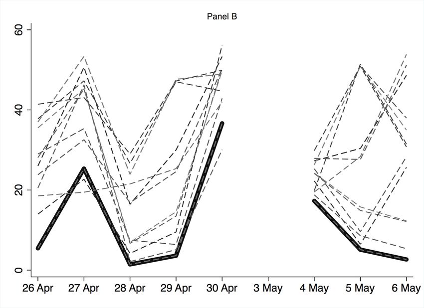
Finally, the results reported in Figure 5 are in line with the conclusions so far. All
three VAR models point to relatively large volatility spillovers on 30 April. These
spillovers are, in two cases, around 40%. For the model that includes Greece, the
sum of cross-variance shares is close to 50%. For the week of 3 May, spillovers are
generally smaller. For the model that includes Greek returns, the spillovers are
largest, and these lie around 20%. For the other two VAR models, the spillovers
actually decline in the course of the week of the Flash Crash.
5 Robustness and extension
This section starts with discussing two robustness checks concerning the specification
of the vector autoregressive models. An extension discusses Diebold-Yilmaz (2009)
indices based on all cross-variance shares.
First, we show that the conclusions do not change materially once we consider
alternative orderings for the Cholesky decomposition. Here, we focus on the VAR
model that combines the four elements of news flow with the highest number of avail-
able observations, i.e. the 5-variable VAR denoted by the black lines in Figures 4
and 5. In principle, given the sheer size and importance of U.S. financial markets, it14 seems most logical to focus on models that order U.S. returns first. In fact, Diebold and Yilmaz (2009) also use such an ordering in their baseline estimations. However, for a 5-variable VAR, it still possible to study all possible orderings, which is why we report results for 120 different forecast-error variance decompositions. It should be noted that, at some point, alternative strategies are needed, as the dimensions of the VAR system increase with the factorial of the number of variables (Diebold and Yilmaz, 2009; Klößner and Wagner, 2014). Figures 6 and 7 describe the results for these 120 different orderings, where Figure 6 focuses on the 24 models that order the U.S. first, and Figure 7 shows boxplots for the 96 models that do not order the U.S. first. In both figures, the top panel focuses on return spillovers, while the bottom panel reports results for volatility spillovers. In the top panels of Figures 6 and 7, the solid black lines corresponds to the results for the baseline model, i.e. the model that uses the ordering U.S., U.K., Germany, Spain, and Italy. insert Figures 6 and 7 here Starting with models that order the U.S. first, we confirm the baseline finding that return spillovers from Europe to the U.S. on 6 May were limited (Figure 6, panel A). The 23 alternative orderings also indicate that return spillovers on the morning of the Flash Crash were lower than on the preceding eight trading days. Compared to the baseline model, spillovers are generally higher when using any of the other 23 permutations. In these alternative specifications, spillovers now reach levels of 20% - 25%. Turning to volatility, there are again no clear indications that spillovers on 6 May were exceptional, although these spillovers are no longer always estimated to have been lower than during the preceding few trading days (Figure 6, panel B). Spillovers according to the baseline model are among the lowest of the 24 possible models. In particular during the trading week of 26 April, volatility spillovers now often reach levels of 50% - 60%. Most alternative models confirm the relatively high levels of spillovers indicated by the baseline model for 27 and 30 April. For the trading week of 3 May, there is some heterogeneity across models. There are a few
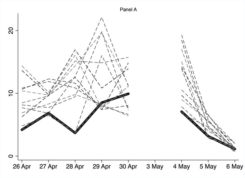
15

variants suggesting that spillovers increased from around 20% to 50% in that week,
but these latter levels are still comparable to those seen for the preceding trading
week.
   For decompositions that do not order the U.S. first, we generally find that
spillovers on 6 May were comparable to those in the preceding days. The two box
plots in Figure 7 show distributions for the 96 different orderings, where the boxes
indicate the 25th percentile, the median, and the 75th percentile. The diamonds
indicate sample means, and the dark circles show outliers. Starting with returns,
the average levels of spillovers (Panel A) are generally higher than those reported
in Figure 6. Given the different positioning of the U.S. in these decompositions,
this finding is not surprising. On average, daily return spillovers range between 70%
(for 27 April) and 85% (for 28 April). Average spillovers for 6 May lie towards
the top end of this range, but it should also be noted that there are several order-
ings (as indicated by the outliers) where the spillovers are only between 55% and
65%. For volatility, spillovers for 6 May are around 80% on average, which is a level
comparable to that on 5 May and 30 April.
   Second, we show that the baseline findings are robust to using richer lag specifi-
cations. Given that we can use, at most, 120 observations, the focus is on bivariate
models, as otherwise the number of estimated parameters would become too large.
We focus on five models that always include the U.S. and then add data from either
the U.K., Germany, Spain, Italy, or Greece. For these bivariate models, we consider
specifications with lag lengths of up to 5 and 10 minutes. Figure 8 reports the
results, once again measured as the contribution of European shocks to the forecast-
error variance for the U.S. The two top panels focus on return spillovers, while the
bottom panels focus on volatility spillovers.

   insert Figure 8 here

The main insight from Figure 8 is, once again, that spillovers on 6 May were not
exceptionally large. In most cases, spillovers were again larger in the week preceding
the Flash Crash. Having said that, the bivariate models for U.S. and Greece are an
16

important exception to this latter point. Return spillovers and volatility spillovers
now increase during the trading week of 3 May. This finding contrast the baseline
findings in Figure 3 and 4. Overall, though, spillovers on 6 May are still estimated
to have been lower compared to, say, those on 28 April (Figure 8, top left panel) or
29 April (bottom two panels).
        An extension reports Diebold-Yilmaz (2009) spillover indices that use all cross-
variance shares. Figure 9 reports these indices for three of the seven baseline models.
Panel A focuses on returns, and panel B reports spillovers for volatility.9 Again, we
conclude that spillovers on 6 May were not exceptionally large. For instance, for the
model that includes the U.S., the U.K., Germany, Spain, and Italy, return spillovers
are constant around a level of 60% during the sample period (Figure 9, panel A).
The exception is the bivariate model for the U.S. and Greece, where the spillovers
do increase to a level of around 15% in the course of the trading week of 3 May. For
volatility spillovers, such an upward trend is not observed.

        insert Figure 9 here

6         Conclusions
This paper finds no clear indications that spillovers from Europe contributed to
the 2010 Flash Crash in the U.S. financial system. Most importantly, we find no
robust evidence that equity-market spillovers were larger during the two-hour time
window on 6 May when European and U.S. stock-market trading overlapped. On the
contrary, both return spillovers and volatility spillovers were at levels comparable to,
or much lower than, those in the preceding few trading days. This finding is based
on the Diebold-Yilmaz (2009) approach that uses vector autoregressive models to
measure spillovers. The conclusion is robust across a range of VAR models that
capture various elements of the news flow in Europe on 6 May.
        When contrasted with the tumultuous news flow stemming from Europe on 6
May 2010, this paper’s main conclusion may come as a surprise. At the time,
    9
        Results for the additional five models lead to similar conclusions; results available upon request.
17 it was widely noted that the European trading session was a nervous one, and the intraday stock-market data discussed in this paper indeed corroborates the view that sentiment was negative, especially on Southern-European equity markets. However, this paper helps putting the events of 6 May in perspective. The trading session may have been a nervous one, but to some extent nerves of market participants seemed to have calmed compared to the preceding days. Two elements seem relevant here. First, markets seem to have taken some reassurance from the agreement on financial assistance between the Greek government, the EU, and the IMF. Secondly, on 6 May itself, it became increasingly clear that the Greek parliament would support this agreement, and in the end, Greek stock markets did not post large losses on that day. If spillovers from Europe could have contributed to the materialization of flash events, it is perhaps more surprising that this did not already occur on any of the preceding few trading days, when the levels of spillovers to the U.S. were much higher. This paper’s results further underscore the difficulties in understanding the na- ture of flash events in financial markets. Very few, if any, commentators have actu- ally argued that negative sentiment surrounding the Greek debt crisis in itself caused the Flash Crash. However, pointing to the high levels of volatility in European mar- kets on 6 May has been an often-used narrative to, at the very least, provide some intuition for the occurrence of this major flash event. This paper suggests that this particular narrative should offer little guidance in future discussions on flash events. As an alternative, it seems more promising to keep studying the role of microstruc- tural factors, such as liquidity (Noss et al., 2017), order flow (Easley et al., 2011), or high-frequency trading (Kirilenko et al., 2017).
18

References
Andersen, Torben, and Oleg Bondarenko (2014).         ‘VPIN and the flash crash.’
Journal of Financial Markets 17(C): 1-46.
   Bekaert, Geert, Michael Ehrmann, Marcel Fratzscher, and Arnaud Mehl (2014).
‘The Global Crisis and Equity Market Contagion.’ Journal of Finance 69: 2597-
2649.
   Bowley, Graham (2010). ‘US Markets Plunge, Then Stage a Rebound.’ New
York Times, 6 May 2010. Available at https://www.nytimes.com/2010/05/07/
business/07markets.html, URL last accessed on 19 October 2018.
   CFTC-SEC (2010). ‘Findings regarding the market events of May 6, 2010.’
Report of the staffs of the CFTC and the SEC to the Joint Advisory Committee on
Emerging Regulatory Issues. Released on 30 September 2010.
   Department of Justice (2016). ‘Futures Trader Pleads Guilty to Illegally Manip-
ulating the Futures Market in Connection With 2010 “Flash Crash” ’. Press release,
9 November 2016.
   Diebold, Francis X., and Kamil Yilmaz (2009). ‘Measuring Financial Asset Re-
turn and Volatility Spillovers, with Application to Global Equity Markets.’ Economic
Journal 119(534): 158-171.
   Diebold, Francis X., and Kamil Yilmaz (2010). ‘Erratum to: Measuring Financial
Asset Return and Volatility Spillovers, with Application to Global Equity Markets.’
Economic Journal 120(August): F354.
   Easley, David, Marcos M. López de Prado, and Maureen O’Hara (2011). ‘The
Microstructure of the ‘Flash Crash’: Flow Toxicity, Liquidity Crashes and the Pro-
bability of Informed Trading.’ Journal of Portfolio Management 37(2): 118-128.
   Easley, David, Marcos M. López de Prado, and Maureen O’Hara (2012). ‘Flow
Toxicity and Liquidity in a High-Frequency World.’ Review of Financial Studies
25(5): 1457-1493.
   Easley, David, Marcos M. López de Prado, and Maureen O’Hara (2014). ‘VPIN
and the Flash Crash: A rejoinder.’ Journal of Financial Markets 17(C): 47-52.
19

   Forbes, Kristin J., and Roberto Rigobon (2002). ‘No Contagion, Only Interde-
pendence: Measuring Stock Market Comovements.’ Journal of Finance 57: 2223-
2261.
   Jansen, David-Jan (2018). ‘The international spillovers of the 2010 U.S. Flash
Crash.’ DNB Working Paper No. 589.
   King, Mervyn A., and Sushil Wadhwani (1990). ‘Transmission of Volatility be-
tween Stock Markets.’ Review of Financial Studies 3(1): 5-33.
   Kirilenko, Andrei A., Albert S. Kyle, Mehrdad Samadi, and Tugkan Tuzun
(2017). ‘The Flash Crash: High-Frequency Trading in an Electronic Market.’ Journal
of Finance 72(3): 967-998.
   Klößner, Stefan, and Sven Wagner (2014). ‘Exploring all VAR ordering for
calculating spillovers? Yes, we can! — A note on Diebold and Yilmaz (2009).’
Journal of Applied Econometrics 29: 172-179.
   Lauricella, Tom, and Peter A. McKay (2010). ‘Dow Takes a Harrowing 1,010.14-
Point Trip.’ Wall Street Journal, 6 May 2010.
   Lin, Wen-Ling, Robert F. Engle, and Takatoshi Ito (1994). ‘Do bulls and bears
move across borders? International transmission of stock returns and volatility.’
Review of Financial Studies 7(3): 507-538.
   Madhavan, Anath (2011). ‘Exchange-Traded Funds, Market Structure and the
Flash Crash.’ Available at http://papers.ssrn.com/sol3/papers.cfm?abstract_
id=1932925.
   Menkveld, Albert J., and Bart Z. Yueshen (2017). ‘The Flash Crash: A Caution-
ary Tale about Highly Fragmented Markets.’ Forthcoming at Management Science.
   Nolan, Gavan (2010). ‘CDS report: Its getting worse’ Financial Times Al-
phaville, 6 May 2010. Available at https://ftalphaville.ft.com/2010/05/06/
222286/cds-report-its-getting-worse/, URL last accessed on 19 October 2018.
   Noss, Joseph, Lucas Pedace, Ondrej Tobek, Oliver Linton, and Liam Crowley-
Reidy (2017). ‘The October 2016 sterling flash episode - when liquidity disappeared
from one of the worlds most liquid markets’. Bank of England Staff Working Paper
No. 687.
20

   Roberts, Dan (2010).   ‘Business blog eurozone crisis.’   On-line blog at the
Guardian, 6 and 7 May 2010. Available at https://www.theguardian.com/business/
blog/2010/may/06/eu-debt-crisis-greece-live-blog-ecb,
URL last accessed on 19 October 2018.
   Twin, Alexandra (2010). ‘Glitches send Dow on wild ride.’ CNN Money, 6
May 2010. Available at https://money.cnn.com/2010/05/06/markets/markets_
newyork/, URL last accessed on 19 October 2018.
21

              Greece                      Spain                      Italy
   102

                              102

                                                         102
   98

                              98

                                                         98
   94

                              94

                                                         94
         04       10     15         04      10      15         04      10      15

              Portugal                   Germany                    England
   102

                              102

                                                         102
   98

                              98

                                                         98
   94

                              94

                                                         94

         04       10     15         04      10      15         04      10      15

Figure 1. Equity Markets in Europe and the U.S. on 6 May 2010 The
panels show scaled levels of stock market indices in six European countries on 6
May 2010, the day of the flash crash in the U.S. financial system. The horizontal
axis represents hours according to Eastern Daylight Time (EDT). Indices are scaled
so that levels at the open of the U.S. market at 9:30 EDT equal 100. The solid black
lines represent the FT/ASE 20 (Greece), the IBEX 35 (Spain), the Dow Jones Italy
Titans 30 (Italy), the PSI 20 (Portugal), the DAX (Germany), and the FTSE 100
(England). The gray dotted line in each panel denotes the scaled level of the Dow
Jones Industrial Average between 9:30 and 14:45 EDT. For Portugal, observations
between 06:30 and 10:00 EDT are missing from the data feed.
22 Figure 2. Return Spillovers From Europe to the U.S. Based on four VAR models, the panels report return spillovers from Europe to the U.S. for nine daily samples between Monday 26 April and Thursday 6 May 2010. Each sample uses the two-hour window where trading in the U.S. overlaps with Europe. The y-axis show the percentage contribution of shocks originating in Europe to the forecast- error variance for U.S index returns, following Diebold-Yilmaz (2009). The panel legends indicate the Cholesky ordering. Forecast errors use a ten-minute horizon. U.K. markets were closed on 3 May.
23

Figure 3. Return Spillovers From Europe to the U.S. The three underlying
VAR models combine stock index returns for European markets with index returns
on the Dow Jones Industrial Average. U.K. markets were closed on 3 May. For
further details, see notes to Figure 2.
24

Figure 4. Volatility Spillovers From Europe to the U.S. See also notes to
Figure 2. In this case, the endogenous variables are squared index returns.
25

Figure 5. Volatility Spillovers From Europe to the U.S. See also notes to
Figure 2. In this case, the endogenous variables are squared index returns.
26

Figure 6. Spillovers for Decompositions Ranking U.S. First. This figure
shows spillovers from Europe to the U.S., based on 24 Cholesky decompositions that
order the U.S. first. The other countries included are the U.K., Germany, Spain,
and Italy. Panel A shows return spillovers, panel B shows volatility spillovers. The
black solid line in Panel A corresponds to the black line in Figure 3; the black line
in Panel B corresponds to that in Figure 5.
27

Figure 7. Spillovers for Decompositions Not Ranking U.S. First. The box
plots summarize the distribution of spillovers according to 96 Cholesky orderings,
all based a five-variable VAR, that do not rank the U.S. first. The other countries
in the vector autoregressive model are the U.K., Germany, Spain, and Italy. Panel
A shows return spillovers, panel B shows volatility spillovers. The lines in the boxes
denote the median, the 25th percentile, and the 75th percentile. The black diamonds
denote means, the dark circles outliers.
28

Figure 8.    Robustness to Richer Lag Structures. The four panels show
spillovers from five European countries to the U.S., based on bivariate vector
autoregressive models.    The y-axes show the percentage contribution of shocks
originating in the respective European country to forecast-error variance for U.S
index returns, following Diebold-Yilmaz (2009). The two top panels focus on return
spillovers; the bottom panels focus on volatility spillovers. The models include
either up to 5 lags (left two panels) or 10 lags (right two panels).
29

Figure 9. Spillovers Between U.S. and Europe for Selected Models. The
two panels report results for the standard Diebold-Yilmaz (2009) spillover index
based on all cross-variance shares in a forecast-error variance decomposition. The
three selected models also include U.S. data, which is always ordered first in the
Cholesky factorisations. Panel A focuses on return spillovers, while panel B focuses
on volatility spillovers.
30

Table 1. Summary Statistics for Returns and Volatility
This table shows descriptive statistics for stock market indicators in six European
countries and the U.S. Columns (1) and (2) summarize means and standard devi-
ations for minute-by-minute index returns in percentage terms. Columns (3) and
(4) summarize squared returns. The sample period corresponds to the overlap be-
tween European and U.S. trading hours, i.e. the time span between 9:30 EDT and
11:30 EDT. The sample includes the nine business days from Monday 26 April to
Thursday 6 May 2010.
                                   (1)        (2)        (3)        (4)
                                  Returns               Sq. returns
  Country           Index         Mean      St. dev.    Mean      St. dev.
  England           FTSE100       -0.003     0.061      0.004      0.011
  Germany           DAX           -0.002     0.073      0.005      0.018
  Greece            FT/ASE        0.005      0.123      0.015      0.044
  Italy             DJ IT30       -0.006     0.095      0.009      0.020
  Portugal          PSI 20        -0.006     0.069      0.005      0.011
  Spain             IBEX 30       -0.004     0.111      0.012      0.052
  United States     DJIA          -0.001     0.051      0.003      0.006
Previous DNB Working Papers in 2019 None
De Nederlandsche Bank N.V.
Postbus 98, 1000 AB Amsterdam
020 524 91 11
dnb.nl
You can also read