Modelling Sustainable International Tourism Demand to the Brazilian Amazon
←
→
Page content transcription
If your browser does not render page correctly, please read the page content below
Modelling Sustainable International Tourism Demand to the
                               Brazilian Amazon

                                 Jose Angelo Divino
                               Department of Economics
                             Catholic University of Brasilia

                                Michael McAleer
                        Department of Quantitative Economics
                         Complutense University of Madrid

Abstract
The Amazon rainforest is one of the world’s greatest natural wonders and holds great
importance and significance for the world’s environmental balance. Around 60% of the
Amazon rainforest is located in the Brazilian territory. The two biggest states of the
Amazon region are Amazonas (the upper Amazon) and Pará (the lower Amazon), which
together account for around 73% of the Brazilian Legal Amazon, and are the only states
that are serviced by international airports in Brazil’s North region. The purpose of this
paper is to model and forecast sustainable international tourism demand for the states of
Amazonas, Pará, and the aggregate of the two states. By sustainable tourism is meant a
distinctive type of tourism that has relatively low environmental and cultural impacts.
Economic progress brought about by illegal wood extraction and commercial
agriculture has destroyed large areas of the Amazon rainforest. The sustainable tourism
industry has the potential to contribute to the economic development of the Amazon
region without destroying the rainforest. The paper presents unit root tests for monthly
and annual data, estimates alternative time series models and conditional volatility
models of the shocks to international tourist arrivals, and provides forecasts for 2006
and 2007.

Key Words: Brazilian Amazon; International Tourism Demand; Time Series
Modelling; Conditional Volatility Models; Forecasting.

JEL: C22; C53; Q23.

                                           1
1. Introduction
The Amazon rainforest holds great importance and significance for the world’s
environmental balance. As an idea of its importance and monumental size, the various
rivers that comprise the Amazon basin account for around 20% of the total volume of
fresh water that flows into the various oceans of the world. In short, the rivers of the
Amazon region form the biggest hydrographic network anywhere on the planet.
Specifically, the Amazon River is by far the world’s biggest river in terms of fresh
water volume. In addition, the biodiversity in the Amazon region is one of the richest of
the world, with a considerable amount of fauna and flora that have been sighted by very
few indigenous tribes and scientists. Medical researchers have suggested that the flora
in the Amazon region can provide a cure in the years ahead for several diseases that
afflict humanity.
Rainforests are effectively dense jungles. They are the oldest living ecosystem
on Earth, covering about 6% of its surface and accounting for two-thirds of the world’s
species of animals and plants. The Amazon represents over one-half of the world’s
remaining rainforests, and comprises the largest and most species-rich tract of tropical
rainforest anywhere. There are temperate rainforests, that are found further north or
south from Ecuador, and tropical rainforests, that are found along the warm and rainy
climate of the Ecuador line. Tropical rainforests are known by their dense vegetation
that forms three different layers, containing giant trees with a height of 75 meters or
more in the upper layer. The soil of a rainforest is generally very poor due to the lack of
sunlight and the high humidity. This combination of lack of sunlight and high humidity
makes the soil especially fragile when the forest is destroyed, even entering into a
process of desertification in some areas.
2The total extension of the Amazon rainforest is about 7 million square
kilometers, and is distributed across nine South American countries, namely Bolivia,
Brazil, Colombia, Ecuador, Guyana, French Guiana, Peru, Suriname, and Venezuela.
Around 60% of the Amazon rainforest is located in the Brazilian territory,
corresponding to virtually the entire North region of the country, and is called the
Brazilian Amazon1. The remaining 40% of the Amazon rainforest is distributed across
the other eight countries that share the forest, with the largest part being in the eastern
part of Peru. Large portions of the three Guineas, namely Guyana, Suriname and French
Guiana, are covered by the Amazon rainforest.
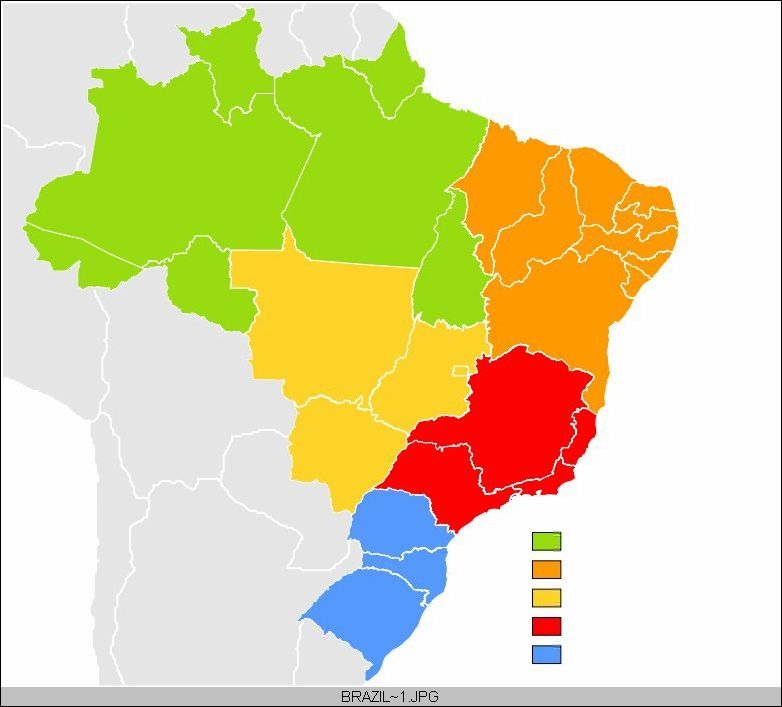
The 60% of the Amazon that is located in the Brazilian territory defines the so-
called Legal Amazon, and includes the states of Acre, Amazonas, Amapá, North of
Mato Grosso, Pará, Rondônia, Roraima, Tocantins, and West of Maranhão. Figure 1
presents a map of Brazil that emphasizes these states. Although Maranhão is actually a
state of the Brazilian Northeast region, it borders the east side of Pará state, which
means that its border on the West of Maranhão is covered by the Amazon forest, and
hence is a part of the Legal Amazon. The same holds for North of Mato Grosso, which
is a state of the Middle-East Region that borders South of Amazonas and Pará and West
of Rondonia. The two biggest states of the Amazon region are Amazonas (also referred
to as the upper Amazon) and Pará (also referred to as the lower Amazon), which
together account for around 73% of the Brazilian Legal Amazon.
Amazonas is the largest state of Brazil, with a total area of 1.6 million square
kilometres. This state is larger than any other country of the Amazon rainforest, and
virtually all of its area is occupied by rainforest or rivers. In addition to its size,
Amazonas state is surrounded by land, such that access to the region is by air or along
1
All the geographical data presented in this section has as source the official site of the Brazilian Institute
for Geography and Statistics (IBGE, Instituto Brasileiro de Geografia e Estatística), avalaible at
www.ibge.gov.br.
3the various rives that form the Amazon River and its tributaries. Large ships have access
to Amazonas from the Pará city of Belem, which is at the mouth of the Amazon River
where it flows into the Atlantic Ocean.
The capital of Amazonas state is Manaus, which is at the confluence of the two
main tributaries of the Amazon River, where the black water of the Rio Negro and the
yellowish brown water of the Rio Solimoes join to form the Amazon River. About 77%
of the Amazonas state forest remains intact, primarily due to the creation of the Free
Zone of Manaus (Zona Franca de Manaus) by the Brazilian Government in 1967 to
implement light industries in the region, mainly electronics and motorcycles. This
affirmative action has created job opportunities around Manaus and has contributed to
preserve the rainforest from being exploited for (possibly unsustainable) economic
activities. There have been significant efforts made by the Federal Government to
promote sustainable development in the region in order to preserve the natural
resources. The local economy is based on the light industrialization of the Free Zone of
Manaus, explorations for petrol and natural gas, fishing, mining, and natural
exploration. Several projects have recently been initiated in the region, including
technological innovation, biodiversity exploration, sustainable tourism, eco-tourism,
and education, all of which have been linked to widespread concerns about sustainable
economic development and growth.
The second largest Brazilian state is Pará, which has a total area of 1.2 million
square kilometers. Much of the Pará territory is also covered by the Amazon rainforest.
The discovery and extraction of latex from rubber trees was responsible for the
development of the state towards the end of the 19th century and beginning of the 20th
century. With the economic decline of natural latex and its replacement with synthetic
rubber, Pará experienced economic stagnation, which was overcome in around 1960s
4with the development of commercial agriculture and mineral exploration, mainly iron
and gold, in the south of the state.
As it might be expected, economic progress has been achieved at the cost of
destroying large areas of the Amazon rainforest. For example, there has been the
creation of an industrial zone around the metropolitan region of Belem, the Pará state
capital, and illegal extraction of wood from the Amazon forest. More recently,
widespread commercial agriculture and the bovine industry have moved toward the
southeast of the state, which has led to serious land conflicts and further destruction of
the Amazon rainforest.
In this scenario of destruction and illegal exploration of the rainforest, the
tourism industry would seem to have the potential to contribute to sustainable economic
development in the North region of Brazil. Activities linked to ecotourism, for instance,
would be a rational way of generating employment and income to the region without
causing damage to its abundant natural resources. However, tourism, especially
international tourism, is still in its infancy in the Amazon region. In this context, Figure
2 shows the distribution of tourism GDP, as computed for each Brazilian municipal
district by Divino et al. (2007). It is strikingly clear that tourism GDP is heavily
concentrated along the Northeast coastline and in the Southeast and South regions of the
country. In the North region, very few municipal districts show tourism GDP at the
upper level of the distribution, with much of the states of Amazonas and Pará having
very low tourism GDP. The sole exception to the low tourism GDP in the upper
Amazon rainforest is the Free Zone of Manaus. In general, tourism GDP in the upper
Amazon is extremely low, except in some cities and towns along the Amazon River and
its various tributaries.
5The primary purpose of this paper is to model and forecast sustainable
international tourism demand for the Brazilian Amazon. By sustainable tourism is
meant a distinctive type of tourism that has a lesser impact on the natural environment,
local communities and local cultures, as opposed to other economic activities that have
caused destruction of large areas of the rainforest. We will analyse international tourist
arrivals data for the two major states in the Amazon region, namely Amazonas and Pará,
which are the only states that are serviced by international airports in Brazil’s North
region. As mentioned previously, these two states account for around 73% of the
Brazilian Amazon, and are also the only two states in the Brazilian Amazon for which
monthly time series data over an extended period are available. In terms of the existent
literature, this paper may be seen as a precursor for future analyses of sustainable
tourism in the Brazilian Amazon region as there would seem to be no previous research
that has modelled and forecasted international tourist arrivals to the Brazilian Amazon
using reliable monthly time series data.
The development of a sustainable tourism industry would seem to be crucial for
the North region as it is presently the second poorest region in Brazil. Table 1 shows the
GDP and per capita GDP figures for each of the 27 Brazilian states and the 5 broad
regions. It shows that the per capita GDP of the North region is only US$1,509. Of the 7
states in the North region, marked in bold, 4 of them are among the 10 poorest states in
Brazil. Maranhão, which borders Pará state, is the poorest Brazilian state on the basis of
per capita GDP. Only the Amazonas state is among the top 10 states in Brazil. As
mentioned previously, the ranking of Amazonas state arises primarily because of the
Free Zone of Manaus that has generated employment and increased income through
light industrialization around the state’s capital, without destroying the Amazon
rainforest. It is envisaged that, with the development of sustainable exploration by local
6governments and private sector, international tourism can contribute significantly to the
sustainable economic development of the North region.
The tourism industry is still very underdeveloped in the Brazilian Amazon, but
has great potential for expansion. In 2007, for instance, the number of international
tourists arriving in Amazonas and Pará accounted for only 0.6% and 0.5%, respectively,
of the total number of international tourist arrivals to Brazil. Historically, within each of
these states, most of the tourist have come from the USA to Amazonas (51% in 2007)
and from French Guiana to Pará (46% in 2007). Other important sources of
international tourists are Canada and Venezuela to Amazonas and the USA and France
to Pará. Most of the international tourists come to these two regions because they
are attracted by ecotourism, followed by commerce in the free trade zone of Manaus,
and also for medical purposes. These two regions are not popular with domestic tourists,
with very few Brazilians travelling to the region.
There has recently been a growing literature that has applyied econometric
techniques to forecast tourism demand. Athanasopoulos et al (2009) provide
hierarchical forecasts for Australian domestic tourism demand, and produce detailed
forecasts of the Australian domestic tourism market. Bonham et al (2009) estimate a
fully identified vector error correction model of tourism for Hawaii, where both demand
and supply-side influences are important. They identify long run equilibrium
relationships and demonstrate satisfactory forecasting performance. Gil-Alana et al
(2009) apply different seasonal statistical models to forecast the numbers of tourists
travelling to the Canary Islands, Spain, and use different forecasting models for short
versus long run forecasts. Other important contributions to the tourism and
environmental forecasting literature include Ribbe et al. (2008), Anwar et al (2007), and
Ticehurst et al (2007). This paper contributes to the literature by modelling and
7forecasting international tourist arrivals to the Brazilian Amazon using reliable monthly
and annual time series data. It is the first paper that examines the usefulness of, such
models and provides forecasts of sustainable tourism demand for the Brazilian Amazon.
The structure of the remainder of the paper is as follows. Section 2 discusses the
monthly and annual international tourist arrivals to Amazonas, Pará and the total of the
two states. Section 3 presents unit root tests for the monthly and annual data to be
analysed. Alternative time series models for international tourist arrivals and conditional
volatility models are presented in Section 4, and their estimates are given in Section 5.
Forecasts of monthly and annual international tourist arrivals to Amazonas, Pará and the
total of the two states for 2006 and 2007 are given in Section 6. Some concluding
remarks are given in Section 7.
2. Data
The data set to be analysed consists of monthly time series data, as well as annual
aggregates, relating to international tourist arrivals for the two major states of the
Brazilian Amazon, namely Amazonas and Pará, for the period January 1971 to
December 2005. The sources of the data are the official reports of Embratur (Empresa
Brasileira de Turismo – Brazilian Enterprise of Tourism), which is an official branch of
the Federal Ministry of Tourism that is responsible for the compilation of tourism
statistics in Brazil. According to the Embratur statistical department, the numbers of
international tourist arrivals are computed from immigration cards that international
tourists are required to complete and submit to the Brazilian Federal Police before
entering the country. For the Brazilian Amazon, the immigration cards are tabulated
from the international airports in Manaus, the capital of Amazonas, and Belém, the
8capital of Pará. In addition to monthly data, we have also used annual data in
estimation and forecasting. The major advantages of using monthly data are to increase
the sample size from 35 annual observations to 420 monthly observations, and to
investigate the volatility that is inherent in the time series, which is a requirement for
estimating conditional volatility models accurately (for further details, see McAleer
(2005)). The annual tourist arrivals series correspond to the monthly aggregates for each
year. In the empirical analysis, we also consider the total number of international tourist
arrivals for Amazonas and Pará for both the monthly and annual time series, which are
obtained by adding the international tourist arrivals to the Amazonas and Pará states.
At the outset, it should be mentioned that there were nine missing observations
for the monthly series of international tourist arrivals for the Amazonas state in 1993.
According to Embratur, the missing monthly data arose from administrative problems at
the International Airport of Manaus. In order to obtain a complete and homogeneous
series of observations for both Amazonas and Pará, we estimated an ARMA model for
the monthly data to December 1992, then forecasted all 12 months of 1993, and used
the 3 months in 1993 for which there were observations to calibrate the accuracy of the
forecasts. Estimation of several alternative specifications with 12 seasonal dummy
variables suggested that the best fitting models were an unrestricted AR(2) model and
AR(12) model with zero restrictions for lags 3-11 inclusive. The Akaike Information
Criterion and Schwarz Bayesian Information Criterion slightly favoured the unrestricted
AR(2) model, but the aggregated forecasts for 1993 were very similar, namely 12,551
and 12,557, respectively. As the AR(12) term was only marginally significant at the 1%
level, but resulted in a loss of 10 observations, the unrestricted AR(2) model with 12
monthly seasonal dummy variables was used to forecast the monthly international
tourist arrivals to the Amazonas state for the 12 months of 1993.
9The calculation of missing monthly observations for Amazonas for 1993 leads to
the use of generated regressors for purposes of forecasting, with the associated critical
issues of generally inefficient estimation and invalid inferences that arise through the
use of biased (asymptotic) standard errors in the presence of sampling estimation errors.
Pagan (1984, 1986), Oxley and McAleer (1993, 1994), and McKenzie and McAleer
(1997) provide comprehensive discussions of these issues, including the impact of
generated regressors on obtaining forecasts and forecast standard errors.
The complete time series for monthly and annual international tourist arrivals are
displayed in Figures 3 and 4, respectively. These figures also show the respective
growth rates. From Figure 3, it is evident that there is an important seasonal component
but no deterministic trend component in the monthly series of international tourist
arrivals. As a result, the growth rates fluctuate around zero over time, with noticeable
volatility persistence in the monthly growth rates. In addition, the monthly time series
data are generally quite small numbers. For Amazonas, the monthly average of
international tourist arrivals was 1,093, with a maximum of 4,109 in January 1987 and
an amazing minimum of 2 in July 1991. For Pará, the situation is reasonably similar,
with a monthly average of 903 international tourist arrivals. However, the Pará time
series peaked in July 2005 with 4,394 international tourist arrivals, and with a minimum
of an extremely low 6 in October 1988. The monthly growth rates in international
tourist arrivals showed significant volatility, varying roughly between (-350%, 350%)
for Amazonas, (-400%, 500%) for Pará, and (-140%, 130%) for the total of the two
leading states.
On an annual basis for the period 1971-2005, the average number of
international tourist arrivals to Amazonas was 13,114, while this number was lower at
10,839 for Pará. From Figure 4, it is evident that there is no tendency for the growth in
10the number of international tourist arrivals to increase deterministically over time as the
annual growth rates have been close to zero for Amazonas, Pará and the sum of the two
states since 1971. The annual growth rates in international tourist arrivals were less
volatile than their monthly counterparts, and varied roughly between (-60%, 50%) for
Amazonas, (-90%, 90%) for Pará, and (-50%, 50%) for the total of the two leading
states.
The numbers of international tourists suggest that international tourism activity
has not been encouraged in the Brazilian rainforest. The Brazilian Amazon is one of the
richest geographic locations in the world for biodiversity, but the second poorest in
Brazil in terms of per capita income. Thus, the development of a sustainable tourism
industry should be able to preserve the rainforest and to generate substantial income for
the residents of the Amazon rainforest region.
3. Unit Root Tests
The first step in the modelling strategy was to test the time series for the existence of
one or more unit roots. A common criticism of traditional unit root tests, primarily those
based on the classic methods of Dickey and Fuller (1979, 1981) and Phillips and Perron
(1988), is that they suffer from low power and size distortions. However, these
shortcomings have been overcome by modifications to the testing procedures, such as
the methods proposed by Perron and Ng (1996), Elliott, Rothenberg and Stock (1996),
and Ng and Perron (2001).
For example, Elliott, Rothenberg and Stock (1996) demonstrate that OLS de-
trending is inefficient if the data presents high persistence, and suggest using GLS de-
trended data, which is efficient. Ng and Perron (2001) show that, in the presence of a
11strong negative moving average coefficient, the unit root estimate is strongly biased if
the lag truncation, k, is small because the residuals of the test equation are serially
correlated. In order to select the optimal value of k to account for the inverse non-linear
dependence between the bias in the unit root coefficient and the selected value of k, and
to avoid selecting an unnecessarily large value of k, Ng and Perron (2001) proposed a
modified Akaike Information Criterion (MAIC). Thus, the modified ADFGLS
(MADFGLS) test uses GLS de-trended data and the MAIC in order to choose the
truncation lag.
The modified Phillips-Perron test (MPPGLS), which also uses GLS de-trended
data and the MAIC to select the optimal truncation lag, is due to Phillips and Perron
(1988), Perron and Ng (1996) and Ng and Perron (2001). The asymptotic critical values
for both the MADFGLS and MPPGLS tests are given in Ng and Perron (2001).
The results of the unit root tests, which are obtained from the econometric
software package EViews 5.0 and reported in Table 2, indicate that the logarithm of
monthly international tourist arrivals for Amazonas (LAM) and the total of Amazonas
and Pará (LTO) have unit roots. For Pará (LPA), however, the tests indicate a stationary
time series. The annual data also indicate a stationary series for Pará. In the model with
just a constant as the deterministic term, however, the null hypothesis of a unit root is
rejected for Amazonas at the 5% level of significance. The aggregate of Amazonas and
Pará (LTO) is still non-stationary. Unit root tests were also applied to the monthly data
that were seasonally adjusted using the X11 method of the U.S. Census Bureau, but
there were no significant quantitative changes to the results.
In view of these empirical results, the first differences in the logarithms of
international tourist arrivals are used in estimating the models given below. This
transformation was deemed preferable as it would guarantee that all the time series are
12stationary and also provide the rate of growth of international tourist arrivals to
Amazonas, Pará, and the aggregate of the two states.
4. Conditional Mean and Conditional Volatility Models
The alternative time series models to be estimated for the conditional means of the
monthly and annual international tourist arrivals, as well as their conditional volatilities,
are discussed below. As Figure 3 illustrates, the growth rates of international tourist
arrivals to Amazonas, Pará and the total of the two states show periods of high volatility
followed by others of relatively low volatility. One implication of this behavior is that
the assumption of homoskedastic residuals is inappropriate. In this case, in order to
forecast the international tourist arrivals (or their growth rates, as appropriate), it is
necessary also to forecast their conditional variances.
Time-varying conditional variances can be explained empirically through the
autoregressive conditional heteroskedasticity (ARCH) model, which was proposed by
Engle (1982). When the time-varying conditional variance has autoregressive and
moving average components, this leads to the generalized ARCH(p,q), or GARCH(p,q),
model of Bollerslev (1986). The lag structure of the appropriate GARCH model can be
chosen by information criteria, such as those of Akaike and Schwarz, although it is very
common to impose a GARCH(1,1) specification in advance. In the selected conditional
volatility model, the residual series should follow a white noise process. Li et al. (2002)
provide an extensive review of recent theoretical results for univariate and multivariate
time series models with conditional volatility errors, and McAleer (2005) reviews a
wide range of univariate and multivariate, conditional and stochastic, models of
volatility.
13Consider the stationary AR(1)-GARCH(1,1) model for international tourist
arrivals (or their growth rates, as appropriate), y t :
yt = φ1 + φ2 yt −1 + ε t , φ2 < 1 (1)
for t = 1,..., n , where the shocks (or movements in international tourist arrivals) are
given by:
ε t = η t ht , η t ~ iid (0,1)
(2)
ht = ω + αε 2
t −1 + β ht −1 ,
and ω > 0, α ≥ 0, β ≥ 0 are sufficient conditions to ensure that the conditional variance
ht > 0 . The AR(1) model in equation (1) can easily be extended to univariate or
multivariate ARMA(p,q) processes (for further details, see Ling and McAleer (2003a)).
In equation (2), the ARCH (or α ) effect indicates the short run persistence of shocks,
while the GARCH (or β ) effect indicates the contribution of shocks to long run
persistence (namely, α + β ). The stationary AR(1)-GARCH(1,1) model can be
modified to incorporate a non-stationary ARMA(p,q) conditional mean and a stationary
GARCH(r,s) conditional variance, as in Ling and McAleer (2003b).
In equations (1) and (2), the parameters are typically estimated by the maximum
likelihood method to obtain Quasi-Maximum Likelihood Estimators (QMLE) in the
absence of normality of η t . The QMLE is efficient only if η t is normal, in which case it
is the MLE. When η t is not normal, adaptive estimation can be used to obtain efficient
14estimators. Ling and McAleer (2003b) investigate the properties of adaptive estimators
for univariate non-stationary ARMA models with GARCH(r,s) errors.
Ling and McAleer (2003a) showed that the QMLE for GARCH(p,q) is
consistent if the second moment of ε t is finite. For GARCH(p,q), Ling and Li (1997)
demonstrated that the local QMLE is asymptotically normal if the fourth moment of ε t
is finite, while Ling and McAleer (2003a) proved that the global QMLE is
asymptotically normal if the sixth moment of ε t is finite. Using results from Ling and
Li (1997) and Ling and McAleer (2002a, 2002b), the necessary and sufficient condition
for the existence of the second moment of ε t for GARCH(1,1) is α + β < 1 and, under
normality, the necessary and sufficient condition for the existence of the fourth moment
is (α + β ) 2 + 2α 2 < 1 . Extensions of several of these results for asymmetric conditional
volatility models are given in McAleer et al. (2007).
5. Estimates of Models
The empirical results for the estimated models, which are obtained using the
econometric software package package EViews 5.0, are reported in Table 3. For the
monthly growth rate of international tourist arrivals to Amazonas, all the estimated
coefficients are statistically significant at the 5% level. The AR(12) term was included
in the model to capture seasonal factors. The GARCH(1,1) coefficients indicate that the
persistence of shocks to Amazonas holds in both the short and long run, with the short
run persistence being quite small, though statistically significant. The AR(1) coefficient
of 0.41 implies that the growth rate of Amazonas is convergent. The diagnostic test,
provided by a Lagrange multiplier (LM) test for ARCH disturbances, indicates that
there is no need to include additional lags in the GARCH(1,1) specification. As the
15second and fourth moment restrictions, as given in Section 4, are satisfied for
Amazonas, the QMLE are consistent and asymptotically normal, so that standard
statistical inference is valid.
The estimated model for the monthly growth rate of international tourist arrivals
to Pará presented some coefficients that were not statistically significant. Specifically,
the constant and the GARCH(1) term were not statistically different at the 5% level.
The AR(1) coefficient was negative and close to zero, indicating a convergent process.
The GARCH(1,1) coefficients, however, suggest a very high persistence of shocks to
Pará in the short run, with the ARCH effect being 0.99, with the long run persistence
being quite small and insignificant at 0.07. The LM diagnostic test indicates that the
model is well specified for the selected GARCH terms.
The estimated model for the total of international tourist arrivals to the
Amazonas and Pará states shows that all the estimated coefficients, except for the
constant, are statistically significant. This time series is also convergent, given the
estimated AR(1) coefficient of 0.44, which is far inside the unit circle. The estimates of
the GARCH(1,1) model imply that the persistence of shocks decays very slowly for the
growth rate of the aggregate monthly data, with the short run persistence being small,
though statistically significant. The GARCH(1,1) coefficients indicate that the
persistence of shocks to Pará holds in both the short and long run, and the results for the
LM test suggest that the model is well specified. As for Amazonas, there is a strong
negative MA coefficient for the aggregated series. Moreover, the second and fourth
moment restrictions are satisfied for the aggregates series, as for Amazonas, so the
QMLE are consistent and asymptotically normal, so that standard statistical inference is
valid.
16For the annual data, it is interesting to note that there are no GARCH effects for
any of the three time series. This is in accordance with Figure 4, where the annual
growth rates of international tourist arrivals show a reasonably constant variance
throughout much of the sample period. The LM tests for the estimated ARMA models
indicate that there is no ARCH(1) or ARCH(2) effects in the estimated residuals. Thus,
the conditional variance of the residuals is constant over the period. In addition, the
estimated AR(1) coefficients are inside the unit circle, implying that the annual growth
rates are convergent.
6. Forecasts of Monthly and Annual International Tourist Arrivals
The previous models were used to forecast international tourist arrivals for Amazonas,
Pará, and the aggregate of the two states at both the monthly and annual frequencies for
the years 2006 and 2007. The results along with observed data for 2006 are presented in
Table 4. Five observations are pertinent. First, the annual aggregates of the monthly
forecasts are less than the annual forecasts from the corresponding annual models,
especially for Pará (specifically, 13,522 < 14,115; 13,123 < 17,881; and 29,280 <
29,907). Second, the total annual forecast from the monthly models is greater than the
aggregate of the annual forecasts for the monthly models for Amazonas and Pará
(namely, 29,280 > 13,522 + 13,123). Third, the total annual forecast from the annual
model is less than the sum of the annual forecasts for the annual models for Amazonas
and Pará (namely, 29,907 < 14,115 + 17,881). Fourth, the annual forecasts for the total
of Amazonas and Pará are very similar for the aggregate of the monthly model and the
17annual model (namely, 29,280 and 29,907). Finally, the forecast errors both for monthly
and for annual models were much smaller for Pará than for Amazon and Total.
The forecasts along with observed data for 2007 are shown in Table 5. As in the
case of the forecasts for 2006, five observations are useful. First, unlike the case for
2006, the annual aggregates of the monthly forecasts are greater than the annual
forecasts from the corresponding annual models, for Amazonas and the total for the two
states (specifically, 14,061 > 13,852; 12,362 < 17,425; and 29,808 28,804). Second, as
for 2006, the total annual forecast from the monthly models is greater than the aggregate
of the annual forecasts for the monthly models for Amazonas and Pará (namely, 29,808
> 14,061 + 12,362). Third, as in the case of 2006, the total annual forecast from the
annual model is less than the sum of the annual forecasts for the annual models for
Amazonas and Pará (namely, 28,804 < 13,852 + 17,425). Fourth, as for 2006, the
annual forecasts for the total of Amazonas and Pará are very similar for the aggregate of
the monthly model and the annual model (namely, 29,808 and 28,804). Finally, as in the
case of 2006, the forecast errors for both monthly and annual models were much smaller
for Pará than for Amazon and Total. In 2007, however, the annual model forecast error
was much smaller than the annual forecast from the monthly models for Pará, while the
opposite was observed in 2006.
Overall, the annual forecasts for the total of Amazonas and Pará are very similar
for the aggregate of the monthly models and the annual models for 2006 and 2007.
Thus, the forecasts suggest that there is not likely to be an marked increase in the
number of international tourist arrivals to the Amazon rainforest between 2006 and
2007. This assertion is confirmed by the observed data also reported in Tables 4 and 5,
according to which there was only a 10.4% increase in the total number of international
tourists arriving to those two Brazilian states between 2006 and 2007.
18As in the case of the observed international tourism arrivals data for the sample
period, the monthly and annual forecasts of international tourism arrivals for 2006 and
2007 to Amazonas, Pará and the total for the two largest states in Brazil, suggest that
international tourism arrivals to the Brazilian Amazon are very small. This fact would
seem to point to the need for a much greater development of the sustainable tourist
industry in the region.
7. Concluding Remarks
The paper modelled and forecasted sustainable international tourism demand for the
Brazilian Amazon rainforest, which is one of the world’s greatest natural wonders and
holds great importance and significance for the world’s environmental balance. In terms
of fresh water volume, the Amazon River is by far the world’s biggest, and the
biodiversity in the Amazon region is one of the world’s richest. The total extension of
the Amazon rainforest is about 7 million square kilometers, and is distributed across
nine South American countries. Around 60% of the Amazon rainforest located in the
Brazilian territory, which corresponds to virtually the entire North region of the country,
is called the Brazilian Amazon. Economic progress has been achieved at a cost of
destroying large areas of the Amazon rainforest. In this scenario, the tourism industry
would seem to have the potential to contribute to sustainable economic development in
the Brazilian Amazon.
The two biggest states of the Amazon region are Amazonas (the upper Amazon)
and Pará (the lower Amazon), which together account for around 73% of the Brazilian
Amazon. International tourist arrivals data were analysed for Amazonas and Pará,
which are also the only two states in the Brazilian Amazon for which monthly time
19series data over an extended period are available. The paper discussed the monthly and
annual international tourist arrivals to Amazonas, Pará and the total of the two states,
presented unit root tests for the monthly and annual data, estimated alternative time
series models and conditional volatility models of the shocks to international tourist
arrivals, and provided forecasts of monthly and annual international tourist arrivals to
Amazonas, Pará and the total of the two states for 2006 and 2007. The estimated models
indicated that the persistence of shocks to international tourist arrivals was present in
both the short and long run. As the second and fourth moment restrictions are satisfied
for Amazonas and the total of Amazonas and Pará, the quasi maximum likelihood
estimates were shown to be consistent and asymptotically normal, so that standard
statistical tests were valid.
As in the case of the relatively low international tourism arrivals to the Brazilian
Amazon for the 1971-2005 sample period for Amazonas and Pará, the forecasts of
international tourism arrivals for 2006 and 2007 also suggested that the forecasted
international tourism arrivals to the Brazilian Amazon were likely to be very small.
These observations point to the need for a much wider development of the sustainable
tourist industry in the Amazon rainforest region. Given the geographical size of the
region and its natural beauty, appropriate marketing strategies should be directed
at attracting a greater number of international tourists to the Brazilian Amazon. The
development of a sustainable tourism industry is essential to the process of exploring
the region rationally. Sustainable tourism would help to bring economic progress to the
region without having negative impacts on the natural environment and the lives of the
local communities.
In terms of the existent literature, this paper may be seen as a precursor for
future analyses of sustainable tourism in the wider Amazon rainforest region as there
20would seem to be no previous research that has modelled and forecasted international
tourist arrivals to the Amazon rainforest using reliable monthly time series data. Future
research will investigate international tourism demand to the non-Brazilian Amazon,
including the Peruvian Amazon and the Pantanal in Brazil.
Acknowledgements
The authors wish to thank the Editor and three referees for helpful comments and
suggestions. The second author wishes to acknowledge the financial support of the
Australian Research Council.
21References
Anwar, S. M., Jeanneret, C. A., Parrott, L., Marceau, D. J., 2007. Conceptualization
and implementation of a multi-agent model to simulate whale-watching tours in
the St. Lawrence Estuary in Quebec, Canada. Environmental Modelling &
Software 22, 1775-1787.
Athanasopoulos, G., Ahmed, R. A., Hyndman, R. J., 2009. Hierarchical forecasts for
Australian domestic tourism. International Journal of Forecasting 25, 146–166.
Bollerslev, T., 1986. Generalised autoregressive conditional heteroscedasticity. Journal
of Econometrics 31, 307-327.
Bonhama, C., Gangnesa, B., Zhoub, T., 2009. Modeling tourism: A fully identified
VECM approach. International Journal of Forecasting (Forthcoming). Dickey,
D.A., Fuller, W.A., 1979. Distribution of the estimators for autoregressive time
series with a unit root. Journal of the American Statistical Association 74, 427-
431.
Dickey, D.A., Fuller, W.A., 1981. Likelihood ratio statistics for autoregressive time
series with a unit root. Econometrica 49, 1057-1072.
Divino, J. A., Farias, A., Takasago, M., Teles, V.K., 2007. Tourism and economic
development in Brazil. Unpublished paper. Centro de Excelencia em Turismo.
University of Brasilia.
Elliott, G., Rothenberg, T. J., Stock, J. H., 1996. Efficient tests for an autoregressive
unit root. Econometrica 64, 813-836.
Engle, R. F., 1982. Autoregressive cnditional hteroscedasticity with etimates of the
variance of United Kingdom iflation. Econometrica 50, 987-1007.
22Gil-Alana, L. A. , Cunado, J., Gracia, F. P., 2008. Tourism in the Canary Islands:
forecasting using several seasonal time series models. Journal of Forecasting 27,
621 – 636.
Li, W. K., Ling, S., McAleer, M., 2002. Recent theoretical results for time series
models with GARCH errors. Journal of Economic Surveys 16, 245-269. Reprinted
in M. McAleer and L. Oxley (eds.), Contributions to Financial Econometrics:
Theoretical and Practical Issues. Blackwell. Oxford, 2002, pp. 9-33.
Ling, S., Li, W. K., 1997. On fractionally integrated autoregressive moving-average
models with conditional heteroskedasticity. Journal of the American Statistical
Association 92, 1184-1194.
Ling, S., McAleer, M., 2002a. Stationarity and the existence of moments of a family of
GARCH processes. Journal of Econometrics 106, 109-117.
Ling, S., McAleer, M., 2002b. Necessary and sufficient moment conditions for the
GARCH(r,s) and asymmetric power GARCH(r,s) models. Econometric Theory
18, 722-729.
Ling, S., McAleer, M., 2003a. Asymptotic theory for a vector ARMA-GARCH model.
Econometric Theory 19, 278-308.
Ling, S., McAleer, M., 2003b. On adaptive estimation in nonstationary ARMA models
with GARCH errors. Annals of Statistics 31, 642-674.
McAleer, M., 2005. Automated inference and learning in modeling financial volatility.
Econometric Theory 21, 232-261.
McAleer, M., Chan, F., Marinova, D., 2007. An econometric analysis of asymmetric
volatility: theory and application to patents. Journal of Econometrics 139, 259-
284.
23McKenzie, C. R., McAleer, M., 1997. On efficient estimation and correct inference in
models with generated regressors: A general approach. Japanese Economic
Review 48, 368-389.
Ng, S., Perron, P., 2001. Lag length selection and the construction of unit root tests
with good size and power. Econometrica 69, 1519-1554.
Oxley, L., McAleer, M., 1993. Econometric issues in macroeconomic models with
generated regressors. Journal of Economic Surveys 7, 1-40.
Oxley, L., McAleer, M., 1994. Testing the rational expectations hypothesis in
macroeconometric models with unobserved variables. In Oxley, L. et al. (eds.).
Surveys in Econometrics. Blackwell, Oxford, pp. 299-349.
Pagan, A. R., 1984. Econometric issues in the analysis of regressions with generated
regressors. International Economic Review 25, 221-247.
Pagan, A. R., 1986. Two stage and related estimators and their applications. Review of
Economic Studies 53, 517-538.
Perron, P., Ng, S., 1996. Useful modifications to some unit root tests with dependent
errors and their local asymptotic properties. Review of Economic Studies 63, 435-
463.
Phillips, P. C. B., Perron, P., 1988. Testing for a unit root in time series regression.
Biometrika 75, 335-346.
Ribbe, J., Wolff, J.-O., Staneva, J., Grawe, U., 2008, Assessing water renewal time
scales for marine environments from three-dimensional modelling: A case study
for Hervey Bay, Australia. Environmental Modelling & Software 23, 1217-1228.
Ticehurst, J. L., Newham, L. T. H., Rissik, D., Letcher, R. A., Jakeman, A. J., 2007. A
Bayesian network approach for assessing the sustainability of coastal lakes in New
South Wales, Australia. Environmental Modelling & Software 22, 1129-1139.
24Figure 1 – Brazilian Amazon Map
Venezuela French Guiana
Suriname
Colombia Guyana
Amapá Atlantic
Roraima
Ocean
Amazon
Pará Maranhão
Acre
Tocantins
Rondônia Mato Grosso
Peru
Bolivia
Pacific
Ocean
North Region
Northeast
Centereast Region
Southeast
South Region
Source: Wikipedia.
25Figure 2 - Geographic Distribution of Tourism GDP by Municipal District
Note: The scale in the right-hand side is in R$1,000.
Source: Divino et al. (2007)
26Figure 3 – International Tourist Arrivals (monthly, Jan. 1971 to Dec. 2005)
5000 400
300
4000
200
3000 100
0
2000
-100
-200
1000
-300
0 -400
1975 1980 1985 1990 1995 2000 2005 1975 1980 1985 1990 1995 2000 2005
Amazonas Growth Rate of Amazonas (in %)
5000 600
4000 400
200
3000
0
2000
-200
1000
-400
0 -600
1975 1980 1985 1990 1995 2000 2005 1975 1980 1985 1990 1995 2000 2005
Para Growth Rate of Para (in %)
7000 150
6000
100
5000
50
4000
0
3000
2000 -50
1000 -100
0 -150
1975 1980 1985 1990 1995 2000 2005 1975 1980 1985 1990 1995 2000 2005
Total Growth Rate of Total (in %)
27Figure 4 – International Tourist Arrivals (annual, 1971 to 2005)
20000 60
18000
40
16000
20
14000
0
12000
-20
10000
8000 -40
6000 -60
1975 1980 1985 1990 1995 2000 2005 1975 1980 1985 1990 1995 2000 2005
Amazonas Growth Rate of Amazonas (in %)
24000 100
20000
50
16000
0
12000
-50
8000
4000 -100
1975 1980 1985 1990 1995 2000 2005 1975 1980 1985 1990 1995 2000 2005
Para Growth Rate of Para (in %)
40000 60
35000 40
30000 20
25000 0
20000 -20
15000 -40
10000 -60
1975 1980 1985 1990 1995 2000 2005 1975 1980 1985 1990 1995 2000 2005
Total Growth Rate of Total (in %)
28Table 1 - GDP of the Brazilian States
State GDP for 2004 Per Capita GDP
(US$1,000) for 2004 (US$)
Distrito Federal 10,105,241 4,428
Rio de Janeiro 51,676,786 3,399
São Paulo 126,916,064 3,187
Rio Grande do Sul 33,173,817 3,093
Santa Catarina 16,301,504 2,823
Amazonas 8,332,932 2,655
Paraná 25,238,684 2,490
Espírito Santo 8,007,710 2,389
Mato Grosso 6,486,314 2,359
Mato Grosso do Sul 4,632,989 2,077
Minas Gerais 38,679,505 2,036
Goiás 9,593,233 1,742
Amapá 863,826 1,578
Sergipe 3,046,518 1,575
Bahia 20,173,054 1,474
Rondônia 2,262,554 1,448
Pernambuco 11,074,819 1,330
Rio Grande do Norte 3,693,226 1,247
Acre 752,721 1,194
Pará 7,939,858 1,159
Roraima 432,835 1,133
Ceará 7,722,761 968
Paraíba 3,451,038 967
Alagoas 2,683,229 900
Tocantins 1,107,062 877
Piauí 1,999,475 672
Maranhão 3,842,135 638
Southeast Region 225,280,066 2,912
South Region 74,714,005 2,805
Middle-East Region 30,817,777 2,413
North Region 21,691,789 1,509
Northeast Region 57,686,254 1,144
Brasil 410,189,891 2,259
Note: The states of the North region are in bold. Values in descending
order by per capita GDP. Source: Brazilian Institute for Geography
and Statistics (IBGE), www.ibge.gov.br.
29Table 2 - Unit Root Tests
Monthly data Annual data
Variable
MADFGLS MPPGLS Lags Z MADFGLS MPPGLS Lags Z
LAM -2.13 -4.16 11 {1, t} -2.33 -11.15 2 {1, t}
LAM -0.79 -0.84 11 {1} 2.11** -8.60** 2 {1}
LPA -3.39** -20.11** 13 {1, t} -2.93** -10.81 0 {1, t}
LPA -4.73** -1.53 13 {1} -1.94* -6.06* 0 {1}
LTO -1.85 -4.08 16 {1, t} -2.35 -9.49 1 {1, t}
LTO -0.25 -0.16 16 {1} -1.50 -4.78 1 {1}
Notes:
LAM, LPA, and LTO denote the logarithm of international tourist arrivals to Amazonas, Pará and Total,
respectively.
The critical values for MADFGLS and MPPGLS at the 5% significance level are –2.93 and –17.3, respectively,
when Z={1,t} and –1.94 and –8.1 when Z={1}. At the 10% significance level, the critical values are –2.57 and
–14.2, respectively, when Z={1,t} and –1.62 and –5.7 when Z={1}.
** denotes the null hypothesis of a unit root is rejected at the 5% significance level.
* denotes the null hypothesis of a unit root is rejected at the 10% significance level.
30Table 3 – Estimated Conditional Mean and Conditional Volatility Models
Monthly Annual
Variable
DLAM DLPA DLTO DLAM DLPA DLTO
Constant 0.003 - 0.01 0.002 0.01 0.38 0.38
( 0.001) ( −0.01) ( 0.003) ( 0.01) ( 0.06 ) ( 0.06 )
AR(1) 0.41 - 0.16 0.44 0.56 0.59 - 0.70
( 0.05 ) ( 0.07 ) ( 0.06 ) ( 0.15 ) ( 0.15 ) ( 0.13)
AR(2) --- --- --- --- --- - 0.61
( 0.15 )
AR(12) 0.20 0.12 0.20 --- --- ---
( 0.05 ) ( 0.03) ( 0.04 )
MA(1) - 0.98 - 0.40 - 0.92 - 0.96 - 0.98 0.71
( 0.02 ) ( 0.07 ) ( 0.02 ) ( 0.05 ) ( 0.04 ) ( 0.06 )
MA(2) --- --- --- --- --- 0.96
( 0.05 )
Constant 0.003 0.08 0.002 --- --- ---
( 0.001) ( 0.01) ( 0.001)
ARCH ( α ) 0.08
( 0.01)
0.99
( 0.13)
0.03
( 0.01)
--- --- ---
GARCH ( β ) 0.91
( 0.01)
0.07
( 0.05 )
0.95
( 0.02 )
--- --- ---
Diagnostics
LM(1) 0.20 0.03 0.00 0.05 2.41 0.00
[ 0.65 ] [ 0.86 ] [ 0.98 ] [ 0.82 ] [ 0.13] [ 0.98 ]
LM(2) 0.25 0.02 0.30 0.14 1.20 0.21
[ 0.78 ] [ 0.98 ] [ 0.74 ] [ 0.87 ] [ 0.32 ] [ 0.81]
Notes:
DLAM, DLPA, and DLTO denote the log-differences, or growth rates, of international tourist
arrivals to Amazonas, Pará and Total, respectively.
The numbers in parentheses are standard errors.
The numbers in brackets are p-values.
LM(1) and LM(2) are the Lagrange multiplier diagnostic tests for ARCH(1) and ARCH(2)
residuals, respectively.
31Table 4 – Forecasts of International Tourist Arrivals for 2006
Monthly models
AM AM-F PA PA-F Total Total-F
January 1,013 1,286 780 1,133 1,793 2,602
February 411 1,193 638 1,133 1,049 2,516
March 1,630 1,127 673 1,045 2,303 2,309
April 363 1,057 842 1,152 1,205 2,332
May 507 1,024 604 954 1,111 2,080
June 687 1,021 1,261 1,220 1,948 2,428
July 828 1,157 1,960 1,238 2,788 2,867
August 2,818 1,219 1,707 1,045 4,525 2,697
September 9,665 1,119 714 1,061 10,379 2,458
October 1,025 1,090 853 1,018 1,878 2,298
November 1,639 1,099 1,161 1,064 2,800 2,323
December 2,771 1,130 1,600 1,060 4,371 2,370
Aggregate for 2006 23,357 13,522 12,793 13,123 36,150 29,280
Annual models
AM AM-F PA PA-F Total Total-F
Annual Forecasts 23,357 14,115 12,793 17,881 36,150 29,907
Notes: AM-F, PA-F, and Total-F denote the forecasts of international tourist arrivals to
Amazonas, Pará, and Total, respectively. AM, PA, and Total denote actual international tourist
arrivals to Amazonas, Pará, and Total, respectively.
32Table 5 – Forecasts of International Tourist Arrivals for 2007
Monthly models
AM AM-F PA PA-F Total Total-F
January 2,809 1,176 2,369 1,045 5,178 2,444
February 1,964 1,179 1,339 1,044 3,303 2,461
March 1,454 1,170 1,525 1,030 2,979 2,432
April 2,312 1,154 1,143 1,043 3,455 2,430
May 1,717 1,142 1,091 1,014 2,808 2,383
June 1,331 1,139 821 1,052 2,152 2,447
July 2,223 1,169 2,477 1,044 4,700 2,561
August 1,161 1,194 1,390 1,021 2,551 2,579
September 1,813 1,187 1,285 1,023 3,098 2,547
October 1,700 1,180 1,328 1,014 3,028 2,507
November 2,283 1,181 1,092 1,018 3,375 2,502
December 1,416 1,190 1,883 1,014 3,299 2,515
Aggregate for 2007 22,183 14,061 17,743 12,362 39,926 29,808
Annual models
AM AM-F PA PA-F Total Total-F
Annual Forecasts 22,183 13,852 17,743 17,425 39,926 28,804
Notes: AM-F, PA-F, and Total-F denote the forecasts of international tourist arrivals to
Amazonas, Pará, and Total, respectively. AM, PA, and Total denote actual international tourist
arrivals to Amazonas, Pará, and Total, respectively.
33You can also read