Dymola Dymola Release Notes - Dynamic Modeling Laboratory
←
→
Page content transcription
If your browser does not render page correctly, please read the page content below
Dymola
Dynamic Modeling Laboratory

 Dymola Release Notes

          Dymola 2021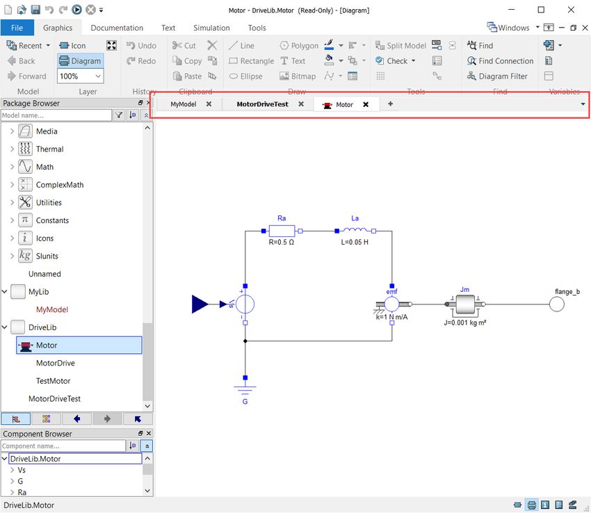
The information in this document is subject to change without notice.

Document version: 1

© Copyright 1992-2020 by Dassault Systèmes AB. All rights reserved.
Dymola® is a registered trademark of Dassault Systèmes AB.
Modelica® is a registered trademark of the Modelica Association.

Other product or brand names are trademarks or registered trademarks of their respective holders.

Dassault Systèmes AB
Ideon Gateway
Scheelevägen 27 – Floor 9
SE-223 63 Lund
Sweden

Support:         http://www.3ds.com/support
URL:             http://www.Dymola.com
Phone:           +46 46 270 67 00
Contents

1      Important notes on Dymola .................................................................................................... 5
2      About this booklet ................................................................................................................... 5
3      Dymola 2021 ............................................................................................................................. 6
    3.1 Introduction ...................................................................................................................................................... 6
       3.1.1   Additions and improvements in Dymola ................................................................................................ 6
       3.1.2   New and updated libraries ...................................................................................................................... 6
    3.2 Developing a model ......................................................................................................................................... 8
       3.2.1   Displaying connector names in the diagram ........................................................................................... 8
       3.2.2   Checking conversion scripts ................................................................................................................... 9
       3.2.3   Minor improvements ............................................................................................................................ 11
    3.3 Simulating a model ........................................................................................................................................ 13
       3.3.1   Analyzing numeric integration ............................................................................................................. 13
       3.3.2   Even logging user interface .................................................................................................................. 14
       3.3.3   Plot tab .................................................................................................................................................. 16
       3.3.4   Animation tab ....................................................................................................................................... 29
       3.3.5   Scripting ............................................................................................................................................... 30
       3.3.6   Saving periodic snapshots during simulation ....................................................................................... 32
       3.3.7   Profiling of function calls ..................................................................................................................... 34
       3.3.8   Minor improvements ............................................................................................................................ 35
    3.4 Installation ...................................................................................................................................................... 40
       3.4.1   Installation on Windows ....................................................................................................................... 40
       3.4.2   Installation on Linux ............................................................................................................................. 42
       3.4.3   Dymola license server on Windows and Linux .................................................................................... 43
    3.5 Model Experimentation .................................................................................................................................. 44
       3.5.1   Scatter plots support in the Design package ......................................................................................... 44
       3.5.2   Minor improvements ............................................................................................................................ 47
    3.6 Other Simulation Environments ..................................................................................................................... 49
       3.6.1   Dymola – Matlab interface ................................................................................................................... 49
       3.6.2   Real-time simulation............................................................................................................................. 49
       3.6.3   Java, Python, and JavaScript Interface for Dymola .............................................................................. 50
       3.6.4   FMI Support in Dymola ....................................................................................................................... 50
    3.7 Modelica Standard Library and Modelica Language Specification ............................................................... 52
    3.8 Documentation ............................................................................................................................................... 52
    3.9 Appendix – Installation: Hardware and Software Requirements ................................................................... 54

                                                                                Dymola 2021 Release Notes                                                                  3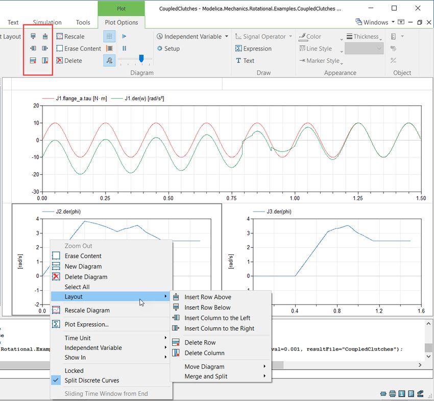
3.9.1   Hardware requirements/recommendations ........................................................................................... 54
    3.9.2   Software requirements .......................................................................................................................... 54

4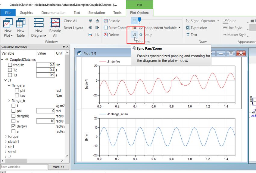
1   Important notes on Dymola
       Installation on Windows
       To translate models on Windows, you must also install a supported compiler. The compiler is
       not distributed with Dymola. Note that administrator privileges are required for installation.
       Three types of compilers are supported on Windows in Dymola 2021:

       Microsoft Visual Studio C++
       This is the recommended compiler for professional users. Both free and full compiler versions
       are supported. Refer to section “Compilers” on page 54 for more information. Note that from
       Dymola 2020x, Visual Studio C++ compilers older than version 2012 are no longer supported.

       Intel
       Dymola 2021 has limited support for the Intel Parallel Studio XE compiler. For more
       information about this compiler, see section “Compilers” on page 54; the section about Intel
       compilers.

       GCC
       Dymola 2021 has limited support for the MinGW GCC compiler, 32-bit and 64-bit. For more
       information about GCC, see section “Compilers” on page 54; the section about GCC
       compilers.

       Installation on Linux
       To translate models, Linux relies on a GCC compiler, which is usually part of the Linux
       distribution. Refer to section “Supported Linux versions and compilers” on page 57 for more
       information.

2   About this booklet
       This booklet covers Dymola 2021. The disposition is similar to the one in Dymola User
       Manuals; the same main headings are being used (except for, e.g., Libraries and
       Documentation).

                                    Dymola 2021 Release Notes                                     5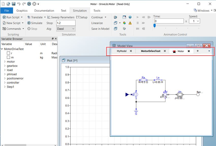
3     Dymola 2021
          Note! From this version of Dymola, Microsoft Windows 7 is not officially supported.

3.1    Introduction
          3.1.1 Additions and improvements in Dymola
          A number of improvements and additions have been implemented in Dymola 2021. In
          particular, Dymola 2021 provides:
            • Option to display connector names in the diagram (page 8)
            • Saving periodic snapshots during simulation (page 32)
            • Improvements to simulation analysis:
                         o Numeric integration: Plotting the scaled local error estimate from the
                              integrator (page 13)
                         o Event log: Filtering of efficient minor events (page 15)
            • GUI for sweeping more than two parameters (page 45)
            • Improvements of plotting:
                         o Support of 2D layout of plot windows (page 16)
                         o New signal operator: Moving Average (page 19)
                         o Scatter plots (page 24)
                         o Plotting Boolean and Integer signals overlapping Real signals (page 21)
                         o Option to synchronize horizontal panning/scrolling for all diagrams in a
                              plot window (page 25)
                         o Adding title and documentation to plot windows (page 23)
            • Profiling function calls (page 34)
            • Checking of conversion scripts (page 9)
            • Using a custom setup file (page 41)
            • License server test when setup (page 43)
            • FMI support improvements
                         o Refresh of FMUs (page 50)

          3.1.2 New and updated libraries
          New libraries
          There are no new libraries in this Dymola version.

6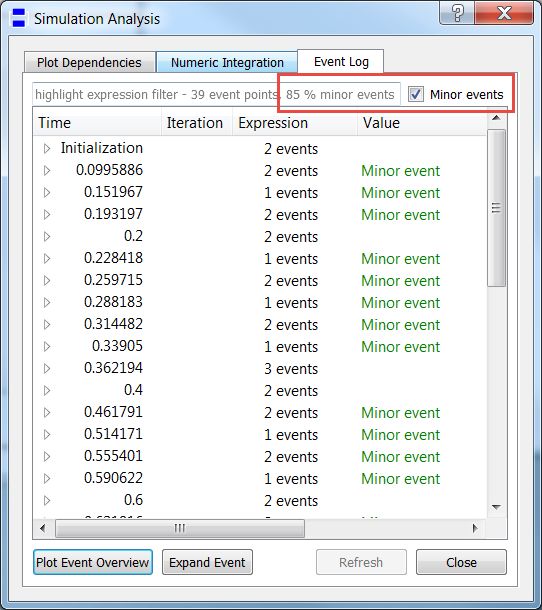
Updated libraries
The following libraries have been updated:
 • Battery Library, version 2.1.4
 • Brushless DC Drives Library, version 1.1.1
 • ClaRa DCS Library, version 1.3.0
 • ClaRa Grid Library, version 1.3.0
 • ClaRa Plus Library, version 1.3.0
 • Claytex Library, version 2019.2
 • Claytex Fluid Library, version 2020.1
 • Cooling Library, version 1.4
 • Dassault Systemes Library, version 1.4
 • Dymola Commands Library, version 1.9
 • Dymola Models Library, version 1.1
 • Electric Power Systems Library, version 1.3.1
 • Electrified Powertrains Library (ETPL), version 1.3.2
 • Fluid Dynamics Library, version 2.9.0
 • Fluid Power Library, version 2020.1
 • FTire Interface Library, version 1.0.4
 • Human Comfort Library, version 2.9.0
 • HVAC (Heating, Ventilation, and Air Conditioning) Library, version 2.9.0
 • Hydrogen Library, version 1.3.2
 • Modelica_DeviceDrivers, version 1.8.2
 • Pneumatic Systems Library, version 1.4
 • Testing Library, version 1.3
 • Thermal Systems Library, version 1.6.0
 • Thermal Systems Mobile AC Library, version 1.6.0
 • VeSyMA (Vehicle Systems Modeling and Analysis) Library, version 2019.2
 • VeSyMA - Engines Library, version 2020.1
 • VeSyMA - Powertrain Library, version 2020.1
 • VeSyMA - Suspensions Library, version 2020.1
 • VeSyMA2ETPL Library, version 2020.1
 • Visa2Base, version 1.8
 • Visa2Paper, version 1.8
 • Visa2Steam, version 1.8
For more information about the updated libraries, please see the Release Notes section in the
documentation for each library, respectively.

                             Dymola 2021 Release Notes                                    7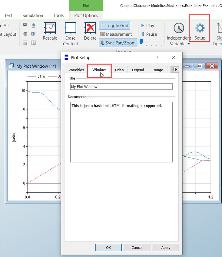
3.2   Developing a model
         3.2.1 Displaying connector names in the diagram
         By the new command Graphics > Connector Names you can display the connector names
         in the diagram. The command works in toggle mode. By default, connector names are not
         shown.

         A corresponding flag Advanced.Editor.ConnectorNameDisplay is available. The flag
         is by default false.

8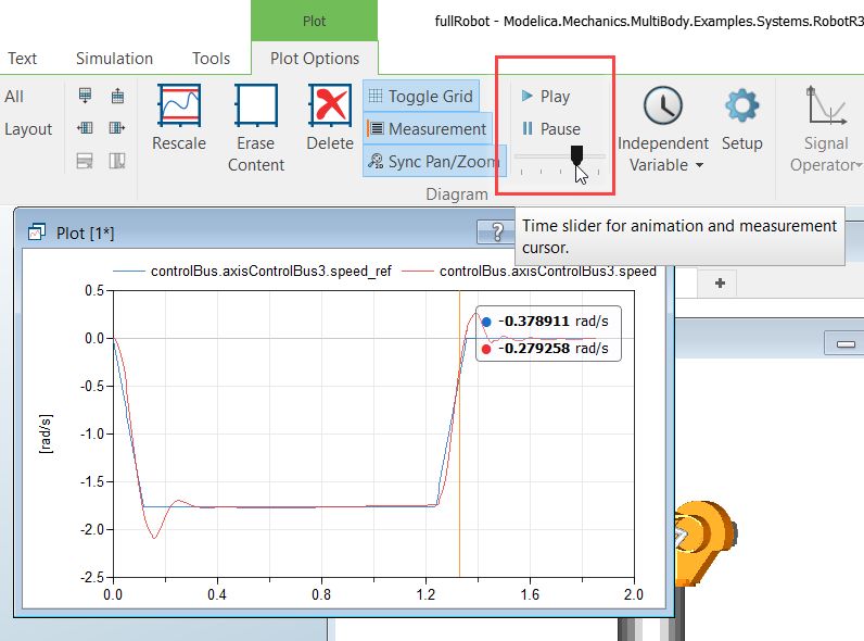
Note that array components/connectors are shown with empty brackets by default. By setting
the flag
       Advanced.ArraySizeInName = true
the array size is also displayed in the brackets (compare the images below).

This flag is by default false.

3.2.2 Checking conversion scripts
A new command button Check is available in the Version tab of the Attributes dialog. This
dialog can be reached by Graphics > Attributes or Text > Attributes:

                             Dymola 2021 Release Notes                                 9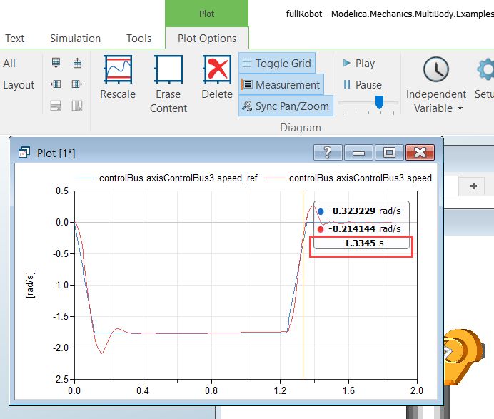
Selecting the conversion script and clicking Check opens a browser for selecting the package
to convert from. When this package is selected, a check of the conversion script is performed,
and the result is displayed.
If the old library is converted to additional libraries you should ideally open them before
checking the conversion, e.g. Modelica normally converts some parts to the
ObsoleteModelica library.
When prompted for the old library you will first be prompted for the old library (including
the version number). If other libraries were merged into the library, you will also be prompted
for them (without version number).
Selecting these libraries are optional.
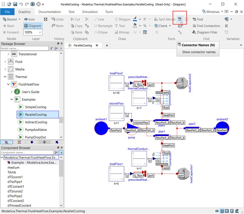
103.2.3 Minor improvements
The Model tabs moved to top of Edit window
The Model tabs are now moved to the top of the Edit window:
This change is valid for all tabs and selections where the model tabs are displayed in the Edit
window.
Dymola 2021 Release Notes 11Indication what flags are stored between sessions
The dialog for setting of flags, reached by Tools > Options > Flags…, now also indicates, by
name in bold, what flags are stored between sessions:
(The dialog above also contains clicking on the “?” and displaying “What´s This” for the
dialog.)
Improved display unit handling
Dymola supports several display units, which are defined at start-up through setup scripts. To
make it easier to use display units suitable for a given application, the user can now control
which setup scripts are executed by setting a variable in Dymola. For example, to run the two
scripts available in the Dymola distribution:
Advanced.DisplayunitSetupPath="$DYMOLA/insert/displayunit.mos;
$DYMOLA/insert/displayunit_us.mos"
By default, $DYMOLA/insert/displayunit.mos is executed at start-up.
Displaying alternatives using Ctrl+Space available in Edit Text dialog
Previously you could display, for example, signal alternatives by the code completion
command Ctrl+Space in the text boxes of the parameter dialog. However, this was not
possible in the text boxes displayed by the context command Edit Text of such input boxes.
This possibility is now added.
12Improved connectorSizing annotation
The connectorSizing annotation now handles a single connection from parametrically sized
component/connector by propagating the parameter.
Improvement of smart connect
The smart connect feature “Connect to connection” is now independent of the flag
Advanced.SmartConnect. The flag now only controls the two features:
• Automatic connect when subcomponents are on top of each other
• Drop components on connection
Improved drawing of arrow heads
The drawing of arrow heads has been changed to follow the Modelica Specification. This
means that the default arrow head size is 5 drawing units, which is slightly bigger than in
previous releases of Dymola. The drawings of arrows in small icons (e.g. in the package
browser) has also been improved.
Minor reorganization of commands in the Tools section of the Graphics
tab
The commands in the Tools section have been somewhat reorganized:
3.3 Simulating a model
3.3.1 Analyzing numeric integration
Scaled local error estimate from the integrator
When you have given the command Simulation > Simulation Analysis, you can, in the
Numeric Integration tab, click Plot Integrator Step Size. In Dymola 2021 a new diagram is
available in the resulting plot. In the figure below, it is the second diagram. In this diagram,
the blue “Scaled local error (estimate)” plots the error estimate from all successful steps. The
red crosses “Rejected steps” marks error estimates from rejected steps. The red line “Scaled
tolerance” is always constant 1.0 representing the limit for a step to be rejected. The integrator
computes local error estimates during simulation, these are rescaled using the tolerance
provided by the user. Thus all local error estimates larger than 1.0 result in a failed step,
whereas all smaller results in a successful step.
Dymola 2021 Release Notes 13The error estimate can for example be used to see if the integration step size is being limited
by the error estimate or something else, like frequent restarts due to events.
3.3.2 Even logging user interface
Improved display of minor events in the event log
By default, efficient minor events are displayed in the event log. They were displayed also in
previous versions, but now they are specifically marked as “minor events” which makes them
more visible. Also the percentage of efficient minor events is now presented:
14Filtering of minor events in the event log
In Dymola 2021, you can deselect Minor events to display only the non-minor events in the
list (compare the figure above):
Dymola 2021 Release Notes 153.3.3 Plot tab
Support of 2D layout of plot windows
Creating the 2D layout
2D layout of plot windows is now supported, using the following new commands:
• To insert or delete rows and columns, the plot diagram context command Layout, or
corresponding buttons in the Plot tab (see the next figure below).
• To insert a diagram in an empty space in a plot window, the context command (for the
empty space) New Diagram.
• To merge diagrams in a plot window, the plot diagram context subcommand Layout >
Merge and Split (see the second next figure below).
• To move a diagram in a 2D plot layout window, two more commands in the new
diagram context subcommand Layout > Move Diagram (for this command, see section
“Additional commands for moving diagrams in a plot window” on page 39).
16The above 2D layout was achieved by, from a plot window with one diagram:
• Right-clicking and selecting Layout > Insert Column to the Right
• Right-clicking the diagram to the right and selecting Layout > Insert Row Below
• Right-clicking the upper left diagram and selecting Layout > Merge and Split > Merge
with Cell to the Right
Notes about merging cells:
• There is no scripting support for merging cells.
Dymola 2021 Release Notes 17• Merging of cells only merges the cells, not the content. The base cell takes over the
space and deletes the overtaken diagram. Illustrating the last command by displaying it
for the left diagram in the second row gives:
For scripting, see section “Scripting support for 2D layout of plot windows” on page 31.
Setting header titles in 2D layout plot windows
You can set headers in 2D layout plot windows using the built-in function
plotRowColumnLabels. As an example, applying, to the example above, the function call
(by, for example, typing it in the command input line of the command window and pressing
return)
plotRowColumnLabels({"Column1", "Column2"}, {"Row1", "Row2"})
the result will be:
18For details about the built-in function plotRowColumnLabels, see “Scripting support for
2D layout of plot windows” on page 31.
New signal operator: Moving Average
A new signal operator Moving Average is available from the context menu of a curve:
Dymola 2021 Release Notes 19Selecting this signal operator as in the figure above, you get: 20
You can specify the horizontal range as well as the interval length. Note that you can also
compute first-order derivatives by activating Differentiate signal in the dialog.
In general, the signal operator is implemented as Centered Moving Average. If any endpoint
is missing for the calculation, it is calculated by interpolation.
The signal operator is also implemented as a built-in function. See “Scripting support for the
signal operator Moving Average” on page 31.

Option to plot Boolean and Integer signals overlapping
In previous Dymola versions, Boolean and Integer signals were only possible to plot using a
special pretty-plotting mode. Now it is possible to display them overlapping by using the plot
diagram context command Split Discrete Curves:

By default, this setting is activated, meaning that the previous behavior of handling the
plotting of the Boolean and Integer signals separately is kept. By deactivating this setting,
Boolean and Integer signals are plotted overlapping in the diagram.
Example with this setting activated (first plot below) and this setting deactivated:

                              Dymola 2021 Release Notes                                   21
The setting corresponds to the flag Advanced.Plot.SplitDiscreteCurves. The flag is
by default true.
The setting/flag is persisted between sessions.
22Adding titles and documentation to plot windows
It is possible to add titles (text in the title bar), and documentation, to plot windows.
To add title and documentation to the active plot window, use the command Plot > Setup,
and select the new Window tab:
Now you can add a window title and documentation, as in the example above. Note that
HTML formatting is supported for the documentation.
Dymola 2021 Release Notes 23The plot window title is seen immediately after clicking OK, as in the plot window title in the
figure above.
To see the plot window documentation, click the question mark in the header of the plot
window. You will get the following:
Note the Edit button, clicking this will open the Window tab of the plot setup, as in the first
figure in this section.
The window title and documentation features are also supported by scripting, see “Adding
titles and documentation to plot windows by scripting” on page 31.
Scatter plots
You can create scatter plots using the new built-in function plotScatter. As an example,
the function call
plotScatter(x={1,2,3}, y={4,5,6}, colors={{0,0,255}, {0,255,0},
{255,0,0}}, markers={MarkerStyle.Cross,
MarkerStyle.FilledSquare, MarkerStyle.Circle})
will result in the plot:
24For details about the built-in function plotScatter, see “Scripting support for scatter plots”
on page 32.
Note that the feature scatter plots is now also available in the Design package, when sweeping
more than two parameters, and also for Monte Carlo Analysis. See “Scatter plots support in
the Design package” starting on page 44.
Option to synchronize horizontal panning and zooming for the diagrams in
a plot window
In previous versions, horizontal zooming was always synchronized for all diagrams in a plot
window.
In Dymola 2021, you can also have synchronized horizontal panning/scrolling.
Both are controlled by the new command button Sync Pan/Zoom in the Plot tab:
Dymola 2021 Release Notes 25The command works in toggle mode. By default, the feature is activated; that is, you have
synchronized panning/scrolling and zooming for all diagrams in the currently active plot
window.
The command is individual for each plot window.
The command button controls the following commands:
• Horizontal zoom: Shift+Drag (with mouse)
• Zoom to curve: Alt+Drag (with mouse)
• Horizontal panning/scrolling: Shift+Mouse wheel
Improved identification of result files
The tooltip for the legend of plotted signals now includes the timestamp (last modified) of the
result file. This makes it easier to identify signal from different result files if the result files
have the same name:
26Time slider, Play button, and Pause button available in the Plot tab
The time slider, the Play button and the Pause button from the Simulation tab is now also
present in the Plot tab:
Dymola 2021 Release Notes 27Note that the time input field and speed setup is however still only available in the Simulation
tab.
Time available in the measurement cursor
By setting the flag
Advanced.Plot.MeasurementTime = true
you will see the time directly in the measurement cursor, like:
The flag is by default false. The flag is saved between sessions.
283.3.4 Animation tab
Time slider available in the Animation tab
The time slider from the Simulation tab is now also present in the Animation tab:
Note that the time input field and speed setup is however still only available in the Simulation
tab.
Dymola 2021 Release Notes 293.3.5 Scripting
A command Open Script available in the Organize Commands dialog
The command Simulation > Commands > Organize Commands opens a dialog for working
with the commands stored in the model. Now this dialog contains a new button Open Script
that can be used to open the .mos script of a command stored as a script:
The script is opened in the Script Editor.
Getting the path of a currently executed .mos script
It is possible to get the path of a currently executed .mos script by using the
classDirectory() function.
As an example, adding this function as a line in a script that is located in the folder
E:\Experiment and then running the script will output, in the command log:
Note that you need to have the option Echo Commands activated to get this output. (The
option is available in the Script Editor tab, in the Options group.)
30Scripting support for 2D layout of plot windows
The built-in function createPlot has been extended to handle subplots. Essentially, the
interpretation of the parameter subPlot in the function has been updated. Note that merging
of cells are not supported by scripting.
To add header titles in 2D layout plot windows, you can use the new built-in function
plotRowColumnLabels:
function plotRowColumnLabels "Set column and row labels in plot window"
input String x[:] = fill("", 0) "Column labels";
input String y[:] = fill("", 0) "Row labels";
input Integer id = 0 "Identity of window (0-means last)";
output Boolean result "true if successful";
external "builtin";
end plotRowColumnLabels;
By default, the header titles are blank. Any unspecified title is blank.
Calling the function with empty titles removes the titles.
For an example, see “Setting header titles in 2D layout plot windows” on page 18.
Adding titles and documentation to plot windows by scripting
It is possible to add titles (text in the title bar) and documentation to plot windows by scripting.
To add a title, use the built-in function plotTitle(title="", id=0). Setting title to an
empty string removes the title, if any.
To add documentation, use the built-in function plotDocumentation(doc="", id=0).
Setting doc to an empty string removes the documentation, if any. HTML formatting is
supported.
These features are also available in the GUI, for more about this, and an example, see “Adding
titles and documentation to plot windows” on page 23.
Scripting support for the signal operator Moving Average
The signal operator Moving Average can be implemented by the built-in function
plotMovingAverage. The function plots a moving average of a plot window.
function plotMovingAverage "Plot moving average in the active diagram of a plot window"
input String variablePath "Variable path or legend name.";
input Real startTime "Start time. In seconds, or base unit if independent variable.";
input Real stopTime "Stop time. In seconds, or base unit if independent variable.";
input Real intervalLength "Averaging interval length";
input Integer order = 0 "Taylor series component (only 0 and 1 are currently
supported)";
input Integer id = 0 "Identity of window (0-means last)";
external "builtin";
end plotMovingAverage;
The function is available in the DymolaCommands library, in the Plot folder.
Dymola 2021 Release Notes 31For more information about this signal operator, see “New signal operator: Moving Average”
on page 19.
Scripting support for scatter plots
To create scatter plots, you can use the new built-in function plotScatter:
function plotScatter "Scatter plot"
input Real x[:] "X-values";
input Real y[size(x, 1)] "Y-values";
input Integer colors[size(x, 1), 3] = fill({-1, -1, -1}, size(x, 1)) "Line colors";
input MarkerStyle markers[size(x, 1)] = fill(MarkerStyle.FilledCircle, size(x, 1))
"Line markers, e.g., MarkerStyle.Cross";
input String legend = "" "Legend describing plotted data";
input Integer axis = 1 "Vertical axis, 1=left, 2=right";
input String unit = "" "Unit";
input Boolean erase = true "Erase window content before plotting";
input Integer id = 0 "Identity of window (0-means last)";
output Boolean result "true if successful";
external "builtin";
end plotScatter;
Each point in the array can have its own color and/or marker style. The default color is the
next available one in the subplot. In an empty subplot the default color is blue. The default
marker style is a filled circle.
The function is available in the DymolaCommands library, in the Plot folder.
For an example, and more applications of scatter plots, see “Scatter plots” on page 24.
New built-in function getLastResultFileName
A new built-in function getLastResultFileName has been added. The function returns a
string with the file name of the last generated simulation result.
The function is available in the DymolaCommands library, in the Trajectories folder.
New built-in function calculateNumberPrecision
A new built-in function calculateNumberPrecision calculates the number of decimals
needed to accurately represent the numbers, from any array of numbers. The result is the
Integer output presision. The function can be used, for example, to adapt result file names
to small parameter values to be able to differ the result files when for example plotting very
small swept parameter values.
The function is available in the DymolaCommands library, in the Plot folder.
3.3.6 Saving periodic snapshots during simulation
To improve the possibility to restart a lengthy simulation from multiple time points, periodic
snapshots can be saved during simulation. The reasons for such restarts could be some
problems in the simulation that needs debugging, or external needs such as restart after each
subtask in a training session.
32The GUI for the option is available in the simulation setup, reached by the command
Simulation > Setup, the Output tab:
The simulator can be instructed to print the simulation result file “dsfinal.txt” snapshots during
simulation. The time interval between such snapshots is controlled by Interval between
snapshots. The default value is 0.0, which means no snapshots. (This setting is also available
as the flag Advanced.Simulation.ResultSnapshotInterval.)
The generated result snapshots can then be used in combination with the command
Simulation > Continue > Import Initial… (or the function importInitial) to continue from
the time of the chosen snapshot. For example, to perform parameter studies from that point.
It is also possible to trigger the generation of snapshots at events. Calling the built-in function
Dymola.Simulation.TriggerResultSnapshot() at an event triggers the creation of a
result snapshot after the event is fully resolved. Example:
Dymola 2021 Release Notes 33when x > 0 then
Dymola.Simulation.TriggerResultSnapshot();
end when;
By default, a time stamp is added to the snapshot file name, e.g.: “dsfinal_0.1.txt”. To turn
off these time stamps, deactivate the setting Time stamps in snapshot file names. This
corresponds to setting the flag
Advanced.Simulation.ResultSnapshotTimeInFileName =false.
A message will be printed in the simulation log whenever a snapshot is created, for example:
... "dsfinal_0.4.txt" creating (snapshot at time t = 0.4)
The settings/flags are persisted between sessions.
3.3.7 Profiling of function calls
It is possible to activate profiling of function calls. This can be used to, for example,
investigate external function calls, especially FMUs. Another usage can be to find time-
consuming media functions.
To activate profiling of function calls, set the flag
Advanced.GenerateFunctionTimers = true
(The flag is by default false.)
This profiling can be used together with the profiling available in previous versions, activated
by
Advanced.GenerateBlockTimers = true
The new profiling of functions can also be used on its own.
Note however that any profiling demands the flag
Advanced.Define.PrecisionTiming = true
343.3.8 Minor improvements
Model tabs in Model View window
Model tabs are now also present in the Model View window:
Improved identification of result files in the variable browser
The tooltip for the result (file) in the variable browser now includes the timestamp (last
modified) of the result file. This makes it easier to identify signals from different result files
if the result files have the same name.
Dymola 2021 Release Notes 35Variable frequency of output points
Normally the interval length (or indirectly the number of output points) determines the
frequency of results.
By setting the flag:
Advanced.Simulation.VariableInterval=true;
And in the model use
when time>=… then
Dymola.Simulation.SetOutputInterval(…);
end when;
the frequency can be controlled from the model.
Note that the simulation setup is used until the first call of
Dymola.Simulation.SetOutputInterval(…);
A full example, with stop time set to 2 and interval length set to 0,002 in the simulation setup,
and then running:
model VariableOutputInterval
"demonstrate the use of variable output interval in a model"
Real x;
equation
x = sin(10*time);
when initial() then
Dymola.Simulation.SetOutputInterval(0.1);
end when;
when time >= 0.5 then
Dymola.Simulation.SetOutputInterval(0.05);
end when;
when time >= 1.1 then
Dymola.Simulation.SetOutputInterval(0.002);
end when;
end VariableOutputInterval;
will give the below curve when plotted:
36Notes:
• The only way to “reset” the interval length to the one in the simulation setup is to
explicitly set that interval, this is done in the last when statement above.
• You must have a separate when statement for each time.
Option to save plot window setup as a command based on the proposed
Modelica standard
You can save the plot window setup based on the proposed Modelica standard for pre-defined
plots by activating the setting Based on proposed Modelica standard in the dialog for
saving a command to the model.
Dymola 2021 Release Notes 37You can get the dialog above by the command Simulation > Commands > Add Command….
Option to let the Simulate button in the quick access toolbar switch to
Simulation tab
By using the flag Advanced.Simulation.SwitchToSimulation you can decide if using
the Simulate button in the quick access toolbar should also switch to displaying the
Simulation tab.
By default, the flag is false, meaning there is no switching of display to the Simulation tab.
Analyzing Numeric Integration: Showing the component from the context
menu of a variable in the Numeric Integration tab
In the previous version of Dymola, you could, in the Event Log tab of the Simulation
Analysis window, right-click a variable and select Show Component to show either the
corresponding component highlighted in the diagram, or show the corresponding variable
highlighted (search hits) in the Modelica Text code.
This context menu entry is now also available for the variables in the Numeric Integration
tab of the Simulation Analysis window:
38The command Analyze Numerics is renamed to Simulation Analysis
The command Simulation > Analyze Numerics is now renamed to Simulation > Simulation
Analysis to be more consistent with the content and the title of the corresponding dialog.
Rearrangement of the Output tab of the simulation setup
In the Output tab of the simulation setup, the Store additional variables group has been
moved, to enable the addition of the Complete result snapshots group. Please see the image
in section “Saving periodic snapshots during simulation” on page 32 for the new location.
Additional commands for moving diagrams in a plot window
Because of the new option to have 2D layout of plot windows, two new commands for moving
a diagram in a plot window have been added. The commands have also been grouped to a
new subcommand entry Layout > Move Diagram in the plot diagram context command:
Dymola 2021 Release Notes 39The two new commands are framed in the image above.
Improved handling of nonlinear model equations
Improvements have been made to Dymola’s solver of nonlinear model equations. The solver
is now more reliable, accurate, and efficient. Models with large and nonlinear algebraic loops
may simulate faster. Similarly, inline simulations using implicit methods may run faster.
3.4 Installation
For the current list of hardware and software requirements, please see chapter “Appendix –
Installation: Hardware and Software Requirements” starting on page 54.
3.4.1 Installation on Windows
For the full list of supported compilers, see “Compilers” on page 54.
Discontinued support for Windows 7
This version of Dymola does not officially support Microsoft Windows 7 operating system.
40Option to use a custom setup file
In Dymola 2021 it is possible run Dymola with a custom setup file. This enables having setups
for different project; for example:
• Preloading project-specific libraries
• Maintaining conflicting and alternative library versions by having different Modelica
paths
• Setups tailored for simulation, customer-specific presentations, or with GUI layout
optimized for projectors
• Using different compiler settings for different customers
You can in fact copy the whole Dymola installation to another location, and use a custom
setup file when starting the copy, using the command line as below. This copy of Dymola will
be totally independent from the original, except for the licensing.
To specify the path to the custom setup.dymx file, the command line argument –setup is
used; for example
Dymola.exe –setup "E:\MyExperiments\MyCustom1Setup.dymx"
If this file cannot be found, an error message appears:
You have the following alternatives:
• Create File tries to create an empty setup.dymx at the specified location.
• Use Default uses the default setup file, on Windows typically:
C:\Users\\AppData\Roaming\DassaultSystemes\Dymola\2021\
setup.dymx
• Exit Dymola exits Dymola. if Dymola is started with any of the command line
arguments –nowindow or –externalinterface then Dymola is exited with an error
code.
Option to not save any changes in the setup file
There is a new command line argument –nosavesettings in Dymola 2021 that loads the
setup file but does not save it. Any changes that you do in Dymola will thus not be changed
in the settings file.
Note the command line argument –nosettings that specifies that the setup should not be
loaded or saved. This argument has existed since a few versions.
Dymola 2021 Release Notes 41Updated Qt version
Dymola 2021 is built with Qt 5.14.1.
Microsoft Visual Studio compilers
Extended checking when using Verify Compiler
Using the Verify Compiler command button now also checks if an unsupported Visual Studio
compiler version has been selected by using the Visual Studio Custom alternative. For
example, specifying the path to a Visual Studio 2010 compiler and clicking Verify Compiler
gives the message:
In the command log the following message is given:
3.4.2 Installation on Linux
GUI for selecting and testing of compiler
You can now use a dialog to select compiler, set linker flags, and test the compiler by the
Verify Compiler button, like in Windows. This is done by the command Simulation > Setup,
in the Compiler tab.
Option to use a custom setup file
The feature is the same as for Windows, see above, except that Linux have other paths; for
example, the default path for the default setup file in Linux is, under the user´s home directory:
42.dassaultsystemes/Dymola/2021/setup.dymx
Option to not save any changes in the setup file
See the corresponding section for Windows above.
Updated Qt version
Dymola 2021 is built with Qt 5.14.1.
3.4.3 Dymola license server on Windows and Linux
Testing the license server at setup
Basic DNS lookup check for server host name
When trying to connect to the license server host; a basic DNS lookup check is performed. If
the host cannot be found, the following message appears:
If the host is found, a ping test is performed, and a test checkout of Dymola Standard license
is requested from this server. An example with successful ping test but failed Dymola license
checkout test:
Dymola 2021 Release Notes 43It is still possible to change the license file by answering Change Server Settings on the
following question whether to update the license server. This can be used for additional
testing.
3.5 Model Experimentation
3.5.1 Scatter plots support in the Design package
New functions
The scatter plots support is included in the Design.Experimentation package, as three new
functions:
44• MonteCarloAnalysisScatter – performs a Monte Carlo analysis and presents the result
as a matrix of color-coded scatter plots.
• sweepManyParametersScatter – sweeps more than two parameters and presents the
result as a matrix of color-coded scatter plots (see example below).
• ScatterPlots (in the Analysis subpackage) – this function is used by the two functions
above, but can also be used to produce color-coded scatter plots from results from other
sources.
Example: GUI for sweeping more than two parameters
Already previous Dymola versions supported sweeping more than two parameters but there
was no support for any corresponding plotting. Now, with the scatter plots functionality, that
support is available. As an example, for the Coupled Clutches demo, with the following
sweeping setup:
Dymola 2021 Release Notes 45you will get the following plot: 46
The problem we want to solve is to understand how variations in many parameters explain
the variation in the output variable, and it’s not simply explained by changes in individual
variables. Thus we take the next step and see whether pairs of variables explain the variation
in the “output” variable.
That explains the non-diagonal entries in the matrix of scatter plots, and that part is symmetric
(the pair J1.J, J2.J behave the same as J2.J, J1.J). The output value is given as the color of the
dots, and since we sweep parameters the scattering of the points does not provide any useful
information. There are two ways of using that information:
   • Select one parameter and see which parameter combines with it to best explain the
      output.
   • See which pair-wise combination overall are the most important.
Using the same logic for the diagonal entries would just be uninteresting straight lines since
it is the same parameter on both axis; and normally a matrix of scatter plots includes
something else.
In this case it is just a color-coded plot of the output variable against the parameter; there are
two ways of using this information:
  • It shows how much variations in that parameter explain the variation in the output
      variable – if the other parameters had no impact it would just be a curved line – and the
      other parameters would turn it into a “fatter” line.
  • As references for the color-scale of the output variables.
General references:
https://www.itl.nist.gov/div898/handbook/eda/section3/eda33qb.htm
https://plot.ly/python/splom/
Note the possibility to use Monte Carlo analysis rather that sweeping when working with
many variables, Monte Carlo is more efficient in such cases. In this Dymola version, as noted
above, Monte Carlo analysis can also be presented by color-coded scatter plots.

3.5.2 Minor improvements
Generating grid with logarithmic scale for sweeping
You can now generate grid with logarithmic scale when setting up sweeping of parameters,
by selecting Logarithmic scale in the dialog for the grid:

                                Dymola 2021 Release Notes                                     47
By default, this option is not activated.
Progress indicator when sweeping parameters
When sweeping parameters, the progress indicated the same way as the simulation in Dymola;
there is a green progress bar in the background of the Dymola icon in the taskbar.
Error message when trying to sweep evaluated parameters
When trying to sweep an evaluated parameter, you will get an error message. As an example,
opening the demo Coupled Clutches, setting Evaluate =true (by typing it on the command
input line of the command window and pressing Enter), and then trying to sweep J1.J and
plotting J1.w, you get the following message:
483.6 Other Simulation Environments
3.6.1 Dymola – Matlab interface
Compatibility
The Dymola – Simulink interface now supports Matlab releases from R2015a (ver. 8.5) up to
R2019b (ver. 9.7). On Windows, only Visual Studio C++ compilers are supported to generate
the DymolaBlock S-function. On Linux, the gcc compiler is supported. The LCC compiler is
not supported, neither on Windows nor Linux.
3.6.2 Real-time simulation
Compatibility – dSPACE
Dymola 2021 officially supports the DS1005, DS1006, MicroLabBox, and SCALEXIO
systems for HIL applications. For these systems, Dymola 2021 generated code has been
verified for compatibility with the following combinations of dSPACE and Matlab releases:
• dSPACE Release 2015-A with Matlab R2015a
• dSPACE Release 2015-B with Matlab R2015b
• dSPACE Release 2016-A with Matlab R2016a
• dSPACE Release 2016-B with Matlab R2016b
• dSPACE Release 2017-A with Matlab R2017a
• dSPACE Release 2017-B with Matlab R2017b
• dSPACE Release 2018-A with Matlab R2018a
• dSPACE Release 2018-B with Matlab R2018b
• dSPACE Release 2019-A with Matlab R2018b and R2019a
• dSPACE Release 2019-B with Matlab R2018b, R2019a, and R2019b
The selection of supported dSPACE releases focuses on releases that introduce support for a
new Matlab release and dSPACE releases that introduce a new version of a cross-compiler
tool. In addition, Dymola always support the three latest dSPACE releases with the three latest
Matlab releases. Although not officially supported, it is likely that other combinations should
work as well.
New utility functions – dym_rti_build2 and dym_rtimp_build2
Dymola 2021 introduces a new function, dym_rti_build2, that replaces dym_rti_build
for building dSPACE applications from models containing DymolaBlocks. The new function
uses the new dSPACE RTI function rti_build2 instead of the old function rti_build.
A corresponding new multi-processor build function, dym_rtimp_build2, is also
introduced.
These functions are supported with dSPACE Release 2019-B and later.
Dymola 2021 Release Notes 49Note on dym_rti_build and dSPACE Release 2017-A and later
The function rti_usrtrcmerge is no longer available in dSPACE Release 2017-A and later.
As a consequence, it is required to run the standard rti_build function (with the ‘CM’
command) after dym_rti_build to get your _usr.trc content added to the main .trc file. For
example:
>> dym_rti_build('myModel', 'CM')
>> rti_build('myModel', 'Command', 'CM')
Note that this note applies the new functions dym_rti_build2 and rti_build2 as well.
Compatibility – Simulink Real-Time
Compatibility with Simulink Real-Time has been verified for all Matlab releases that are
supported by the Dymola – Simulink interface, which means R2015a (Simulink Real-Time
ver. 6.2) to R2019b (Simulink Real-Time ver. 6.11). Only Microsoft Visual C compilers have
been tested.
3.6.3 Java, Python, and JavaScript Interface for Dymola
A number of new and improved built-in functions are available in the interfaces.
For more information, see the corresponding section in “Scripting” on page 30.
3.6.4 FMI Support in Dymola
Unless otherwise stated, features are available both for FMI version 1.0 and version 2.0.
Profiling of external FMU function calls
Please see section “Profiling of function calls” on page 34.
FMU Import
Refresh of FMUs
FMU components can in Dymola 2021 be refreshed by using the FMU context command Re-
Import FMU:
50There is no scripting support for this functionality.
Check if Windows binaries are available when importing an FMU in Windows
When you import an FMU in Windows that contains no Windows binaries, you will get a
warning.
The warning when importing by the command File > Open > Import FMU… or dragging the
FMU into the Dymola window:
Dymola 2021 Release Notes 51The warning in the Command log when importing the FMU by scripting:
Support for using the step size for imported co-simulation FMUs
If the step size has been set for an exported co-simulation FMU from another vendor, this step
size is used when the FMU is imported to Dymola. The value is displayed in the FMI tab of
the parameter dialog of the instantiated FMU, in the Step time group, the parameter
fmi_CommunicationStepSize.
3.7 Modelica Standard Library and Modelica
Language Specification
The current version of the Modelica Standard Library is version 3.2.3. The current version of
the Modelica Language Specification is 3.4.
Note that the Modelica Standard Library version 3.2.3 is compliant with the Modelica
Language Specification 3.4. (So this version of the Modelica Language Specification should
be used for reference, and not the Modelica Language Specification 3.2, Revision 2.)
3.8 Documentation
General
In the previous version of Dymola, the former Dymola User Manual Volume 1 was split in
two manuals:
• “Dymola User Manual 1A: Introduction, Getting Started, and Installation”, containing
the following chapters:
o What is Dymola?
o Getting started with Dymola
o Introduction to Modelica
o Appendix - Installation
• “Dymola User Manual 1B: Developing and Simulating a Model”, containing the
following chapters:
52o Developing a model
o Simulating a model
In this version of Dymola, the former Dymola User Manual Volume 2 is also split, in three
manuals:
• “Dymola User Manual 2A: Model Development Tools”, containing the following
chapters:
o Model Experimentation
o Model Calibration
o Design Optimization
o Model Management
• “Dymola User Manual 2B: Simulation Interfaces and Export”, containing the following
chapters:
o FMI Support in Dymola
o Simulation Environments
o Scripting and Reporting
• “Dymola User Manual 2C: Advanced Concepts”, containing the following chapters:
o Advanced Modelica Support
o Visualize 3D
o User-defined GUI
o Appendix - Migration
In the software distribution of Dymola 2021 Dymola User Manuals of version “March 2020”
will be present; these manuals include all relevant features/improvements of Dymola 2021
presented in the Release Notes.
Dymola 2021 Release Notes 533.9 Appendix – Installation: Hardware and Software
Requirements
Below the current hardware and software requirements for Dymola 2021 are listed.
3.9.1 Hardware requirements/recommendations
Hardware requirements
• At least 2 GB RAM
• At least 400 MB disc space
Hardware recommendations
At present, it is recommended to have a system with an Intel Core 2 Duo processor or better,
with at least 2 MB of L2 cache. Memory speed and cache size are key parameters to achieve
maximum simulation performance.
A dual processor will be enough if not using multi-core support; the simulation itself, by
default, uses only one execution thread so there is no need for a “quad” processor. If using
multi-core support, you might want to use more processors/cores.
Memory size may be significant for translating big models and plotting large result files, but
the simulation itself does not require so much memory. Recommended memory size is 6 GB
of RAM.
3.9.2 Software requirements
Microsoft Windows
Dymola versions on Windows and Windows operating systems versions
Dymola 2021 is supported, as 64-bit application, on Windows 8.1, and Windows 10. Since
Dymola does not use any features supported only by specific editions of Windows (“Home”,
“Professional”, “Enterprise” etc.), all such editions are supported if the main version is
supported.
Compilers
Please note that for the Windows platform, a Microsoft C/C++ compiler, an Intel compiler,
or a GCC compiler, must be installed separately. The following compilers are supported for
Dymola 2021 on Windows:
Microsoft C/C++ compilers, free editions:
Note. When installing any Visual Studio, make sure that the option “C++/CLI support…” is
also selected to be installed.
• Visual Studio 2012 Express Edition (11.0)
54• Visual Studio 2013 Express Edition for Windows Desktop (12.0)
• Visual Studio 2015 Express Edition for Windows Desktop (14.0)
• Visual Studio 2017 Desktop Express (15) Note! This compiler only supports compiling
to Windows 32-bit executables.
• Visual Studio 2017 Community 2017 (15)
• Visual Studio 2017 Build Tools Notes:
o The recommended selection to run Dymola is the workload “Visual C++
build tools” + the option “C++/CLI Support…”
o Installing this selection, no IDE (Integrated Development Environment)
is installed, only command line features
o This installation is not visible as a specific selection when later selecting
the compiler in Dymola, the alternative to select is the same as for any
Visual Studio 2017 alternative: Visual Studio 2017/Visual C++ 2017
Express Edition (15).
o For more information about installing and testing this compiler with
Dymola, see www.Dymola.com/compiler.
• Visual Studio 2019 Community (16)
• Visual Studio 2019 Build Tools Notes:
o The recommended selection to run Dymola is the workload “C++ build
tools” + the option “C++/CLI Support…”
o Installing this selection, no IDE (Integrated Development Environment)
is installed, only command line features
o This installation is not visible as a specific selection when later selecting
the compiler in Dymola, the alternative to select is the same as for any
Visual Studio 2019 alternative: Visual Studio 2019/Visual C++ 2019
(16).
o For more information about installing and testing this compiler with
Dymola, see www.Dymola.com/compiler.
Microsoft C/C++ compilers, professional editions:
Note. When installing any Visual Studio, make sure that the option “C++/CLI support…” is
also selected to be installed
• Visual Studio 2012 (11.0)
• Visual Studio 2013 (12.0)
• Visual Studio 2015 (14.0)
• Visual Studio Professional 2017 (15)
• Visual Studio Enterprise 2017 (15)
• Visual Studio Professional 2019 (16)
• Visual Studio Enterprise 2019 (16)
Intel compilers
The Intel compilers Intel Parallel Studio XE 2016, XE 2017, and XE 2018 are supported.
Dymola 2021 Release Notes 55Note that you must also select a Visual Studio compiler when selecting any Intel compiler.
Supported combinations of Intel compilers and Visual Studio compilers:
• Intel Parallel Studio XE 2016: Visual Studio 2012, 2013, or 2015
• Intel Parallel Studio XE 2017: Visual Studio 2012, 2013, 2015, or 2017
• Intel Parallel Studio XE 2018: Visual Studio 2013, 2015, or 2017
Current limitations:
• Embedded server (DDE or OPC) is not supported.
• Export DLL is not supported.
GCC compilers
Dymola 2021 has limited support for the MinGW GCC compiler. The following versions
have been tested:
• For 32-bit GCC: version 4.8.1, 5.3, 6.3, and 8.2
• For 64-bit GCC: version 4.9.2, 5.3, 7.3, and 8.1
Hence, at least the versions in that range should work fine.
To download any of these free compilers, please visit http://www.Dymola.com/compiler
where the latest links to downloading the compilers are available. Needed add-ons during
installation etc. are also specified here. Note that you need administrator rights to install the
compiler.
Also note that to be able to use other solvers than Lsodar, Dassl, and Euler, you must also add
support for C++ when installing the GCC compiler. Usually, you can select this as an add-on
when installing GCC.
Current limitations with 32-bit and 64-bit GCC:
• Embedded servers (DDE or OPC servers) are not supported.
• Support for external library resources is implemented, but requires that the resources
support GCC, which is not always the case.
• FMUs must be exported with the code export option 1 enabled.
• For 32-bit simulation, parallelization (multi-core) is currently not supported for any of
the following algorithms: RadauIIa, Esdirk23a, Esdirk34a, Esdirk45a, and Sdirk34hw.
• Compilation may run out of memory also for models that compile with Visual Studio.
The situation is better for 64-bit GCC than for 32-bit GCC.
In general, 64-bit compilation is recommended for MinGW GCC. In addition to the
limitations above, it tends to be more numerically robust.
1
Having the code export options means having any of the license features Dymola Binary Model Export or the
Dymola Source Code Generation.
56You can also read